Cosmological inflation
David Langlois(APC, Paris)
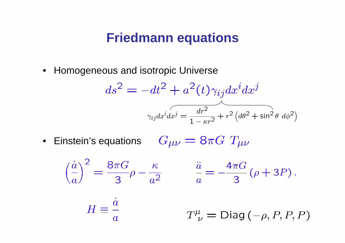
Friedmann equations
• Homogeneous and isotropic Universe
• Einstein’s equations

The Universe in the Past
The energy densities dilute at various rates:– pressureless matter
– radiation
Time
matter-radiation equality
nucleosynthesis
now
last scattering

Cosmic Microwave Background (CMB)
• T> 3.103 K: atoms are ionised (H→ p+e-) ⇒ opaque Universe
• T< 3.103 K: “recombination” (p+e-→ H)⇒ transparent Universe
• “Fossil” background radiation – predicted in 1948,– discovered in 1965 by Penzias and
Wilson.
T≃ 2.7 K

COBE satellite
"for their discovery of the blackbody formand anisotropy of the cosmic microwavebackground radiation"
John C. Mather George F. Smoot
Nobel Prize in Physics 2006
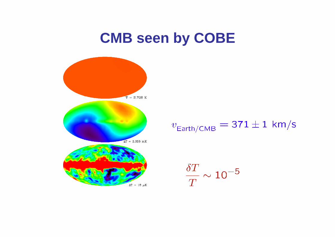
CMB seen by COBE
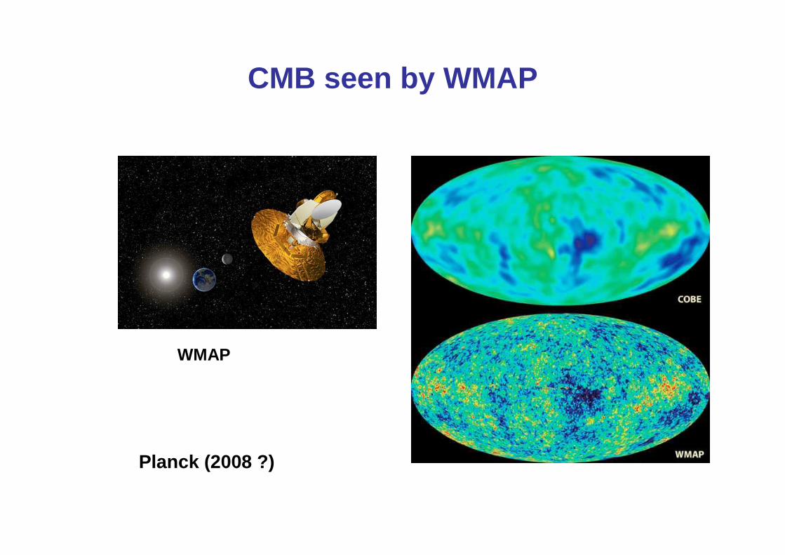
WMAP
Planck (2008 ?)
CMB seen by WMAP
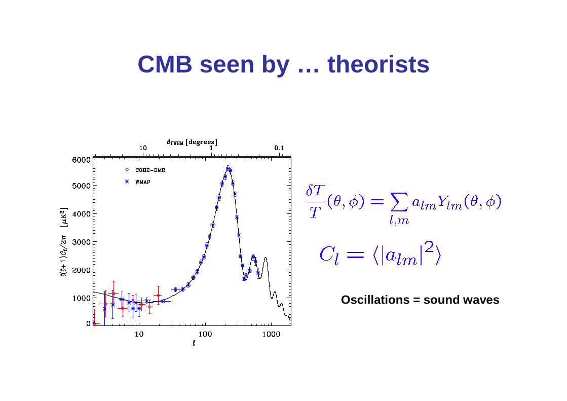
CMB seen by … theorists
Oscillations = sound waves
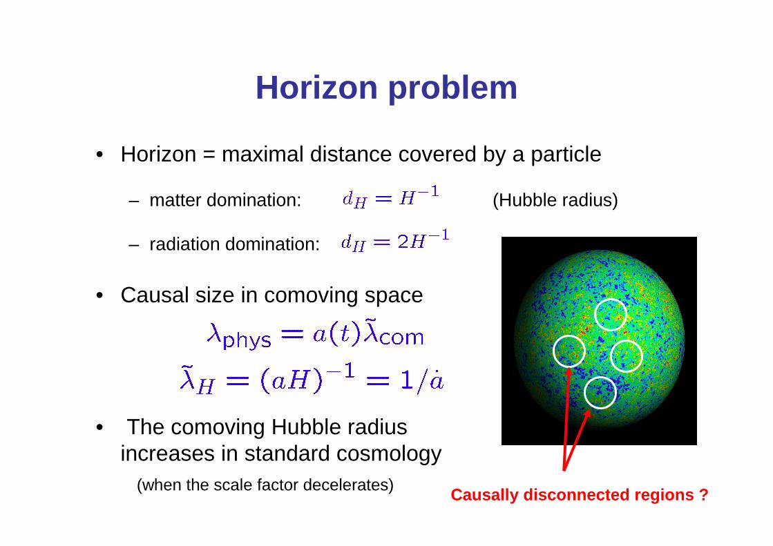
Horizon problem
• Horizon = maximal distance covered by a particle
– matter domination: (Hubble radius)
– radiation domination:
• Causal size in comoving space
• The comoving Hubble radius increases in standard cosmology
(when the scale factor decelerates)Causally disconnected regions ?
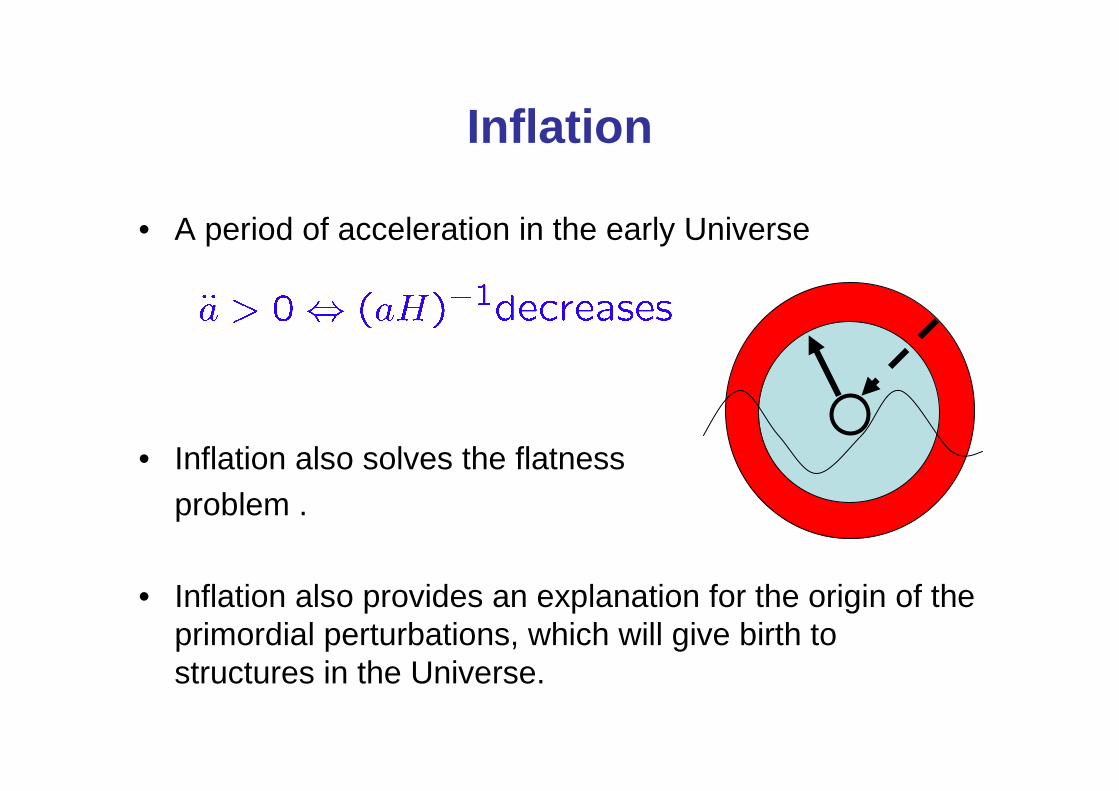
Inflation
• A period of acceleration in the early Universe
• Inflation also solves the flatnessproblem .
• Inflation also provides an explanation for the origin of the primordial perturbations, which will give birth to structures in the Universe.

Scalar field inflation
• How to get inflation ?
• Scalar field
• Homogeneous equations
• Slow-roll motion
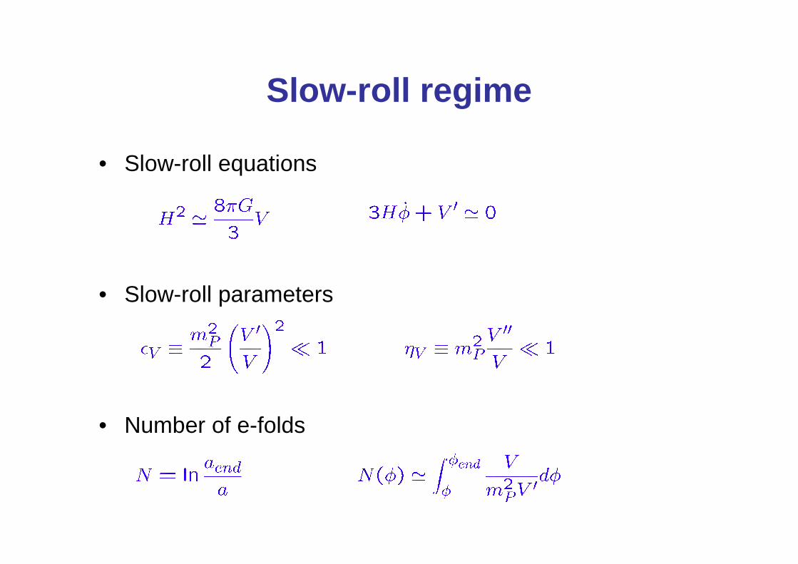
Slow-roll regime
• Slow-roll equations
• Slow-roll parameters
• Number of e-folds

Cosmological perturbations
• Matter: perfect fluid
• Perturbed metric (with only scalar perturbations)
• related to the intrinsic curvature of constant time spatial hypersurfaces
• Change of coordinates, e.g.
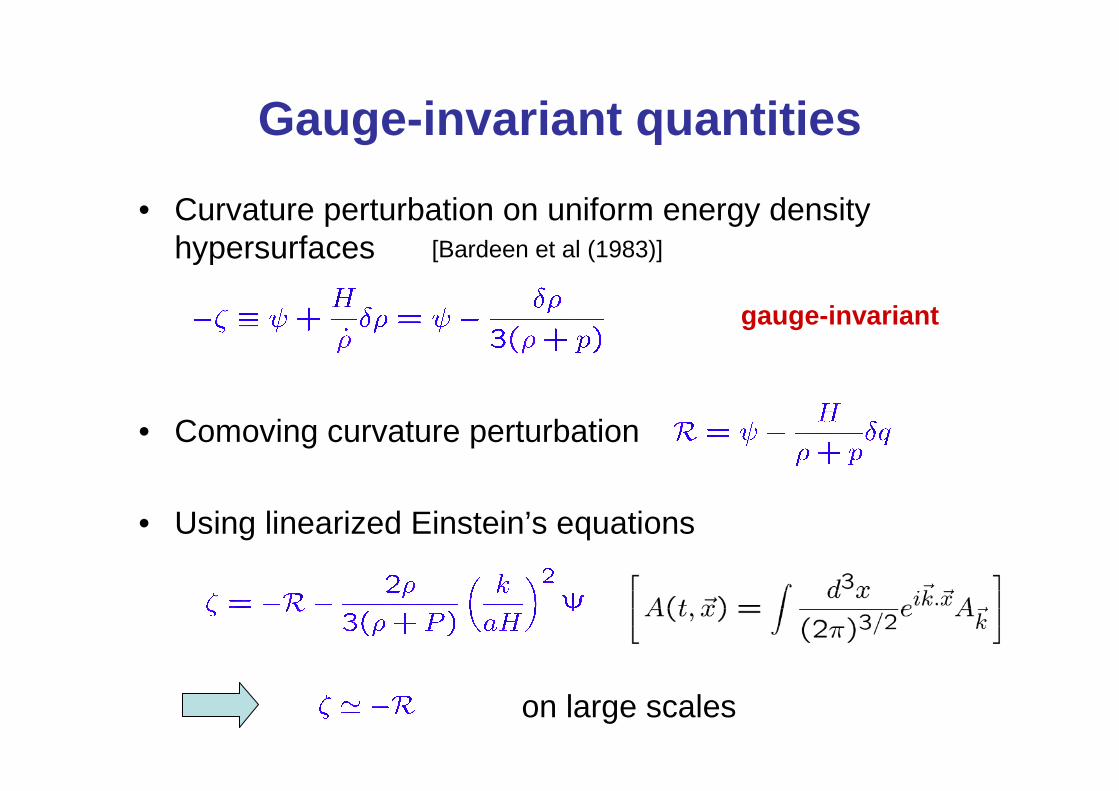
Gauge-invariant quantities
• Curvature perturbation on uniform energy density hypersurfaces
• Comoving curvature perturbation
• Using linearized Einstein’s equations
on large scales
gauge-invariant
[Bardeen et al (1983)]
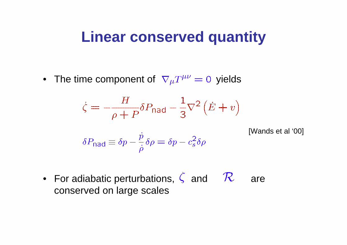
Linear conserved quantity
• The time component of yields
• For adiabatic perturbations, and are conserved on large scales
[Wands et al ‘00]
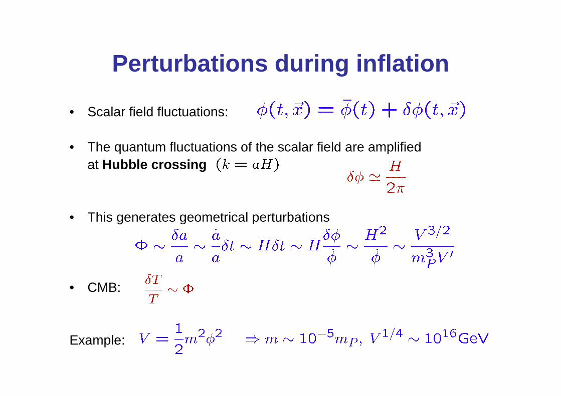
Perturbations during inflation
• Scalar field fluctuations:
• The quantum fluctuations of the scalar field are amplified at Hubble crossing
• This generates geometrical perturbations
• CMB:
Example:

Some details…
• Massless scalar field
using the conformal time
• De Sitter spacetime
• New function
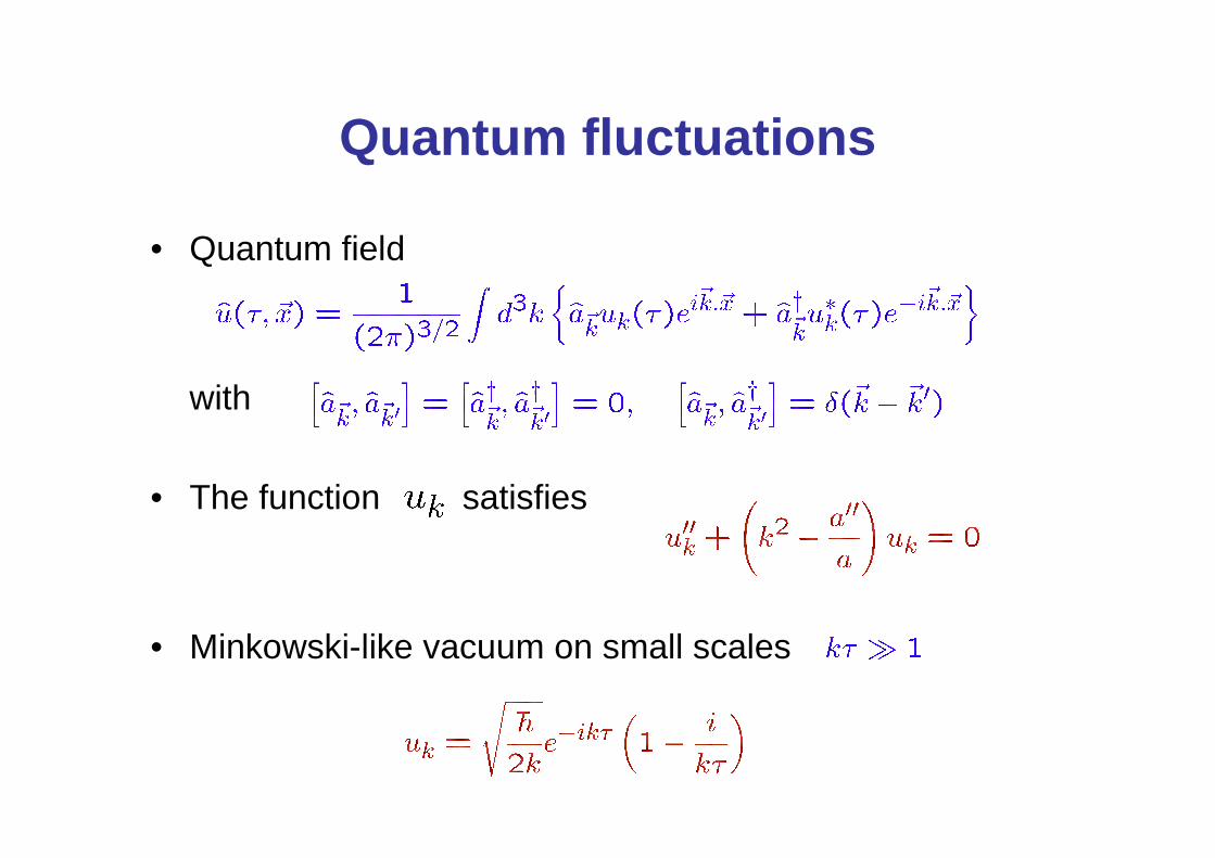
Quantum fluctuations
• Quantum field
with
• The function satisfies
• Minkowski-like vacuum on small scales
Quantum fluctuations
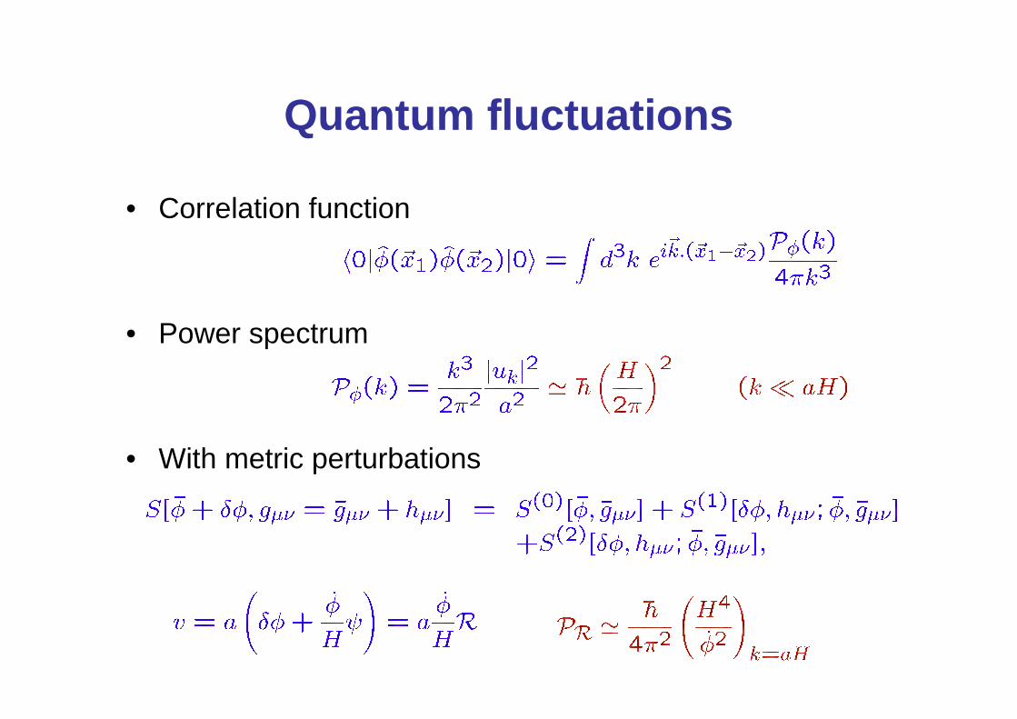
• Correlation function
• Power spectrum
• With metric perturbations
Scalar perturbations from inflation
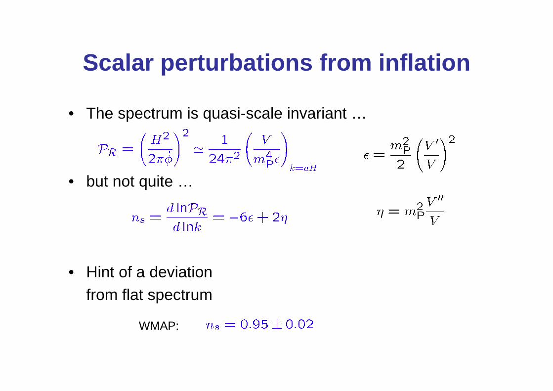
• The spectrum is quasi-scale invariant …
• but not quite …
• Hint of a deviation from flat spectrum
WMAP:
Gravitational waves from inflation
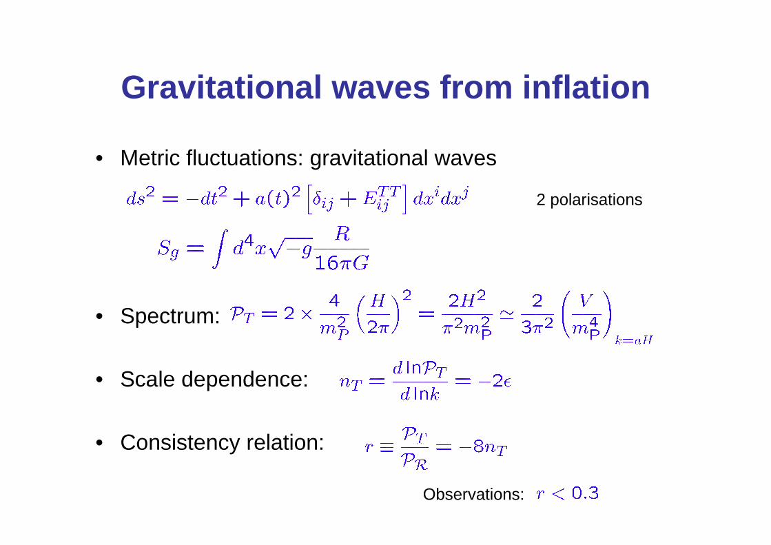
• Metric fluctuations: gravitational waves
• Spectrum:
• Scale dependence:
• Consistency relation:
2 polarisations
Observations:
Multi-field inflation
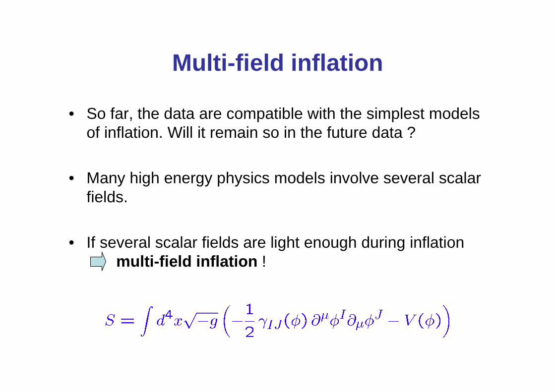
• So far, the data are compatible with the simplest models of inflation. Will it remain so in the future data ?
• Many high energy physics models involve several scalar fields.
• If several scalar fields are light enough during inflation multi-field inflation !
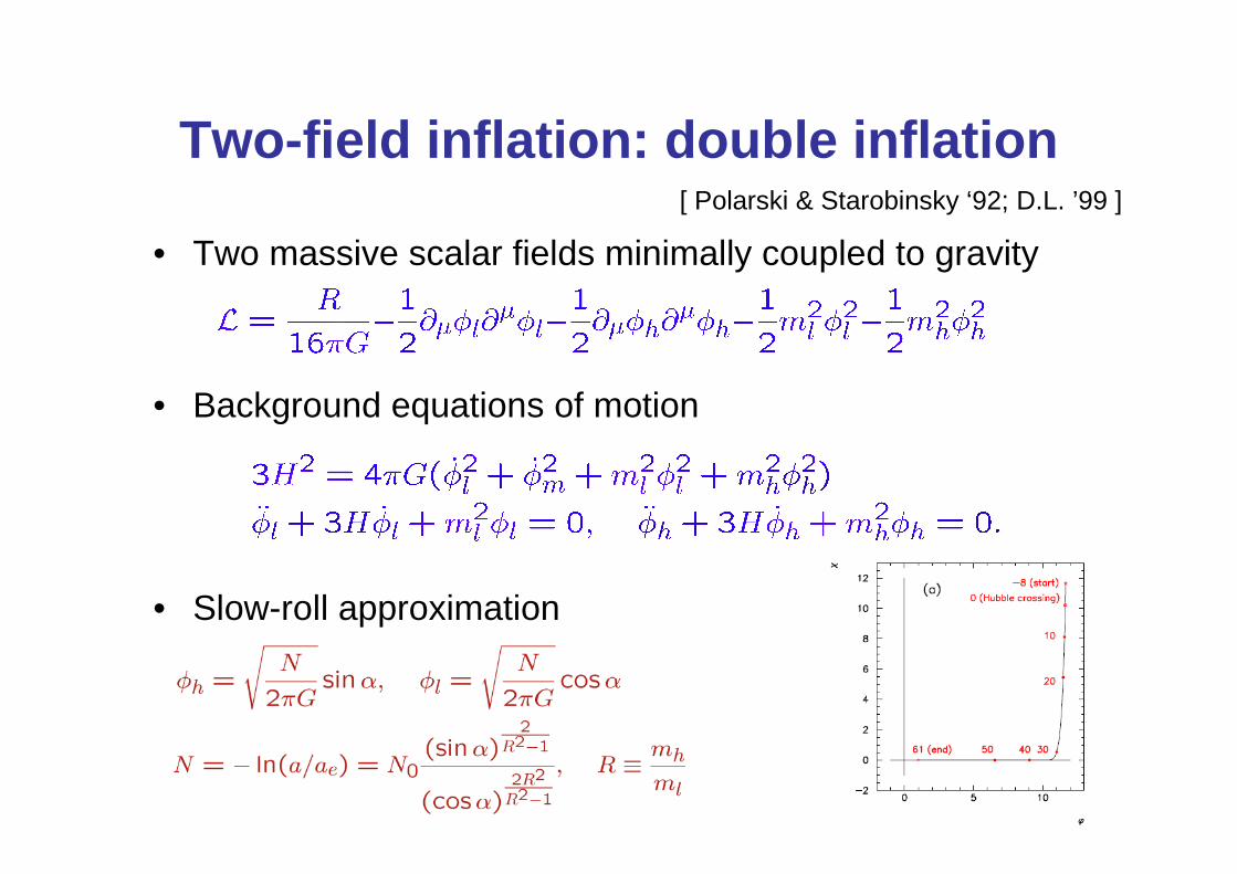
Two-field inflation: double inflation
• Two massive scalar fields minimally coupled to gravity
• Background equations of motion
• Slow-roll approximation
[ Polarski & Starobinsky ‘92; D.L. ’99 ]

Double inflation: perturbation equations
• Metric:
• Linearized Einstein and Klein-Gordon equations yield
• In the slow-roll approximation and for large scales,
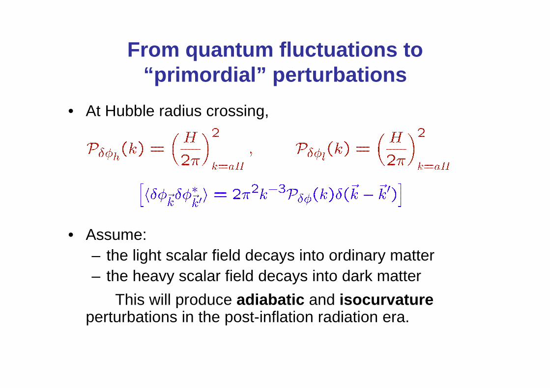
From quantum fluctuations to “primordial” perturbations
• At Hubble radius crossing,
• Assume: – the light scalar field decays into ordinary matter– the heavy scalar field decays into dark matter
This will produce adiabatic and isocurvatureperturbations in the post-inflation radiation era.

Adiabatic and isocurvature perturbations
• In the radiation era:– Adiabatic / curvature perturbations
– Entropy / isocurvature perturbations
• They can be related to the perturbations during inflation:
Correlation between adiabatic and isocurvature perts !
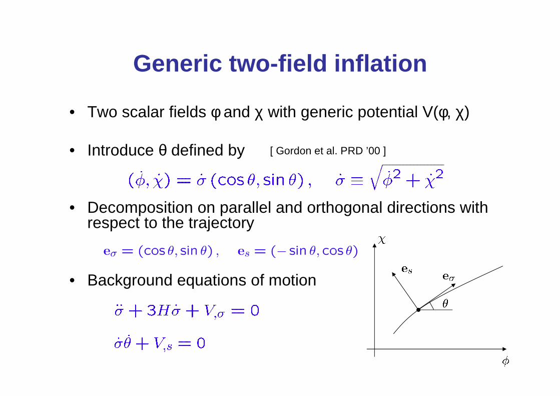
Generic two-field inflation
• Two scalar fields φ and χ with generic potential V(φ, χ)
• Introduce θ defined by
• Decomposition on parallel and orthogonal directions with respect to the trajectory
• Background equations of motion
[ Gordon et al. PRD ’00 ]
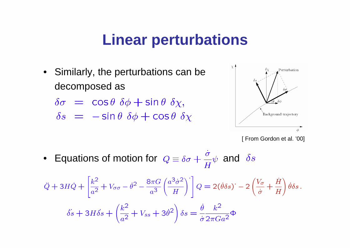
Linear perturbations
• Similarly, the perturbations can be decomposed as
• Equations of motion for and
[ From Gordon et al. ’00]
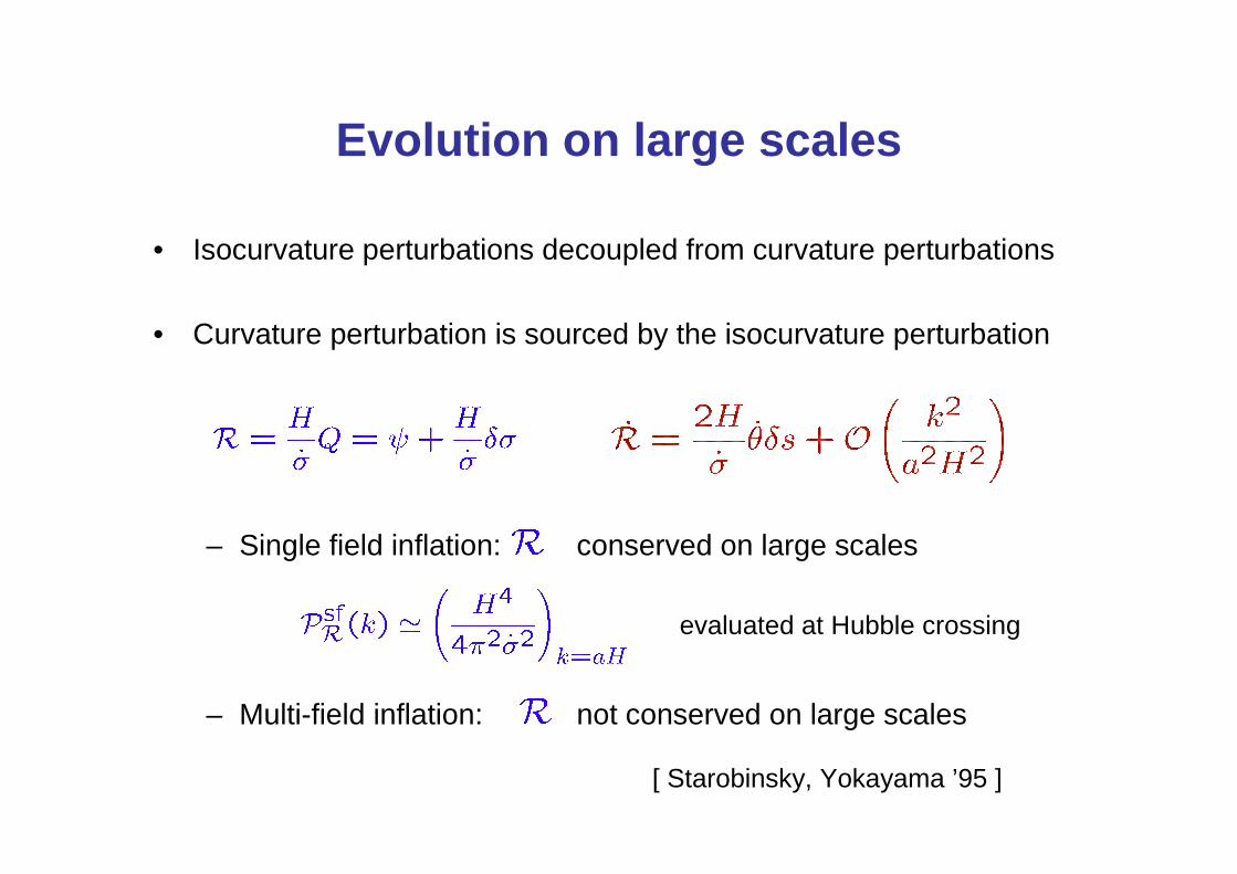
Evolution on large scales
• Isocurvature perturbations decoupled from curvature perturbations
• Curvature perturbation is sourced by the isocurvature perturbation
– Single field inflation: conserved on large scales
– Multi-field inflation: not conserved on large scales
evaluated at Hubble crossing
[ Starobinsky, Yokayama ’95 ]
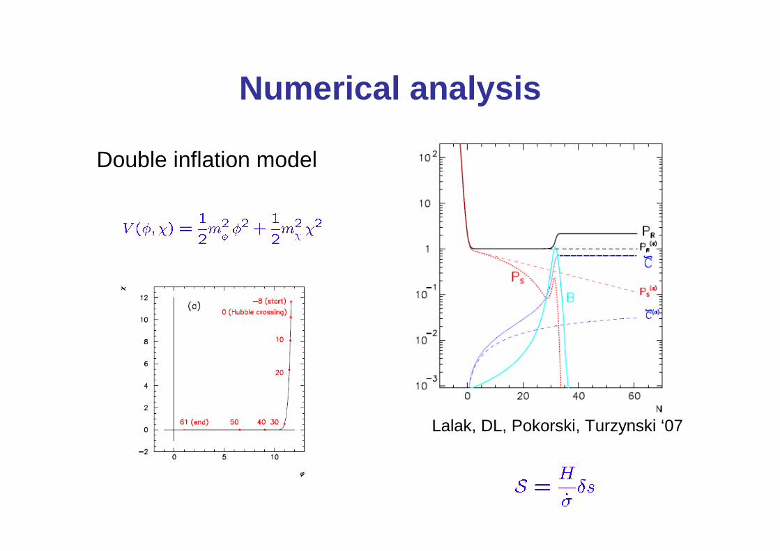
Numerical analysis
Double inflation model
Lalak, DL, Pokorski, Turzynski ‘07
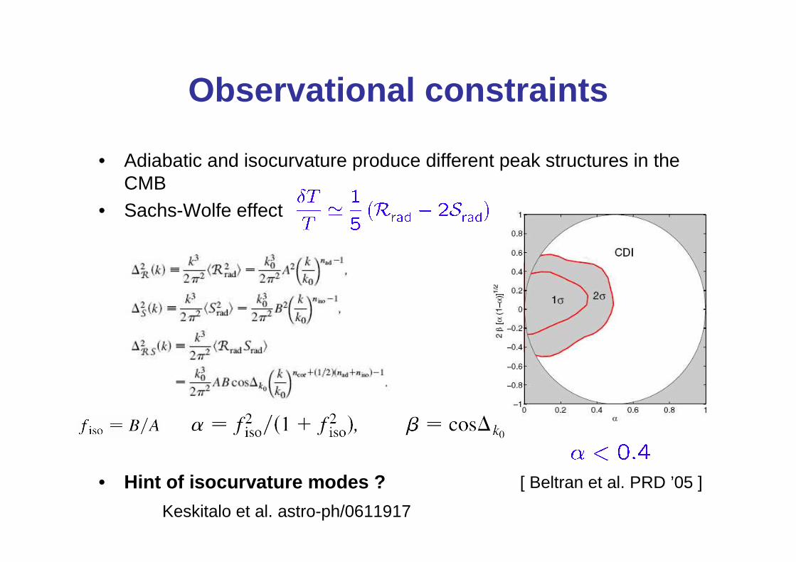
Observational constraints
• Adiabatic and isocurvature produce different peak structures in the CMB
• Sachs-Wolfe effect
• Hint of isocurvature modes ? [ Beltran et al. PRD ’05 ]
Keskitalo et al. astro-ph/0611917

The curvaton scenario
Light scalar field during inflation (when H > m)which later oscillates (when H < m), and finally decays.
Mollerach (1990); Linde & Mukhanov (1997) ;Enqvist & Sloth; Lyth & Wands; Moroi & Takahashi (2001)
Decay
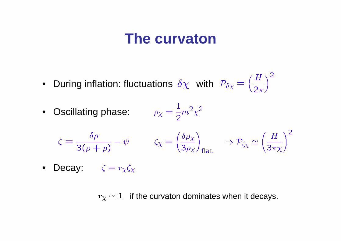
The curvaton
• During inflation: fluctuations with
• Oscillating phase:
• Decay:
if the curvaton dominates when it decays.
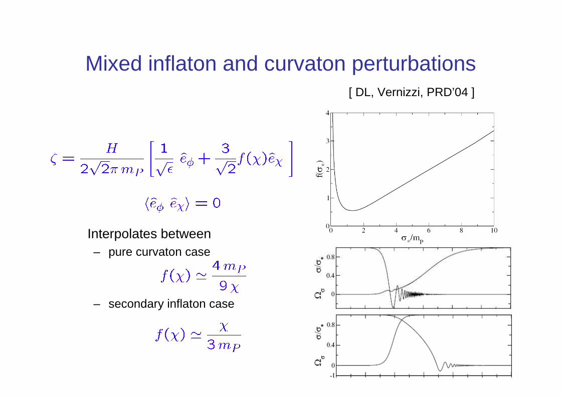
Mixed inflaton and curvaton perturbations
Interpolates between – pure curvaton case
– secondary inflaton case
[ DL, Vernizzi, PRD’04 ]
Conclusions
Multi-field inflation generates isocurvature perturbations in addition to adiabatic perturbations- Isocurvature perturbations affect the evolution of the curvature
perturbation (if the trajectory is bent).- Depending on the models (reheating), the isocurvature
perturbations can survive after inflation.- In this case, the primordial adiabatic and isocurvature are in
general correlated.- An isocurvature contribution in the primordial perturbations can
in principle be detected in cosmological observations.
additional window on the early universe physics


