Productivity performances in spruce plantations: DTW versus TWI comparison
This presentation details how height increments of spruce plantationsvary in relation to two rasterized LiDAR-DEM derived indicators of soilwetness / drainage (Slide 2), i.e.,
• the cartographic Depth-to-Water index DTW, referring to theelevational rise away from nearest streams and other surfacewater bodies, and
• the Terrain Wetness Index, referring to the logarithm of theupslope flow accumulation area over slope ratio at each rasterpixel.
Slide 3 shows how height increments within the JDI Black Brook ForestManagement area in New Brunswick vary with DTW and TWI by way of
• box plots, with DTW and TWI grouped by classes, and
• best-fitted regression plots
• the corresponding DTW-based equations for the resulting annualheight, basal area and total volume increments are shown on theright.
Slides 4 and 5 present an example area depicting the annual 90th
percentile height increments per 20x20 m cells (shown as dots)overlain on the DTW and TWI rasters. Slides 5 indicates that TWI, incontrast to DTW (Slide 4), is too detailed to correspond to the overallplantation growth pattern.
The conclusion is that elevation-induced differences in soil wetnessand drainage (as captured by log10DTW) away from flow channelsaffect plantation growth more than the log10-differences of upslopeflow accumulation over slope ratio (TWI).
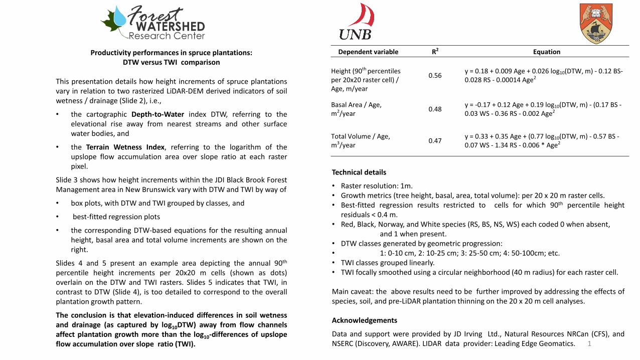
Dependent variable R2 Equation
Height (90th percentiles per 20x20 raster cell) / Age, m/year
0.56y = 0.18 + 0.009 Age + 0.026 log10(DTW, m) - 0.12 BS-0.028 RS - 0.00014 Age2
Basal Area / Age,m2/year
0.48y = -0.17 + 0.12 Age + 0.19 log10(DTW, m) - (0.17 BS -0.03 WS - 0.36 RS - 0.002 Age2
Total Volume / Age,m3/year
0.47y = 0.33 + 0.35 Age + (0.77 log10(DTW, m) - 0.57 BS -0.07 WS - 1.34 RS - 0.006 * Age2
Technical details
• Raster resolution: 1m.• Growth metrics (tree height, basal, area, total volume): per 20 x 20 m raster cells.• Best-fitted regression results restricted to cells for which 90th percentile height
residuals < 0.4 m.• Red, Black, Norway, and White species (RS, BS, NS, WS) each coded 0 when absent,
and 1 when present.• DTW classes generated by geometric progression:• 1: 0-10 cm, 2: 10-25 cm; 3: 25-50 cm; 4: 50-100cm; etc.• TWI classes grouped linearly.• TWI focally smoothed using a circular neighborhood (40 m radius) for each raster cell.
Main caveat: the above results need to be further improved by addressing the effects ofspecies, soil, and pre-LiDAR plantation thinning on the 20 x 20 m cell analyses.
Acknowledgements
Data and support were provided by JD Irving Ltd., Natural Resources NRCan (CFS), andNSERC (Discovery, AWARE). LIDAR data provider: Leading Edge Geomatics. 1

Definitions and Scatter Plot of TWI versus log10(DTW, m)
DTW: cartographic depth-to-water index, m:
TWI = log10upslope flow accumulation, ha
slope, %
Cartographic Water Table (DEM-DTW)
DEM
DTW
Soil drainage
excessive
moderate
very poor

3
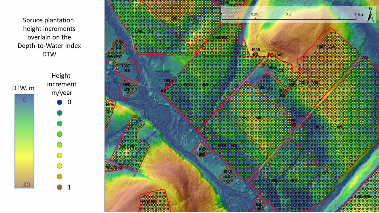
0 0.5 10.25 km ±Spruce plantation height increments
overlain on theDepth-to-Water Index
DTW
DTW, m
0
30
Height increment
m/year
0
1
4

TWI
6
2
Height increment
m/year
0
1
0 0.5 10.25 km ±Spruce plantation height increments
overlain on the Terrain Wetness Index
TWI
5

6
0.0 0.1 1.0 10.0 100.0
0.10
0.14
0.18
0.22
0.26
0.30
0.34
0.38
50th
90th
10th
25th
75th
Height IncrementPercentiles
m
DTW, m (x)
Hei
ght
incr
eme
nts
, m/y
ear
(y)
Model: y = a xb exp(-c x)
Statistical representation
of the cell-based height increment
overlay on the DTW raster in Slide 4,using curvilinear
regression analysis


