IntroductionThe Mathematics of Guarantee Options
The Optimization ModelImplementation and Results
Conclusions
Designing and pricing guarantee options in definedcontribution pension plans
Andrea Consiglio† Michele Tumminello† Stavros Zenios‡
†University of Palermo, IT‡University of Cyprus, CY
June 20166th International Conference
of the Financial Engineering and Banking Society
1 / 27
IntroductionThe Mathematics of Guarantee Options
The Optimization ModelImplementation and Results
Conclusions
Outline
1 Introduction
2 The Mathematics of Guarantee Options
3 The Optimization Model
4 Implementation and ResultsThe effect of policy parameters on the cost of the guaranteePortfolio composition, moral hazard and risk sharing
5 Conclusions
2 / 27
IntroductionThe Mathematics of Guarantee Options
The Optimization ModelImplementation and Results
Conclusions
Motivations and contributions
Retirement plans are of two types:
DB -Defined benefits plans shift the risks to the provider, be ita corporate employer or future taxpayersDC -Defined contributions plans pass the risks to retirees.
The retirement income must be “safe”:
DC politically acceptableEncourage participationIncrease savings
Some type of guarantee is needed and the success ofDC hinges upon the design of appropriate guarantees.
3 / 27

IntroductionThe Mathematics of Guarantee Options
The Optimization ModelImplementation and Results
Conclusions
Motivations and contributions / 2
Difficulty in designing the guarantee does not stop to thedefinition of its mechanism.
Guarantees provisions are written on asset portfolio, and thesedecisions need to be “optimised for their safety andperformance”. (European Commission 2012)
Given the complex interactions of financial, economic anddemographic risks, a guarantee may fail as much as a “definedbenefit” may be modified by government legislation.(World Bank 2000).
4 / 27

IntroductionThe Mathematics of Guarantee Options
The Optimization ModelImplementation and Results
Conclusions
Motivations and contributions / 3
Our contributions:1 Modelling DC plans with alternative guarantee options
2 Optimizing asset allocation to facilitate risk sharing
5 / 27

IntroductionThe Mathematics of Guarantee Options
The Optimization ModelImplementation and Results
Conclusions
Motivations and contributions / 3
Our contributions:1 Modelling DC plans with alternative guarantee options2 Optimizing asset allocation to facilitate risk sharing
5 / 27

IntroductionThe Mathematics of Guarantee Options
The Optimization ModelImplementation and Results
Conclusions
DB vs DC pension plans in the OECD countries
0
20
40
60
80
100
Chile
Czech
Rep
ublic
Estonia
Franc
e
Greec
e
Hunga
ry
Poland
Slovak
Rep
ublic
Sloven
ia
Denm
ark
Italy
Austra
lia (1
)
Mex
ico
New Z
ealan
d (1
)
Icelan
dSpa
in
United
Sta
tes (
2)
Turk
eyIsr
ael
Korea
Luxe
mbo
urg
(3)
Portu
gal
Canad
a (2
)
Germ
any
Finlan
d
Norway
Switzer
land
Defined Contribution Defined Benefit / Hybrid Mixed
6 / 27
IntroductionThe Mathematics of Guarantee Options
The Optimization ModelImplementation and Results
Conclusions
Type of guarantees
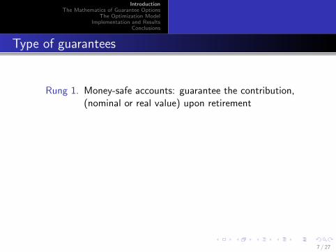
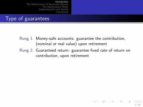
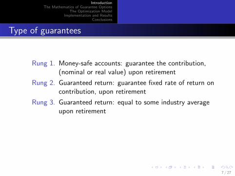
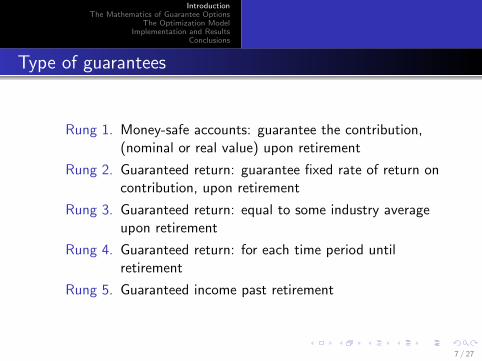
Rung 1. Money-safe accounts: guarantee the contribution,(nominal or real value) upon retirement
Rung 2. Guaranteed return: guarantee fixed rate of return oncontribution, upon retirement
Rung 3. Guaranteed return: equal to some industry averageupon retirement
Rung 4. Guaranteed return: for each time period untilretirement
Rung 5. Guaranteed income past retirement
7 / 27
IntroductionThe Mathematics of Guarantee Options
The Optimization ModelImplementation and Results
Conclusions
Type of guarantees
Rung 1. Money-safe accounts: guarantee the contribution,(nominal or real value) upon retirement
Rung 2. Guaranteed return: guarantee fixed rate of return oncontribution, upon retirement
Rung 3. Guaranteed return: equal to some industry averageupon retirement
Rung 4. Guaranteed return: for each time period untilretirement
Rung 5. Guaranteed income past retirement
7 / 27
IntroductionThe Mathematics of Guarantee Options
The Optimization ModelImplementation and Results
Conclusions
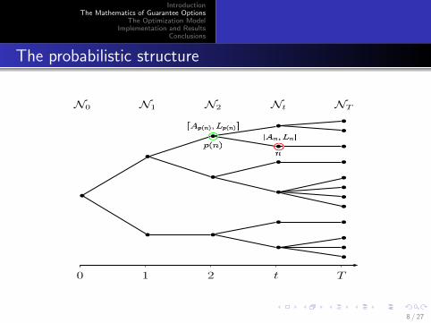
The probabilistic structure
Tt210
NTNtN2N1N0
8 / 27
IntroductionThe Mathematics of Guarantee Options
The Optimization ModelImplementation and Results
Conclusions
The basic minimum guarantee option
Model the minimum guarantee provision as an option writtenon a reference fund, with value An at time T for each n ∈ NT ;
We assume a closed fund with initial contribution L0 andregulatory equity requirement E0 = (1− α)A0, α < 1
L0 = αA0 and A0 = L0 + E0
A0 is invested in a reference portfolio with proportions xj , and∑j∈J xj = 1.
9 / 27
IntroductionThe Mathematics of Guarantee Options
The Optimization ModelImplementation and Results
Conclusions
The dynamics of the asset and liability account
Given a family of stochastic processes {Rt}t∈T defined as aJ-dimensional vector of returns, Rn ≡
(R1n , . . . ,R
Jn
)
The asset account for each n ∈ N\{0} is
An = Ap(n)eRAn
whereRAn =
∑j∈J
xjRjn
The liability account is Ln = Lp(n) exp[g + max
(δRA
n − g , 0)]
10 / 27

IntroductionThe Mathematics of Guarantee Options
The Optimization ModelImplementation and Results
Conclusions
The dynamics of the asset and liability account
Given a family of stochastic processes {Rt}t∈T defined as aJ-dimensional vector of returns, Rn ≡
(R1n , . . . ,R
Jn
)The asset account for each n ∈ N\{0} is
An = Ap(n)eRAn
whereRAn =
∑j∈J
xjRjn
The liability account is Ln = Lp(n) exp[g + max
(δRA
n − g , 0)]
10 / 27

IntroductionThe Mathematics of Guarantee Options
The Optimization ModelImplementation and Results
Conclusions
The objective function
We assume that shareholders cover shortfalls
A rational strategy for the fund manager is to minimize theexpected value of shortfalls:
Γ = e−rT∑n∈NT
qn max (Ln − An, 0)]
where the qn are the risk neutral probabilities.
The cost of the guarantee is the cost of a put optionwritten on the value of the asset An with a stochasticstrike price Ln
11 / 27

IntroductionThe Mathematics of Guarantee Options
The Optimization ModelImplementation and Results
Conclusions
Bilinear constraints
Denote by wn and zn the final cumulative returns of the assetand liability accounts An and Ln.For all n ∈ NT , we have:
wn =∑
i∈P(n)
RAi ,
zn =∑
i∈P(n)
g + max(δRA
i − g , 0),
Discontinuous nonlinear programming problem (DNLP)
12 / 27

IntroductionThe Mathematics of Guarantee Options
The Optimization ModelImplementation and Results
Conclusions
Bilinear constraints / 2
Introduce the set of equations to define the max operator:
δRAn − g = ε+
n − ε−n ,ε+n ε−n = 0,
ε+n , ε
−n ≥ 0.
13 / 27
IntroductionThe Mathematics of Guarantee Options
The Optimization ModelImplementation and Results
Conclusions
Bilinear constraints / 3
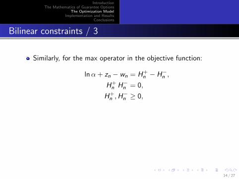
Similarly, for the max operator in the objective function:
lnα + zn − wn = H+n − H−n ,
H+n H−n = 0,
H+n ,H
−n ≥ 0,
The cost of the guarantee becomes:
Γ(x1, x2, . . . , xJ) = e−rTA0
∑n∈NT
qnewn
(eH
+n − 1
).
14 / 27

IntroductionThe Mathematics of Guarantee Options
The Optimization ModelImplementation and Results
Conclusions
Bilinear constraints / 3
Similarly, for the max operator in the objective function:
lnα + zn − wn = H+n − H−n ,
H+n H−n = 0,
H+n ,H
−n ≥ 0,
The cost of the guarantee becomes:
Γ(x1, x2, . . . , xJ) = e−rTA0
∑n∈NT
qnewn
(eH
+n − 1
).
14 / 27
IntroductionThe Mathematics of Guarantee Options
The Optimization ModelImplementation and Results
Conclusions
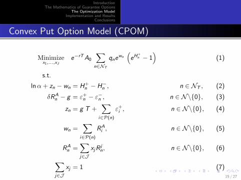
Convex Put Option Model (CPOM)
Minimizex1,...,xJ
e−rTA0
∑n∈NT
qnewn
(eH
+n − 1
)(1)
s.t.
lnα + zn − wn = H+n − H−n , n ∈ NT , (2)
δRAn − g = ε+
n − ε−n , n ∈ N\{0}, (3)
zn = g T +∑
i∈P(n)
ε+i , n ∈ N\{0}, (4)
wn =∑
i∈P(n)
RAi , n ∈ N\{0}, (5)
RAn =
∑j∈J
xjRjn, n ∈ N\{0}, (6)
∑j∈J
xj = 1 (7)
15 / 27

IntroductionThe Mathematics of Guarantee Options
The Optimization ModelImplementation and Results
Conclusions
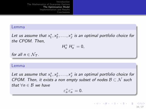
Lemma
Let us assume that x∗1 , x∗2 , . . . , x
∗J is an optimal portfolio choice for
the CPOM. Then,H+n H−n = 0,
for all n ∈ NT .
Lemma
Let us assume that x∗1 , x∗2 , . . . , x
∗J is an optimal portfolio choice for
CPOM. Then, it exists a non empty subset of nodes B ⊂ N suchthat ∀n ∈ B we have
ε+n ε−n = 0.
16 / 27
IntroductionThe Mathematics of Guarantee Options
The Optimization ModelImplementation and Results
Conclusions
Lemma
Let us assume that x∗1 , x∗2 , . . . , x
∗J is an optimal portfolio choice for
the CPOM. Then,H+n H−n = 0,
for all n ∈ NT .
Lemma
Let us assume that x∗1 , x∗2 , . . . , x
∗J is an optimal portfolio choice for
CPOM. Then, it exists a non empty subset of nodes B ⊂ N suchthat ∀n ∈ B we have
ε+n ε−n = 0.
16 / 27

IntroductionThe Mathematics of Guarantee Options
The Optimization ModelImplementation and Results
Conclusions
Corollary
Let x∗1 , x∗2 , . . . , x
∗J be an optimal portfolio choice for the CPOM, if
ε+k ε−k > 0, for any k ∈ N , then it exists n ∈ NT such that
k ∈ P(n) andH−n > 0 or H−n = H+
n = 0.
Theorem
Let x∗1 , x∗2 , . . . , x
∗J be an optimal portfolio choice for the CPOM,
with optimal objective value Γ∗. Let x∗∗1 , x∗∗2 , . . . , x∗∗J be anoptimal portfolio choice of the NCPOM, with optimal objectivevalue Γ∗∗. Then
Γ∗ = Γ∗∗.
17 / 27

IntroductionThe Mathematics of Guarantee Options
The Optimization ModelImplementation and Results
Conclusions
The effect of policy parameters on the cost of the guaranteePortfolio composition, moral hazard and risk sharing
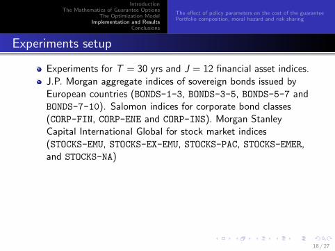
Experiments setup
Experiments for T = 30 yrs and J = 12 financial asset indices.
J.P. Morgan aggregate indices of sovereign bonds issued byEuropean countries (BONDS-1-3, BONDS-3-5, BONDS-5-7 andBONDS-7-10). Salomon indices for corporate bond classes(CORP-FIN, CORP-ENE and CORP-INS). Morgan StanleyCapital International Global for stock market indices(STOCKS-EMU, STOCKS-EX-EMU, STOCKS-PAC, STOCKS-EMER,and STOCKS-NA)Data from FINLIB(Zenios, Practical Financial Optimization. Decision makingfor financial engineers, Blackwell-Wiley Finance, 2007)Simulate risk-neutral process of asset returns using standardMontecarlo approachModel implemented simulating fan of 1000 risk-neutral paths
18 / 27
IntroductionThe Mathematics of Guarantee Options
The Optimization ModelImplementation and Results
Conclusions
The effect of policy parameters on the cost of the guaranteePortfolio composition, moral hazard and risk sharing
Experiments setup
Experiments for T = 30 yrs and J = 12 financial asset indices.J.P. Morgan aggregate indices of sovereign bonds issued byEuropean countries (BONDS-1-3, BONDS-3-5, BONDS-5-7 andBONDS-7-10). Salomon indices for corporate bond classes(CORP-FIN, CORP-ENE and CORP-INS). Morgan StanleyCapital International Global for stock market indices(STOCKS-EMU, STOCKS-EX-EMU, STOCKS-PAC, STOCKS-EMER,and STOCKS-NA)
Data from FINLIB(Zenios, Practical Financial Optimization. Decision makingfor financial engineers, Blackwell-Wiley Finance, 2007)Simulate risk-neutral process of asset returns using standardMontecarlo approachModel implemented simulating fan of 1000 risk-neutral paths
18 / 27

IntroductionThe Mathematics of Guarantee Options
The Optimization ModelImplementation and Results
Conclusions
The effect of policy parameters on the cost of the guaranteePortfolio composition, moral hazard and risk sharing
Experiments setup
Experiments for T = 30 yrs and J = 12 financial asset indices.J.P. Morgan aggregate indices of sovereign bonds issued byEuropean countries (BONDS-1-3, BONDS-3-5, BONDS-5-7 andBONDS-7-10). Salomon indices for corporate bond classes(CORP-FIN, CORP-ENE and CORP-INS). Morgan StanleyCapital International Global for stock market indices(STOCKS-EMU, STOCKS-EX-EMU, STOCKS-PAC, STOCKS-EMER,and STOCKS-NA)Data from FINLIB(Zenios, Practical Financial Optimization. Decision makingfor financial engineers, Blackwell-Wiley Finance, 2007)
Simulate risk-neutral process of asset returns using standardMontecarlo approachModel implemented simulating fan of 1000 risk-neutral paths
18 / 27

IntroductionThe Mathematics of Guarantee Options
The Optimization ModelImplementation and Results
Conclusions
The effect of policy parameters on the cost of the guaranteePortfolio composition, moral hazard and risk sharing
Experiments setup
Experiments for T = 30 yrs and J = 12 financial asset indices.J.P. Morgan aggregate indices of sovereign bonds issued byEuropean countries (BONDS-1-3, BONDS-3-5, BONDS-5-7 andBONDS-7-10). Salomon indices for corporate bond classes(CORP-FIN, CORP-ENE and CORP-INS). Morgan StanleyCapital International Global for stock market indices(STOCKS-EMU, STOCKS-EX-EMU, STOCKS-PAC, STOCKS-EMER,and STOCKS-NA)Data from FINLIB(Zenios, Practical Financial Optimization. Decision makingfor financial engineers, Blackwell-Wiley Finance, 2007)Simulate risk-neutral process of asset returns using standardMontecarlo approach
Model implemented simulating fan of 1000 risk-neutral paths
18 / 27

IntroductionThe Mathematics of Guarantee Options
The Optimization ModelImplementation and Results
Conclusions
The effect of policy parameters on the cost of the guaranteePortfolio composition, moral hazard and risk sharing
Experiments setup
Experiments for T = 30 yrs and J = 12 financial asset indices.J.P. Morgan aggregate indices of sovereign bonds issued byEuropean countries (BONDS-1-3, BONDS-3-5, BONDS-5-7 andBONDS-7-10). Salomon indices for corporate bond classes(CORP-FIN, CORP-ENE and CORP-INS). Morgan StanleyCapital International Global for stock market indices(STOCKS-EMU, STOCKS-EX-EMU, STOCKS-PAC, STOCKS-EMER,and STOCKS-NA)Data from FINLIB(Zenios, Practical Financial Optimization. Decision makingfor financial engineers, Blackwell-Wiley Finance, 2007)Simulate risk-neutral process of asset returns using standardMontecarlo approachModel implemented simulating fan of 1000 risk-neutral paths
18 / 27

IntroductionThe Mathematics of Guarantee Options
The Optimization ModelImplementation and Results
Conclusions
The effect of policy parameters on the cost of the guaranteePortfolio composition, moral hazard and risk sharing
Minimum guarantee rate (g)
Min
imum
gua
rant
ee c
ost
0.0
0.5
1.0
1.5
2.0
2.5
0
0.01
0.02
0.03
0.04
0.05
0.7
0
0.01
0.02
0.03
0.04
0.05
0.8
0
0.01
0.02
0.03
0.04
0.05
1
alpha0.7 0.8 1
19 / 27
IntroductionThe Mathematics of Guarantee Options
The Optimization ModelImplementation and Results
Conclusions
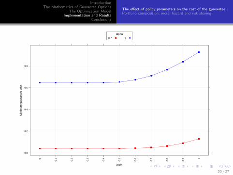
The effect of policy parameters on the cost of the guaranteePortfolio composition, moral hazard and risk sharing
delta
Min
imum
gua
rant
ee c
ost
0.0
0.2
0.4
0.6
0.8
0
0.1
0.2
0.3
0.4
0.5
0.6
0.7
0.8
0.9 1
alpha0.7 1
20 / 27
IntroductionThe Mathematics of Guarantee Options
The Optimization ModelImplementation and Results
Conclusions
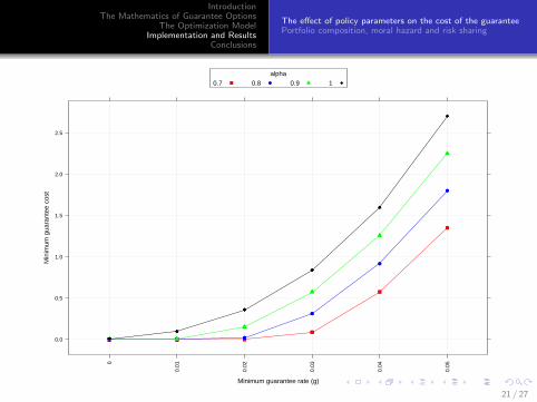
The effect of policy parameters on the cost of the guaranteePortfolio composition, moral hazard and risk sharing
Minimum guarantee rate (g)
Min
imum
gua
rant
ee c
ost
0.0
0.5
1.0
1.5
2.0
2.5
0
0.01
0.02
0.03
0.04
0.05
alpha0.7 0.8 0.9 1
21 / 27

IntroductionThe Mathematics of Guarantee Options
The Optimization ModelImplementation and Results
Conclusions
The effect of policy parameters on the cost of the guaranteePortfolio composition, moral hazard and risk sharing
Portfolio percentages
BONDS_1_3
CORP_FIN
CORP_INS
STOCKS_EMER
STOCKS_EMU
STOCKS_PAC
0.0 0.2 0.4 0.6 0.8
0.7
0.0 0.2 0.4 0.6 0.8
0.9
g0 0.01 0.03 0.05
22 / 27

IntroductionThe Mathematics of Guarantee Options
The Optimization ModelImplementation and Results
Conclusions
The effect of policy parameters on the cost of the guaranteePortfolio composition, moral hazard and risk sharing
Years
Year
ly r
etur
ns (
%)
−40
−20
0
20
40
1995 2000 2005 2010
10−Year T−Bond 3−Month T−Bill
Portfolio
1995 2000 2005 2010
−40
−20
0
20
40S&P500
23 / 27
IntroductionThe Mathematics of Guarantee Options
The Optimization ModelImplementation and Results
Conclusions
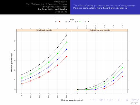
The effect of policy parameters on the cost of the guaranteePortfolio composition, moral hazard and risk sharing
Minimum guarantee rate (g)
Min
imum
gua
rant
ee c
ost
0
1
2
3
4
5
0
0.01
0.02
0.03
0.04
0.05
Benchmark portfolio
0 0.01
0.02
0.03
0.04
0.05
Optimal reference portfolio
alpha0.7 0.8 0.9 1
24 / 27
IntroductionThe Mathematics of Guarantee Options
The Optimization ModelImplementation and Results
Conclusions
The effect of policy parameters on the cost of the guaranteePortfolio composition, moral hazard and risk sharing
Risk Sharing
Cost of guarantee can be used to set risk sharing premia.E.g., for g=3% and α = 1 (zero equity) we have cost 0.84.
Case 1. The pension fund bears the risk of the guarantee. Thebeneficiary will pay 1.84 and will get a return only on 1 euro.
Case 2. Risk sharing between the beneficiary and a thirdparty. For example, the cost of sharing consist in paying 0.3 ofequity (α = 0.7), and investing it in the reference portfolio.The cost of the guarantee is 0.09.
25 / 27

IntroductionThe Mathematics of Guarantee Options
The Optimization ModelImplementation and Results
Conclusions
Concluding remarks
A general and computationally tractable model for pricing thecost of alternative embedded guarantee options in DC pensionfunds.
Model to determine the asset allocation choice that is optimalfor a given guarantee, in that it minimizes the cost of theguarantee.
Can be used to benchmark existing portfolios by applying it totest portfolios of State and local government pension funds.
Can be used to calculate risk premia for risk sharing.
26 / 27
IntroductionThe Mathematics of Guarantee Options
The Optimization ModelImplementation and Results
Conclusions
Reference
A. Consiglio, M. Tumminlello and S.A. Zenios, Designing andpricing guarantee options in defined contributions pension plans,Insurance: Mathematics and Economics, 65:267–279, 2015.
27 / 27


