DEVELOPING A FOUR-BAR MECHANISM SYNTHESIS PROGRAM
IN CAD ENVIRONMENT
A THESIS SUBMITTED TO THE GRADUATE SCHOOL OF NATURAL AND APPLIED SCIENCES
OF MIDDLE EAST TECHNICAL UNIVERSITY
BY
KAAN ERENER
IN PARTIAL FULFILLMENT OF THE REQUIREMENTS FOR
THE DEGREE OF MASTER OF SCIENCE IN
MECHANICAL ENGINEERING
JUNE 2011
Approval of the thesis:
DEVELOPING A FOUR-BAR MECHANISM SYNTHESIS PROGRAM IN
CAD ENVIRONMENT
submitted by Kaan ERENER in partial fulfillment of the requirements for the
degree of Master of Science in Mechanical Engineering Department, Middle
East Technical University by,
Prof. Dr. Canan Özgen Dean, Graduate School of Natural and Applied Sciences Prof. Dr. Süha Oral Head of Department, Mechanical Engineering Prof. Dr. Eres Söylemez Supervisor, Mechanical Engineering Dept., METU Examining Committee Members: Prof. Dr. Reşit Soylu Mechanical Engineering Dept., METU Prof. Dr. Eres Söylemez Mechanical Engineering Dept., METU Asst. Prof. Dr. Ergin Tönük Mechanical Engineering Dept., METU Asst. Prof. Dr. Gökhan Özgen Mechanical Engineering Dept., METU Süleyman Yangınlar Mechanical and Hydraulic Systems Chief, TAI
Date:

iii
I hereby declare that all information in this document has been obtained and presented in accordance with academic rules and ethical conduct. I also declare that, as required by these rules and conduct, I have fully cited and referenced all material and results that are not original to this work.
Name, Last Name: Kaan ERENER
Signature:

iv
ABSTRACT
DEVELOPING A FOUR BAR MECHANISM SYNTHESIS PROGRAM
IN CAD ENVIRONMENT
Erener, Kaan
M.Sc., Department of Mechanical Engineering
Supervisor: Prof. Dr. Eres Söylemez
June 2011, 78 pages
Flap, aileron, rudder, elevator, speed brake, stick, landing gear and similar movable
systems used in aerospace industry have to operate according to the defined
requirements and mechanisms used in those systems have to be synthesized in order
to fulfill those requirements. Generally, without the use of synthesis tools, synthesis
of mechanisms are done in CAD environment by trial-error and geometrical methods
due to the complexity of analytical procedures. However, this approach is time
consuming since it has to be repeated until the synthesized mechanism has suitable
mechanism properties like transmission angle and connection points. Due to above
reasons, a software developed for synthesis of mechanisms within the CAD
environment can utilize all the graphical interfaces and provides convenience in
mechanism design.
In this work, it is aimed to develop a four-bar mechanism synthesis tool which is
compatible with CATIA V5 by considering the requirements of aerospace industry.

v
This tool performs function, path and motion synthesis and shows suitable
mechanisms in CATIA according to input obtained from CATIA and mechanism
properties.
Keywords: Mechanism Synthesis, Four-bar, Burmester Theory, CAD, CATIA

vi
ÖZ
CAD ORTAMINDA DÖRT ÇUBUK MEKANİZMASI SENTEZLEME
PROGRAMI GELİŞTİRİLMESİ
Erener, Kaan
Yüksek Lisans, Makine Mühendisliği Bölümü
Tez Yöneticisi: Prof. Dr. Eres Söylemez
Haziran 2011, 78 sayfa
Havacılık sektöründe kullanılan flap, kanatçık, kuyruk ve irtifa dümeni, hız freni,
levye, iniş takımları ve benzeri hareketli sistemlerin belli isterler doğrultusunda
çalışabilmesi için kullanılacak olan mekanizmaların bu doğrultuda sentezlerinin
gerçekleştirilmesi gerekmektedir. Bu mekanizmalar, sentez yazılımlarının
kullanılmadığı durumlarda, analitik işlemlerin karmaşıklığı nedeniyle, genel olarak
CAD programlarında deneme-yanılma ve geometrik metotlarla sentezlenmektedir.
Ancak, bu sürecin oluşturulan mekanizmanın bağlantı noktaları ve bağlama açısı gibi
mekanizma özellikleri uygun oluncaya kadar tekrarlanması zaman kaybına neden
olmaktadır. Bu nedenlerden ötürü, mekanizma sentezini, CAD programlarının grafik
arayüzlerini kullanarak gerçekleştiren bir yazılım, mekanizma tasarımlarında
kolaylık sağlayacaktır.
Bu çalışmada, havacılık sektörünün gereksinimleri ön planda tutularak CATIA V5
programı ile birlikte çalışabilen, dört çubuk mekanizma sentezleme programının

vii
geliştirilmesi amaçlanmıştır. Bu program, CATIA’dan aldığı girdilerle, konum,
yörünge ve fonksiyon sentezlerini gerçekleştirebilen ve istenilen mekanizma
özelliklerine göre uygun mekanizma alternatiflerini yine CATIA’da çıktı olarak
gösterebilme özelliklerine sahiptir.
Anahtar Kelimeler: Mekanizma Sentezi, Dört Çubuk, Burmester Teorisi, CAD,
CATIA

viii
ACKNOWLEDGEMENTS
I would like to thank my supervisor, Prof. Dr. Eres Söylemez, for his continuos
support and motivation during the thesis project.
I thank my employers and colleagues at Turkish Aerospace Industry for their support
and nice working environment.
Finally, I would like to thank my parents Şükran and Hüseyin Erener, my sister
Şüheda for unconditional love, support and encouragement and a very special thank
to Gözde for her love, comfort, support and bearing with me.

ix
TABLE OF CONTENTS
ABSTRACT………………………………………………………………………….iv
ÖZ…………………………...……………...……………………………….……….vi
ACKNOWLEDGEMENTS………………………………………………………...viii
TABLE OF CONTENTS…………………………………...………………………..ix
LIST OF FIGURES……………………………………..………………….………..xi
LIST OF TABLES………………………………………………...........…………..xiii
CHAPTERS
1. INTRODUCTION ................................................................................................ 1
1.1 GENERAL .................................................................................................... 1
1.2 LITERATURE SURVEY ............................................................................. 3
2. THEORY AND FORMULATION ...................................................................... 8
2.1 GENERAL .................................................................................................... 8
2.2 MULTIPLY SEPARATED POSITION AND DYADIC APROACH ....... 11
2.3 SYNTHESIS TASKS .................................................................................. 15
2.3.1 Synthesis for Motion Generation ......................................................... 15
2.3.2 Synthesis for Path Generation .............................................................. 20
2.3.3 Synthesis for Function Generation ....................................................... 20
2.4 DEFECTS IN MECHANISM SYNTHESIS .............................................. 22
2.5 SPECIAL CASES ....................................................................................... 23
2.5.1 Case P-P-P ............................................................................................ 23
2.5.2 Case P-P-P-P ........................................................................................ 25
2.5.3 Case PP-P-P ......................................................................................... 26
2.5.4 Case PPPP ............................................................................................ 26
2.6 SynCAT ....................................................................................................... 27
x
2.6.1 Usage .................................................................................................... 27
2.6.2 Interface between CATIA and SynCAT .............................................. 31
3. MECHANISM SYNTHESIS PROBLEMS AND SOLUTIONS ...................... 32
3.1 NOSE LANDING GEAR DOOR MECHANISM ...................................... 32
3.1.1 Problem Definition ............................................................................... 32
3.1.2 Problem Solution (P-P-P-P Alternative – 1) ........................................ 33
3.1.3 Problem Solution (PP-P-P Alternative – 2) ......................................... 39
3.1.4 Problem Solution (PPP-P Alternative – 3) ........................................... 42
3.2 FLAP CONTROL SURFACE MECHANISM ........................................... 44
3.2.1 Problem Definition ............................................................................... 44
3.2.2 Problem Solution .................................................................................. 45
3.3 PRIMARY CONTROL SURFACE MECHANISMS ................................ 51
3.3.1 Problem Definition ............................................................................... 51
3.3.2 Problem Solution .................................................................................. 53
3.4 ACCESS DOOR MECHANISM ................................................................ 57
3.4.1 Problem Definition ............................................................................... 57
3.4.2 Problem Solution .................................................................................. 58
3.5 MISCELLANEOUS TYPES OF MECHANISMS ..................................... 62
3.5.1 Approximation of a straight line .......................................................... 62
3.5.2 Correlation of crank angles .................................................................. 66
4. DISCUSSION AND CONCLUSION ................................................................ 69
4.1 SUMMARY AND DISCUSSION .............................................................. 69
4.2 FUTURE WORKS ...................................................................................... 70
REFERENCES ........................................................................................................... 71
APPENDICES
A: FLOWCHART OF SynCAT ......................................................................... 75
B: OBTAINING COORDINATES OF A POINT FROM CATIA ................... 76
C: PRINTING POINT ONTO CATIA ............................................................... 77
D: PRINTING LINE ONTO CATIA ................................................................. 78

xi
LIST OF FIGURES
FIGURES Figure 1 Illustrations for motion, path and function generation .................................. 2 Figure 2 Motion of a moving plane respect to fixed frame.......................................... 9 Figure 3 Fixed and moving centrode curves .............................................................. 11 Figure 4 Dyadic representation of four-bar mechanism ............................................ 12 Figure 5 SynCAT synthesis generation types ............................................................ 28 Figure 6 SynCAT function generation MSP types .................................................... 28 Figure 7 SynCAT design parameter entrance screen ................................................. 29 Figure 8 SynCAT mechanism properties entrance screen ......................................... 30 Figure 9 View of SynCAT output in CATIA screen ................................................. 30 Figure 10 General representation for NLG ................................................................ 32 Figure 11 Suitable regions for circle and center points.............................................. 34 Figure 12 Input screen for P-P-P-P function generation ............................................ 34 Figure 13 Burmester curve alternatives for NLG door mechanism ........................... 35 Figure 14 Design criteria entrance screen .................................................................. 35 Figure 15 Result of suitable output links ................................................................... 36 Figure 16 Selected output link and constructed mechanism ...................................... 36 Figure 17 Kinematic analysis of selected mechanism ............................................... 37 Figure 18 Input screen for PP-P-P function generation ............................................. 39 Figure 19 Result of suitable output links ................................................................... 40 Figure 20 Angular position relation of selected mechanism ...................................... 40 Figure 21 Angular velocity relation of selected mechanism ...................................... 41 Figure 22 Kinematic analysis of obtained mechanism .............................................. 41 Figure 23 Input screen for PPP-P function generation............................................... 42 Figure 24 Result of suitable output links ................................................................... 43 Figure 25 Kinematic analysis of obtained mechanism .............................................. 43 Figure 26 General view of flap control surface ......................................................... 45 Figure 27 Problem schematic ..................................................................................... 46 Figure 28 Input screen for P-P-P-P motion generation .............................................. 46
xii
Figure 29 Cross-sectional view of flap control surface and interested regions ......... 47 Figure 30 Suitable points for moving and fixed points .............................................. 47 Figure 31 Design criteria entrance screen .................................................................. 48 Figure 32 Output link alternatives for selected input link .......................................... 49 Figure 33 Kinematic analysis of selected mechanism ............................................... 49 Figure 34 Motion demonstration of obtained mechanism ......................................... 50 Figure 35 General scheme for elevator control system .............................................. 51 Figure 36 Suitable regions for circle and center points.............................................. 53 Figure 37 Input screen for P-P-P-P function generation ............................................ 54 Figure 38 Design criteria entrance screen .................................................................. 54 Figure 39 Suitable output links according to the selected input link ......................... 55 Figure 40 Suitable region for center and circle points ............................................... 55 Figure 41 Input screen for P-P-P-P function generation ............................................ 56 Figure 42 Design criteria entrance screen .................................................................. 56 Figure 43 Suitable cranks for obtained link ............................................................... 56 Figure 44 Demonstration of motion of mechanism ................................................... 57 Figure 45 Dead-center configuration for four-bar ..................................................... 58 Figure 46 Open configuration for access panel ......................................................... 59 Figure 47 Closed configuration for access panel ....................................................... 59 Figure 48 Suitable regions for center and circle points.............................................. 60 Figure 49 Input screen for PP-P-P function generation ............................................. 60 Figure 50 Suitable cranks for selected link ................................................................ 61 Figure 51 Kinematic analysis of obtained mechanism .............................................. 62 Figure 52 Input screen for PPPP motion generation .................................................. 64 Figure 53 Center and Circle points for desired mechanism ....................................... 64 Figure 54 Mechanism properties entrance screen ...................................................... 65 Figure 55 Suitable cranks according to the selected fixed point ................................ 65 Figure 56 Constructed mechanism and straight line path .......................................... 66 Figure 57 Epicyclic gear train .................................................................................... 66 Figure 58 Input entrance screen for PPPP function generation ................................. 67 Figure 59 Center and Circle points for desired mechanism ....................................... 68 Figure 60 Constructed mechanism and correlation between rotation angles ............. 68 Figure 61 Flowchart of SynCAT ............................................................................... 75

xiii
LIST OF TABLES
TABLES Table 1 Representation for finitely and infinitesimally separated positions .............. 12 Table 2 Notations for prescribed position .................................................................. 13 Table 3 The specified parameters for motion generation........................................... 15 Table 4 Explicit terms used in the dyad loop equation for three positions ................ 17 Table 5 Coefficients of the dyad loop equations for MSP motion generation ........... 20 Table 6 Special cases for P-P-P ................................................................................. 24 Table 7 Special cases for P-P-P-P .............................................................................. 25 Table 8 Special cases for PP-P-P ............................................................................... 26 Table 9 Crank rotation correlations for SynCAT for alternative-1 ............................ 33 Table 10 Motion demonstration of obtained mechanism ........................................... 37 Table 11 Crank rotation correlations for SynCAT for alternative-2 .......................... 39 Table 12 Crank rotation correlations for SynCAT for alternative-3 .......................... 42 Table 13 Desired flap rotations .................................................................................. 44 Table 14 Flap rotations input for SynCAT ................................................................ 45 Table 15 First mechanism design input ..................................................................... 52 Table 16 Second mechanism design input ................................................................. 52 Table 17 Summary of the desired motion of mechanism .......................................... 53 Table 18 Input for SynCAT ....................................................................................... 60
1
CHAPTER 1
1. INTRODUCTION
1.1 GENERAL
Kinematic synthesis of mechanism is one of the essential steps of the machine
design. According to the duty of machine, several types of mechanisms can be
synthesized and largely number of different configurations can be found. After the
type of mechanism is determined, the dimensional synthesis has to be performed.
Prescribed position synthesis is the most common method for dimensional synthesis
and this is the basis of this thesis subject.
The prescribed position synthesis is commonly divided into three parts. These are
namely, motion generation, path generation and function generation. Motion
generation deals with rotation and translation of a body while it passes from several
positions. Path generation deals only translation of a point and function generation is
about correlation of input and output motion.
For all these tasks, two curves are obtained which satisfies the prescribed positions
namely center and circle point locus. These loci show the fixed and moving pivots of
the suitable mechanism respectively.
In mechanism synthesis, if the design conditions are suitable, there are an infinite
number of solutions and it is engineer’s ability to judge and select suitable
mechanism type and configuration. Even though various analytical methods have
been developed for synthesis of mechanisms, it still depends on trial-error and
repetitive tasks which causes loss of time and money.

2
Motion Generation
Path Generation
Function Generation
Figure 1 Illustrations for motion, path and function generation
Today, there is a need to reduce cost and save time for early stages of design namely
for preliminary design. Therefore, a program which synthesizes mechanism
according to user inputs and does trial-error for numerous requirements and
conditions will be advantageous especially for aerospace industries which have lots
of requirements and conditions.
The aim of this thesis is to create visual and interactive computer software package
which works with CATIA V5 in fully parametric form and to apply this software
package in aircraft mechanisms design. The ability of program is planned to cover
3
motion synthesis, function generation and path synthesis of planar four-bar
mechanisms. Moreover, in order to satisfy possible requirement; velocity,
acceleration and transmission angle analysis shall be included in the program.
Since Visual Basic macros can be run under CATIA V5, the software is written in
Visual Basic environment, with graphical user interface for ease of usage.
1.2 LITERATURE SURVEY
The history of machine design goes back to 300 B.C. However, with the studies of
Ampere who excluded forces from kinematic analysis and studies of Reuleaux in
which mechanisms are classified (type synthesis) and their symbolic representations
are identified, “Kinematics” developed into a separate discipline in the 19th century.
Gruebler worked on number synthesis and developed criteria for the mobility of a
mechanism and in the end of 19th century, Burmester contributed on dimensional
synthesis by introducing the precision position concept. He used geometrical
methods and his work is known as Burmester Theory. [9, 21, 26]
After Burmester Theory, valuable contributions were done in synthesis of
mechanism by geometrical methods in the beginning of 20th century. Hartenberg
[18], in his textbook, considered both techniques namely analytical and graphical
approaches and used kinematic inversion and center point method as a geometrical
method for function and motion generation synthesis of mechanism with three and
four accuracy points. He defined the geometrical method as quick and staying close
to the physical problem but tedious for repetitive tasks. Moreover, Hall [16] used
geometrical method for synthesis of mechanism up to five specified position. In
addition to Hartenberg and Hall, Harrisberger [17] worked on geometrical methods
and used overlay method for synthesis of function generation, center point method
for synthesis of motion generation, catalog, center point and inflection circle methods
for synthesis for path generation.

4
After 50 years later from Burmester Theory, Ferdinand Freudenstein who is known
as “father of modern kinematics” developed an analytical approach to finitely
separated prescribed position concept [14]. With the help of this approach, he
introduced digital computation in the kinematic synthesis which reduced the
importance of trial-error and geometrical approaches [9]. Erdman and Sandor
introduced the dyadic approach and used it in path, function and motion generation
synthesis [10].
Kramer and Sandor [20] developed a selective precision synthesis method (SPS). In
this method, unlike precision point approach the prescribed points are satisfied with a
specified accuracy. This method can be used where exact accuracy is not needed or
attainable due to the manufacturing tolerance and joint clearances. A few years later,
Schaefer and Kramer [29] extended this approach to include the synthesis of
mechanisms whose tracer points satisfy velocity as well as position specifications
which is applicable the path, function and motion generation problems [9]. Bagci and
Lee [2] developed optimum synthesis of plane mechanism by linear superposition
technique for four-bar mechanism with six and eight unknown dimensions.
Dimensions of the optimum mechanism are determined by minimizing the error in
the loop-closure equations.
Tesar [33] and Eschenbach [32] worked on infinitesimally separated position
synthesis and introduced multiply separated position (MSP) synthesis which is the
combination of finitely and infinitesimally separated positions. He used PP notation
for infinitesimally and P-P for finitely prescribed position. Therefore he obtains
three combinations for three MSP (PPP, PP-P, P-P-P), five combinations for four
MPS (PPPP, PPP-P, PP-PP, PP-P-P, P-P-P-P).
With the trend of using analytical approach at synthesis of mechanism, some
problems arise. Due to the mathematical modeling, there may be branch and order
problem in synthesized mechanisms. Previously, the points on the center and circle
points curve are selected arbitrarily and check whether it has defect or not. Filemon
[15] studied on this problem and set the basis of the theory. The aim of his computer
program was to show the solutions only which fulfill the conditions. Waldron [35]
5
introduced an efficient method for elimination of defects. In his search, he showed
that, by selecting the driven crank first, it is possible to determine all possible driving
cranks which satisfy the Grashof inequality. Moreover, he [34] extended his theory
for infinitesimally separated positions and grouped the linkages by means of their
complete or restricted rotations about their joint [26, 30].
Beloiu and Gupta [3], showed that in his works, the studies done by Filemon and
Waldron fails for finding defects in some cases. Filemon and Waldron’s works
eliminates the branch defects if the design positions are belong to different modes
and the input link is fully rotatable, however, Beloiu and Gupta prove that if the input
link is partially rotatable the branch defects cannot be eliminated. They introduced a
new approach by combining the previous studies to overcome this problem. The
hyperbolic and elliptic boundaries are determined due to the selected output link and
input link is determined in the boundaries. About defects of mechanisms, Chen and
Fu [6] have published a new method to determine regions of the center point curve
by using the Grashof inequality, which give the driving cranks of double crank or
crank-rocker mechanism when the driven link is selected.
The usage of all these approaches becomes very efficient after the developments in
the computers due to the nonlinear equations and high number of calculations. In this
respect there have been some studies which use mathematical and programming tools
and combine the theories mentioned above in computer environment and offer a
complete solution.
Martin, Russell and Sodhi [23] presented an algorithm for motion generation in
MathCAD for selecting planar four-bar from Burmester curve solutions. The
algorithm works in this way; after the Burmester curve solution is given as an input,
firstly it calculates all the link lengths of every mechanism solution so, the user can
specify the interested region of curve. Secondly, mechanisms are selected which
have feasible transmission angles. Thirdly, mechanisms are eliminated which are not
desired type according to the Grashof classifications and finally minimum perimeter
solution is selected among the other mechanism solutions. Bourrelle and Chen [4]
studied on a program with graphical user interface which solves five position

6
synthesis Burmester problem for RR and RP dyads by MATLAB with considering
the mobility of the mechanisms.
Kinzel, Schmiedeler and Pennock [19] studied a new approach called “geometric
constraint programming” (GCP) which enables to use sketching mode of CAD
programs in order to synthesis mechanisms. This new approach uses geometric
constraints and constructions rather than non-linear equations like most of
commercial synthesis software. The study based on the motion generation for five
finitely separated positions, path generation for nine finitely separated precision
points and function generation for four finitely separated positions. The working
principle of GCP is can be understood by motion generation for five separated
positions problem. In this problem, five different four-bar mechanisms are drawn
separately for every specified separated position. Then, every dimension of linkages
of every four-bar is set to equal and corresponding center points are constraint to be
coincident. Moreover, since GCP works on sketch module of CAD program, it is
highly parametric that user can visualize every change on parameters.
Talekar and DePauw [24] has developed a function generation synthesize for planar
four bar for three, four and five points and spatial four bar (RSSR) for three points on
Msc. ADAMS software by using kinematic inversion. It has ability to draw
Burmester curve in order to give ability to user to select mechanism according to
suitable one.
Moreover, Polat [26] developed a computer program called “MECSYN” to
determine center and circle points for three and four multiply separated positions by
using Dyadic approach. With the same approach, Sezen [30] built “Quad-Link” in
Delphi 4 environment for synthesis planar mechanisms which has graphical user
interface unlike “MECSYN”. In addition to these, Demir [7] created “CADSYN”
with same approach. However, the main difference is, “CADSYN” is integrated in
AutoCAD. The other difference is, “CADSYN” is capable of taking into account the
approximate position inputs. Therefore, it provides flexibility and ease of usage to
designer. Furthermore, there are also various kinematic synthesizing programs are
developed as a commercial products. Some of them are as follows;

7
WATT is a product of a Company of Heron in cooperation with the University of
Twente. It is a user-friendly synthesis program which can create four-bar, slider
crank, five bar, six-bar (Watt1, Watt2, Stephenson1, Stephenson2) and eight-bar
mechanism. The program has capability for path and motion generation. After the
problem type is specified, according to the user parameters like rotation, length of
links, area of pivot points and etc. program synthesizes the mechanism and analyses
it. The main advantage of the program is, the user can define several positions and
program finds the most suitable mechanism with minimum error [37].
Lincages, which stands for Linkage INteractive Computer Analysis and Graphically
Enhanced Synthesis, is developed by the University of Minesota. The software has
ability to synthesize and analyze four and six bar mechanisms. The features of
program are motion, path, and function synthesizing which for 3 or 4 positions;
creating Burmester curves; and doing analysis of created mechanisms [22].
Sphinx is an interactive graphics based software package for designing spherical 4R
mechanisms. It has capability to find center and circle point curves for four position
synthesis [25].
ANALYTIX/CAM enables user to create a cam profile due to motion or geometry of
follower for existing cam according to selected parameters like curve type,
acceleration, velocity and dwell period. Moreover, ANALYTIX/CAM can make
force analysis of created cam pairs also [1].
Synthetica is robotic system design software developed by Virtual Reality and
Mechanism Lab, University of Maryland Baltimore County. It is used to synthesize,
analyze and simulate spatial linkages. The main features of the program are;
Dimensional synthesis of spatial mechanism, kinematic analysis for serial and
parallel linkages and Trajectory planning [31].

8
CHAPTER 2
2. THEORY AND FORMULATION
2.1 GENERAL
Theory and formulation used in this study for synthesis of mechanism is based on the
works of Erdman and Sandor [11, 12]. Multiply separated positions synthesis has
been developed by Tesar [32]. Polat [26], derived the necessary equations using the
dyadic approach for multiply separated positions. Demir [7], applied this formulation
in Autocad environment. He used Visual Basic as the programming language. The
theory will be summarized in the following sections.
The motion of a body can be defined independently and uniquely as follows;
Let point A is on the moving body with the coordinates A(X, Y), A(x, y)
and position vectors Z�⃗ (t), z⃗(t) relative to fixed and moving frame respectively.
(Figure 2) Therefore, if the position of moving plane is defined by the time
dependent quantities a�⃗ (t) and ∅(t), the coordinates of point A and position can be
expressed in fixed frame as follows;
Let 𝑎���⃗ = 𝑎 + 𝑖𝑏, then;
𝑋 = 𝑎 + 𝑥𝑐𝑜𝑠(∅) − 𝑦𝑠𝑖𝑛(∅) (2.1)
𝑌 = 𝑏 + 𝑥𝑠𝑖𝑛(∅) + 𝑦𝑐𝑜𝑠(∅) (2.2)
�⃗� = �⃗� + 𝑧𝑒−𝑖𝜙 (2.3)

9
In the analysis of mechanisms, the geometry of motion is not related with the angular
velocity of links.
Figure 2 Motion of a moving plane respect to fixed frame
Therefore, without loss of generality, the assumption 𝑑𝜙𝑑𝑡≠ 0 and 𝑑𝜙
𝑑𝑡= 1 𝑜𝑟 𝜙 = 𝑡
can be made.
If the derivatives of equations of (2.1), (2.2) and (2.3) are taken with respect to 𝜙;
Let Κ́ = 𝑑Κ𝑑𝜙
, 𝑎𝑛 = 𝑑𝑛𝑎𝑑𝜙𝑛
and 𝑏𝑛 = 𝑑𝑛𝑏𝑑𝜙𝑛
(𝑛 = 1,2,3. . )
�̀� = 𝑎1 − 𝑥𝑠𝑖𝑛(𝜙) − 𝑦𝑐𝑜𝑠(𝜙) (2.4)
�̀� = 𝑏1 + 𝑥𝑐𝑜𝑠(𝜙) − 𝑦𝑠𝑖𝑛(𝜙) (2.5)
�̀� = 𝑎1����⃗ + 𝑖𝑧𝑒𝑖∅ (2.6)
are obtained.
If a point P called as instantaneous center or pole which exists in every plane motion
where the angular velocity of moving plane is zero is searched, equations (2.4), (2.5)
and (2.6) become;
10
�̀�𝑝 = 𝑎1 − 𝑥𝑝𝑠𝑖𝑛(𝜙) − 𝑦𝑝𝑐𝑜𝑠(𝜙) = 0 (2.7)
�̀�𝑝 = 𝑏1 + 𝑥𝑝𝑐𝑜𝑠(𝜙) − 𝑦𝑝𝑠𝑖𝑛(𝜙) = 0 (2.8)
�̀�𝑝 = 𝑎1����⃗ + 𝑖𝑧𝑝𝑒𝑖∅ = 0 (2.9)
Using Cramer’s rule, 𝑥𝑝, 𝑦𝑝 and 𝑧𝑝 found as;
𝑥𝑝 = 𝑎1𝑠𝑖𝑛(∅) − 𝑏1𝑐𝑜𝑠(∅) (2.10)
𝑦𝑝 = 𝑏1𝑠𝑖𝑛(∅) + 𝑎1𝑐𝑜𝑠(∅) (2.11)
𝑧𝑝 = 𝑖�⃗�1𝑒−𝑖∅ (2.12)
Therefore, point P can be expressed in fixed frame as follows;
𝑋𝑝 = 𝑎 − 𝑏1 (2.13)
𝑌𝑝 = 𝑏 + 𝑎1 (2.14)
�⃗�𝑝 = �⃗� + 𝑖�⃗�1 (2.15)
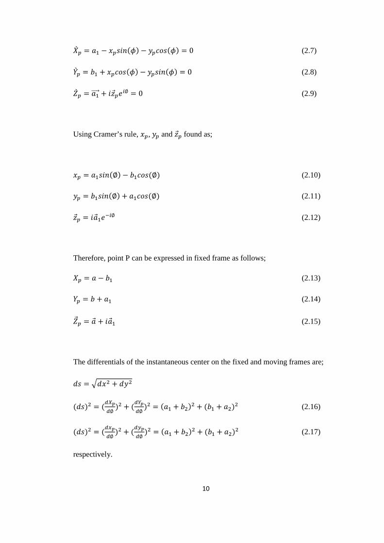
The differentials of the instantaneous center on the fixed and moving frames are;
𝑑𝑠 = �𝑑𝑥2 + 𝑑𝑦2
(𝑑𝑠)2 = (𝑑𝑋𝑝𝑑∅
)2 + (𝑑𝑌𝑝𝑑∅
)2 = (𝑎1 + 𝑏2)2 + (𝑏1 + 𝑎2)2 (2.16)
(𝑑𝑠)2 = (𝑑𝑥𝑝𝑑∅
)2 + (𝑑𝑦𝑝𝑑∅
)2 = (𝑎1 + 𝑏2)2 + (𝑏1 + 𝑎2)2 (2.17)
respectively.
11
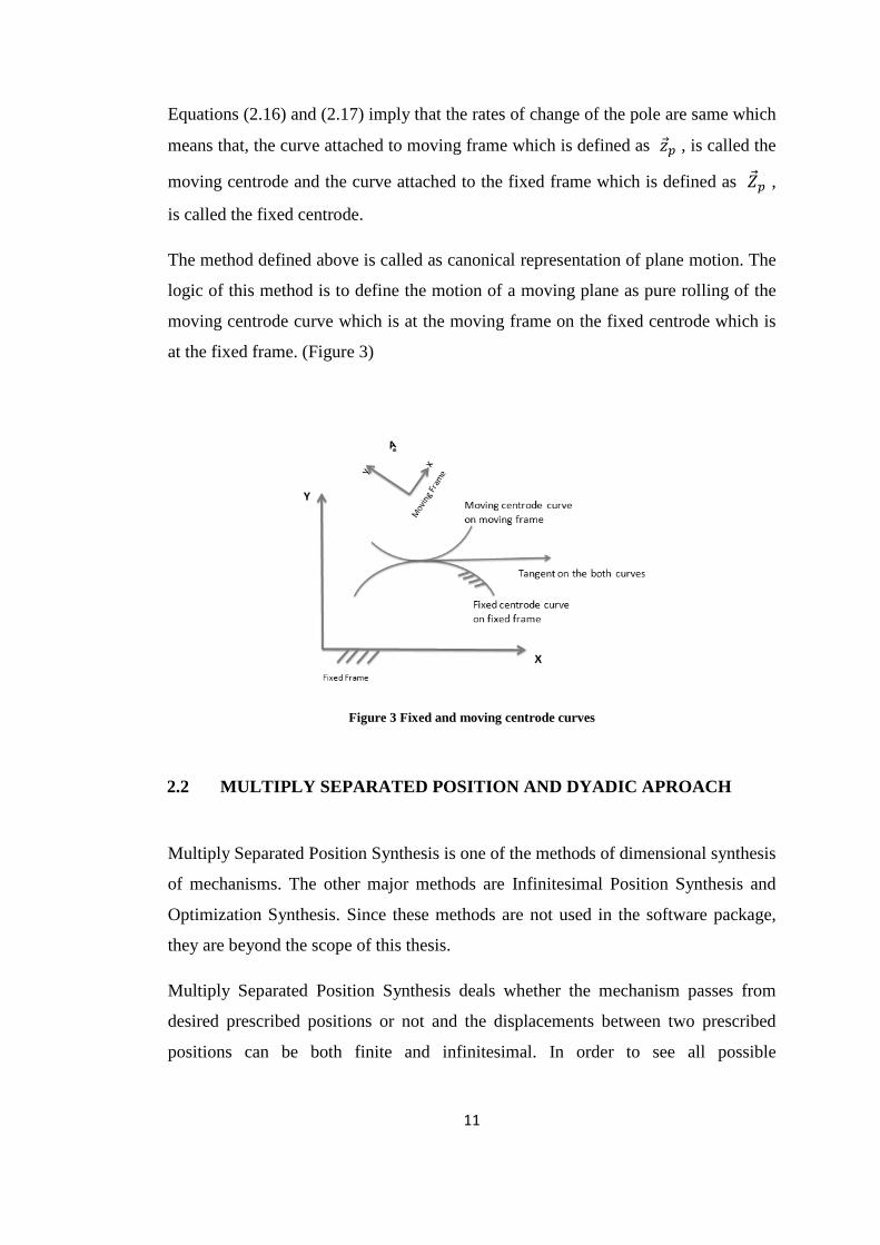
Equations (2.16) and (2.17) imply that the rates of change of the pole are same which
means that, the curve attached to moving frame which is defined as 𝑧𝑝 , is called the
moving centrode and the curve attached to the fixed frame which is defined as �⃗�𝑝 ,
is called the fixed centrode.
The method defined above is called as canonical representation of plane motion. The
logic of this method is to define the motion of a moving plane as pure rolling of the
moving centrode curve which is at the moving frame on the fixed centrode which is
at the fixed frame. (Figure 3)
Figure 3 Fixed and moving centrode curves
2.2 MULTIPLY SEPARATED POSITION AND DYADIC APROACH
Multiply Separated Position Synthesis is one of the methods of dimensional synthesis
of mechanisms. The other major methods are Infinitesimal Position Synthesis and
Optimization Synthesis. Since these methods are not used in the software package,
they are beyond the scope of this thesis.
Multiply Separated Position Synthesis deals whether the mechanism passes from
desired prescribed positions or not and the displacements between two prescribed
positions can be both finite and infinitesimal. In order to see all possible

12
combinations of finitely and infinitesimally separated positions, the basic notations
used are shown in Table 1 which is introduced by Tesar [33].
Table 1 Representation for finitely and infinitesimally separated positions
P-P Two finitely separated positions
PP Two infinitesimally separated
positions
Therefore, P-PP is used for three multiply separated positions and the infinitesimally
separated position belongs to the second finitely separated position.
In Multiply Separated Positions Synthesis, the mechanisms have to satisfy a finite
number of constraint equations at the prescribed points. In order to obtain those
constraint equations dyadic approach is used which introduced by Erdman [22].
In dyadic approach, the planar linkages are thought of as combinations of vector
pairs called dyads. For example, the four-bar mechanism shown in Figure 4 can be
perceived as two dyads. These dyads have to be solved separately and then have to
be combined in order to form a whole mechanism.
Figure 4 Dyadic representation of four-bar mechanism
13
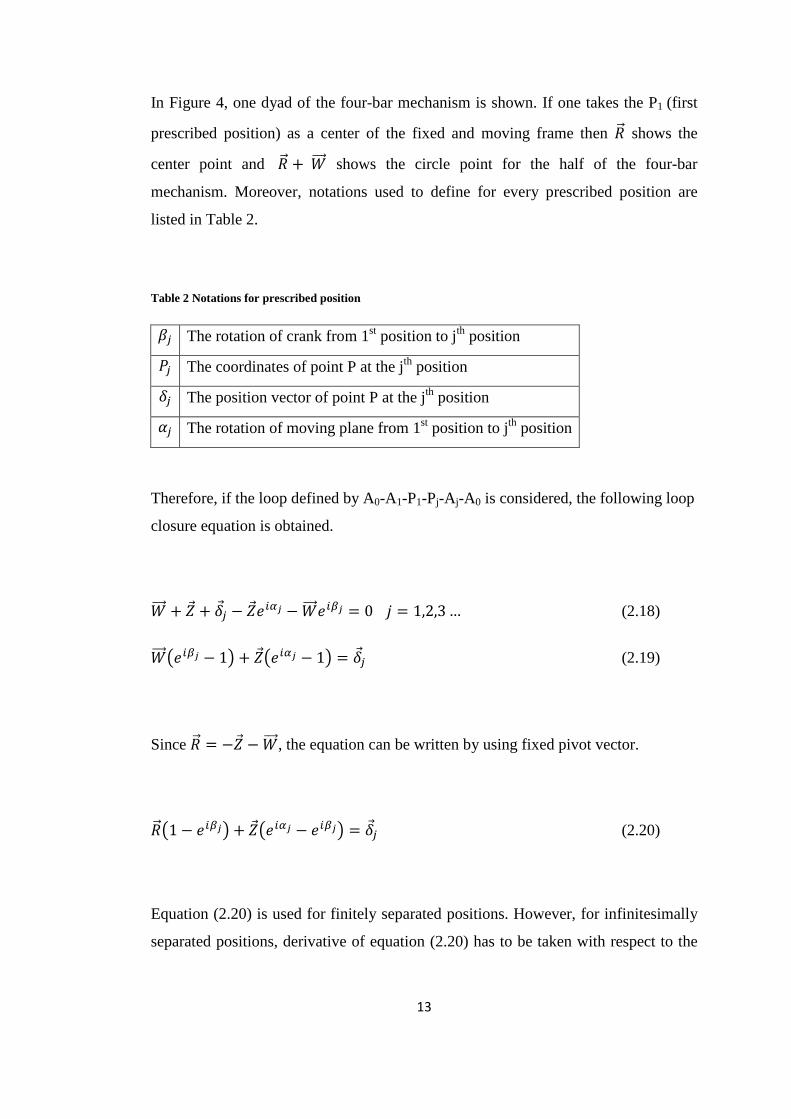
In Figure 4, one dyad of the four-bar mechanism is shown. If one takes the P1 (first
prescribed position) as a center of the fixed and moving frame then 𝑅�⃗ shows the
center point and 𝑅�⃗ + 𝑊���⃗ shows the circle point for the half of the four-bar
mechanism. Moreover, notations used to define for every prescribed position are
listed in Table 2.
Table 2 Notations for prescribed position
𝛽𝑗 The rotation of crank from 1st position to jth position
𝑃𝑗 The coordinates of point P at the jth position
𝛿𝑗 The position vector of point P at the jth position
𝛼𝑗 The rotation of moving plane from 1st position to jth position
Therefore, if the loop defined by A0-A1-P1-Pj-Aj-A0 is considered, the following loop
closure equation is obtained.
𝑊���⃗ + �⃗� + 𝛿𝑗 − �⃗�𝑒𝑖𝛼𝑗 −𝑊���⃗ 𝑒𝑖𝛽𝑗 = 0 𝑗 = 1,2,3 … (2.18)
𝑊���⃗ �𝑒𝑖𝛽𝑗 − 1� + �⃗��𝑒𝑖𝛼𝑗 − 1� = 𝛿𝑗 (2.19)
Since 𝑅�⃗ = −�⃗� −𝑊���⃗ , the equation can be written by using fixed pivot vector.
𝑅�⃗ �1 − 𝑒𝑖𝛽𝑗� + �⃗��𝑒𝑖𝛼𝑗 − 𝑒𝑖𝛽𝑗� = 𝛿𝑗 (2.20)
Equation (2.20) is used for finitely separated positions. However, for infinitesimally
separated positions, derivative of equation (2.20) has to be taken with respect to the

14
given angular displacement value. For motion generation synthesis, the loop closure
equation for infinitesimally separated positions is as follows;
𝑅�⃗ 𝑑𝑑𝛼�(1 − 𝑒𝑖𝛽)�
𝛽=𝛽𝑗+ �⃗� 𝑑
𝑑𝛼�(𝑒𝑖𝛼 − 𝑒𝑖𝛽)�𝛼=𝛼𝑗
𝛽=𝛽𝑗
= 𝑑𝑑𝛼�𝛿𝑗(𝛼)�
𝛼=𝛼𝑗 (2.21)
For situations where the finitely and infinitesimally separated positions are combined
following equation is used.
𝑅�⃗ 𝑑𝑘
𝑑𝛼𝑘�(1 − 𝑒𝑖𝛽)�
𝛽=𝛽𝑗+ �⃗� 𝑑𝑘
𝑑𝛼𝑘�(𝑒𝑖𝛼 − 𝑒𝑖𝛽)�𝛼=𝛼𝑗
𝛽=𝛽𝑗
= 𝑑𝑘
𝑑𝛼𝑘�𝛿𝑗(𝛼)�
𝛼=𝛼𝑗 (2.22)
where;
j: index of the finitely separated position
k: index of the infinitesimally separated position corresponding to a finitely separated
position
l: index of the total separated position
More compact form of equation (2.22) can be written as;
𝑅�⃗ (𝜎𝑙 − 𝑏𝑙) + �⃗�(𝑎𝑙 − 𝑏𝑙) = 𝛿𝑙 (2.23)
𝑤ℎ𝑒𝑟𝑒 𝑎𝑙 = � 𝑑𝑘
𝑑𝛼𝑘𝑒𝑖𝛼�
𝛼=𝜎𝑙𝛼𝑗
; 𝑏𝑙 = � 𝑑𝑘
𝑑𝛼𝑘𝑒𝑖𝛼�
𝛽=𝜎𝑙𝛽𝑗
; 𝛿𝑙 = � 𝑑𝑘
𝑑𝛼𝑘𝛿�
𝛿��⃗ =𝜎𝑙𝛿��⃗ 𝑗
𝜎𝑙𝑘 = 0 (𝑘 = 0,𝜎𝑙 = 1 𝑜𝑟 𝑘 ≠ 0, 𝜎𝑙 = 0)
In Multiply Separated Position Synthesis, there are mainly three different tasks for
mechanism synthesis. They are namely; motion, path and function generation.
According to those tasks, the unknowns and prescribed positions can be changed.
15
2.3 SYNTHESIS TASKS
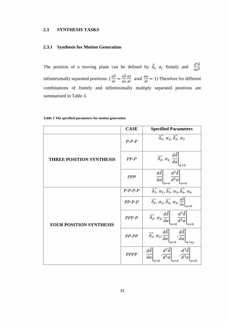
2.3.1 Synthesis for Motion Generation
The position of a moving plane can be defined by 𝛿𝑗 , 𝛼𝑗 finitely and 𝑑𝑘𝛿��⃗
𝑑𝛼𝑘
infinitesimally separated positions. ( 𝑑𝛿��⃗
𝑑𝑡= 𝑑𝛿��⃗
𝑑𝛼𝑑𝛼𝑑𝑡
𝑎𝑛𝑑 𝑑𝛼𝑑𝑡
= 1) Therefore for different
combinations of finitely and infinitesimally multiply separated positions are
summarized in Table 3.
Table 3 The specified parameters for motion generation
CASE Specified Parameters
THREE POSITION SYNTHESIS
P-P-P 𝛿2����⃗ , 𝛼2, 𝛿3����⃗ , 𝛼3
PP-P 𝛿2����⃗ , 𝛼2, �𝑑𝛿𝑑𝛼�𝛼=0
PPP �𝑑𝛿𝑑𝛼�𝛼=0
�𝑑2𝛿
𝑑2𝛼�𝛼=0
FOUR POSITION SYNTHESIS
P-P-P-P 𝛿2����⃗ , 𝛼2, 𝛿3����⃗ , 𝛼3, 𝛿4����⃗ , 𝛼4
PP-P-P 𝛿2����⃗ , 𝛼2, 𝛿3����⃗ , 𝛼3, �𝑑𝛿��⃗
𝑑𝛼�𝛼=0
PPP-P 𝛿2����⃗ , 𝛼2, �𝑑𝛿𝑑𝛼�𝛼=0
�𝑑2𝛿
𝑑2𝛼�𝛼=0
PP-PP 𝛿2����⃗ , 𝛼2, �𝑑𝛿𝑑𝛼�𝛼=0
, �𝑑𝛿𝑑𝛼�𝛼=𝛼2
PPPP �𝑑𝛿𝑑𝛼�𝛼=0
, �𝑑2𝛿𝑑2𝛼
�𝛼=0
, �𝑑3𝛿𝑑3𝛼
�𝛼=0
16
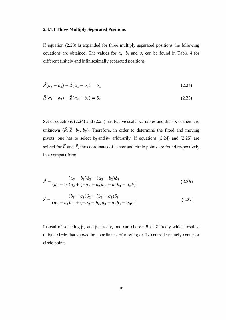
2.3.1.1 Three Multiply Separated Positions
If equation (2.23) is expanded for three multiply separated positions the following
equations are obtained. The values for 𝛼𝑖, 𝑏𝑖 and 𝜎𝑖 can be found in Table 4 for
different finitely and infinitesimally separated positions.
𝑅�⃗ (𝜎2 − 𝑏2) + �⃗�(𝑎2 − 𝑏2) = 𝛿2 (2.24)
𝑅�⃗ (𝜎3 − 𝑏3) + �⃗�(𝑎3 − 𝑏3) = 𝛿3 (2.25)
Set of equations (2.24) and (2.25) has twelve scalar variables and the six of them are
unknown (𝑅�⃗ , 𝑍���⃗ , 𝑏2, 𝑏3). Therefore, in order to determine the fixed and moving
pivots; one has to select 𝑏2 and 𝑏3 arbitrarily. If equations (2.24) and (2.25) are
solved for 𝑅�⃗ and �⃗�, the coordinates of center and circle points are found respectively
in a compact form.
𝑅�⃗ =(𝛼3 − 𝑏3)𝛿2 − (𝛼2 − 𝑏2)𝛿3
(𝛼3 − 𝑏3)𝜎2 + (−𝛼2 + 𝑏2)𝜎3 + 𝛼2𝑏3 − 𝛼3𝑏2 (2.26)
�⃗� =(𝑏3 − 𝜎3)𝛿2 − (𝑏2 − 𝜎2)𝛿3
(𝛼3 − 𝑏3)𝜎2 + (−𝛼2 + 𝑏2)𝜎3 + 𝛼2𝑏3 − 𝛼3𝑏2 (2.27)
Instead of selecting β2 and β3 freely, one can choose 𝑅�⃗ or �⃗� freely which result a
unique circle that shows the coordinates of moving or fix centrode namely center or
circle points.

17
Table 4 Explicit terms used in the dyad loop equation for three positions
CASE 𝜎2 𝜎3 𝛼2 𝛼3 𝑏2 𝑏3 𝛿2 𝛿3 Selected
Parameters
P-P-P 1 1 𝑒𝑖𝛼2 𝑒𝑖𝛼3 𝑒𝑖𝑏2 𝑒𝑖𝑏3 𝛿2����⃗ 𝛿3����⃗ 𝛽2 𝛽3
PP-P 0 1 i 𝑒𝑖𝛼2 𝑖�̇� 𝑒𝑖𝑏2 𝑑𝛿𝑑𝛼
𝛿2����⃗ �̇� 𝛽3
PPP 0 0 i -1 𝑖�̇� −�̇�2 + 𝑖�̈� 𝑑𝛿𝑑𝛼
𝑑2𝛿𝑑𝛼2
�̇� �̈�
In order to specify the locations of center points 𝑅�⃗ has to be specified. Therefore, the
dyad loop closure equation can be rewritten as;
�⃗� + 𝑊���⃗ = −𝑅�⃗ (2.28)
𝑎2�⃗� + 𝑏2𝑊���⃗ = 𝛿2 − 𝜎2𝑅�⃗ (2.29)
𝑎3�⃗� + 𝑏3𝑊���⃗ = 𝛿3 − 𝜎3𝑅�⃗ (2.30)
This set of equation can be solved for 𝑊���⃗ and �⃗� if the determinant of the coefficient
matrix is zero.
�1 1 −𝑅�⃗𝑏2 𝑎2 𝛿2 − 𝜎2𝑅�⃗
𝑏3 𝑎3 𝛿3 − 𝜎3𝑅�⃗� = 0
by expanding the matrix about the first column;
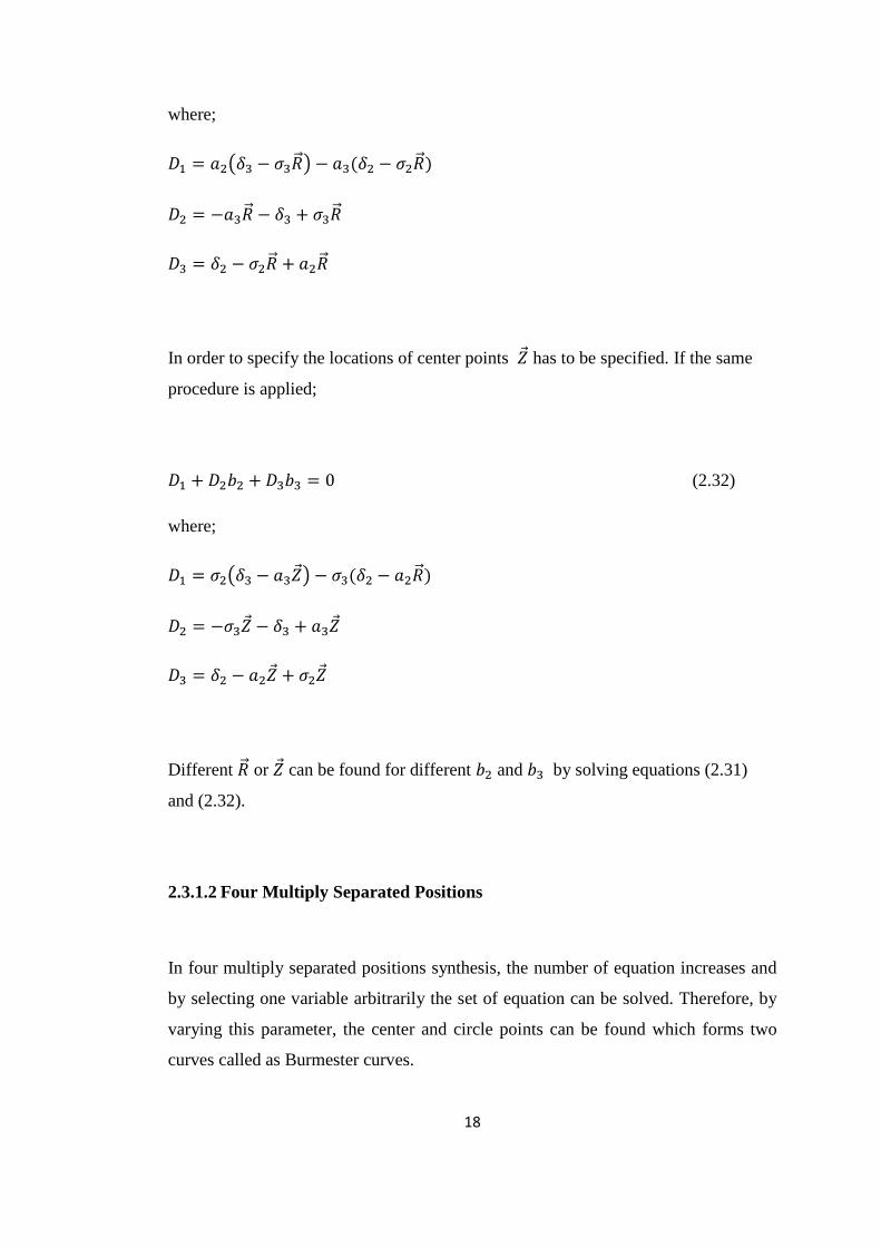
𝐷1 + 𝐷2𝑏2 + 𝐷3𝑏3 = 0 (2.31)
18
where;
𝐷1 = 𝑎2�𝛿3 − 𝜎3𝑅�⃗ � − 𝑎3(𝛿2 − 𝜎2𝑅�⃗ )
𝐷2 = −𝑎3𝑅�⃗ − 𝛿3 + 𝜎3𝑅�⃗
𝐷3 = 𝛿2 − 𝜎2𝑅�⃗ + 𝑎2𝑅�⃗
In order to specify the locations of center points �⃗� has to be specified. If the same
procedure is applied;
𝐷1 + 𝐷2𝑏2 + 𝐷3𝑏3 = 0 (2.32)
where;
𝐷1 = 𝜎2�𝛿3 − 𝑎3�⃗�� − 𝜎3(𝛿2 − 𝑎2𝑅�⃗ )
𝐷2 = −𝜎3�⃗� − 𝛿3 + 𝑎3�⃗�
𝐷3 = 𝛿2 − 𝑎2�⃗� + 𝜎2�⃗�
Different 𝑅�⃗ or �⃗� can be found for different 𝑏2 and 𝑏3 by solving equations (2.31)
and (2.32).
2.3.1.2 Four Multiply Separated Positions
In four multiply separated positions synthesis, the number of equation increases and
by selecting one variable arbitrarily the set of equation can be solved. Therefore, by
varying this parameter, the center and circle points can be found which forms two
curves called as Burmester curves.

19
As an example, the solution procedure of finitely separated position (P-P-P-P)
synthesis will be given. By equation (2.23) the following set of equation is obtained.
�1 − 𝑒𝑖𝛽2�𝑅�⃗ + �𝑒𝑖𝛼2 − 𝑒𝑖𝛽2��⃗� = 𝛿2 (2.33)
�1 − 𝑒𝑖𝛽3�𝑅�⃗ + �𝑒𝑖𝛼3 − 𝑒𝑖𝛽3��⃗� = 𝛿3 (2.34)
�1 − 𝑒𝑖𝛽4�𝑅�⃗ + �𝑒𝑖𝛼4 − 𝑒𝑖𝛽4��⃗� = 𝛿4 (2.35)
In order to solve the set of equation, 𝛽2, 𝛽3 or 𝛽4 is selected arbitrarily and every
selection will yield the same curves. The determinant of the augmented matrix of the
set of equation for selection of 𝛽2 arbitrarily will be;
�1 − 𝑒𝑖𝛽2 𝑒𝑖𝛼2 − 𝑒𝑖𝛽2 𝛿2����⃗ 1 − 𝑒𝑖𝛽3 𝑒𝑖𝛼3 − 𝑒𝑖𝛽3 𝛿3����⃗
1 − 𝑒𝑖𝛽4 𝑒𝑖𝛼4 − 𝑒𝑖𝛽4 𝛿4����⃗� = 0
𝐷1 + 𝐷2𝑒𝑖𝛽3 + 𝐷3𝑒𝑖𝛽4 = 0 (2.36)
where;
𝐷1 = �1 − 𝑒𝑖𝛽2��𝛿4����⃗ 𝑒𝑖𝛼3 − 𝛿3����⃗ 𝑒𝑖𝛼4� + 𝛿2����⃗ �𝑒𝑖𝛼4 − 𝑒𝑖𝛼3� + 𝛿3����⃗ �𝑒𝑖𝛼2 − 𝑒𝑖𝛽2�
+ 𝛿4����⃗ (𝑒𝑖𝛽2 − 𝑒𝑖𝛼2)
𝐷2 = 𝛿2����⃗ �1 − 𝑒𝑖𝛼4� − 𝛿4����⃗ (1 − 𝑒𝑖𝛼2)
𝐷3 = 𝛿2����⃗ �𝑒𝑖𝛼3 − 1� − 𝛿3����⃗ (𝑒𝑖𝛼2 − 1)
20
2.3.2 Synthesis for Path Generation
In path generation task, the points on the coupler path are correlated with the input
link positions. The synthesis procedure of path generation is same as motion
generation. However, at this time, crank rotations (𝛽𝑗) are known, but, coupler
rotations (𝛼𝑗) are not known. Therefore, the motion generation calculation routines
can be used if 𝛽𝑗 values are entered as if they were 𝛼𝑗. As a result, the first dyad can
be constructed. Since the coupler rotations are found, the crank rotations in the
second dyad are found by the same routines of motion generation synthesis.
2.3.3 Synthesis for Function Generation
In function generation task, the prescribed rotations of the input link are correlated
with the output link. Since the rotations of input links are given, the dyad containing
the input link is known. The other dyad which contains the output link can be found
by the path generation synthesis procedure.
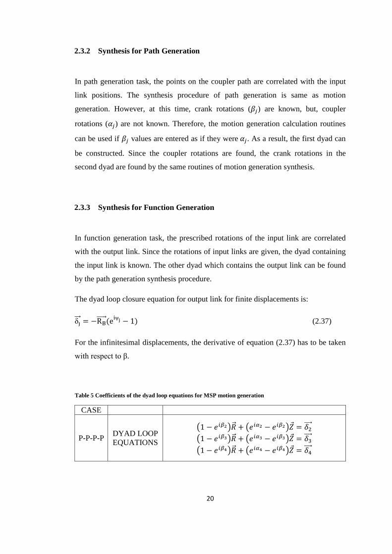
The dyad loop closure equation for output link for finite displacements is:
δȷ��⃗ = −RB�����⃗ (eiψj − 1) (2.37)
For the infinitesimal displacements, the derivative of equation (2.37) has to be taken
with respect to β.
Table 5 Coefficients of the dyad loop equations for MSP motion generation
CASE
P-P-P-P DYAD LOOP EQUATIONS
�1 − 𝑒𝑖𝛽2�𝑅�⃗ + �𝑒𝑖𝛼2 − 𝑒𝑖𝛽2��⃗� = 𝛿2����⃗ �1 − 𝑒𝑖𝛽3�𝑅�⃗ + �𝑒𝑖𝛼3 − 𝑒𝑖𝛽3��⃗� = 𝛿3����⃗ �1 − 𝑒𝑖𝛽4�𝑅�⃗ + �𝑒𝑖𝛼4 − 𝑒𝑖𝛽4��⃗� = 𝛿4����⃗
21
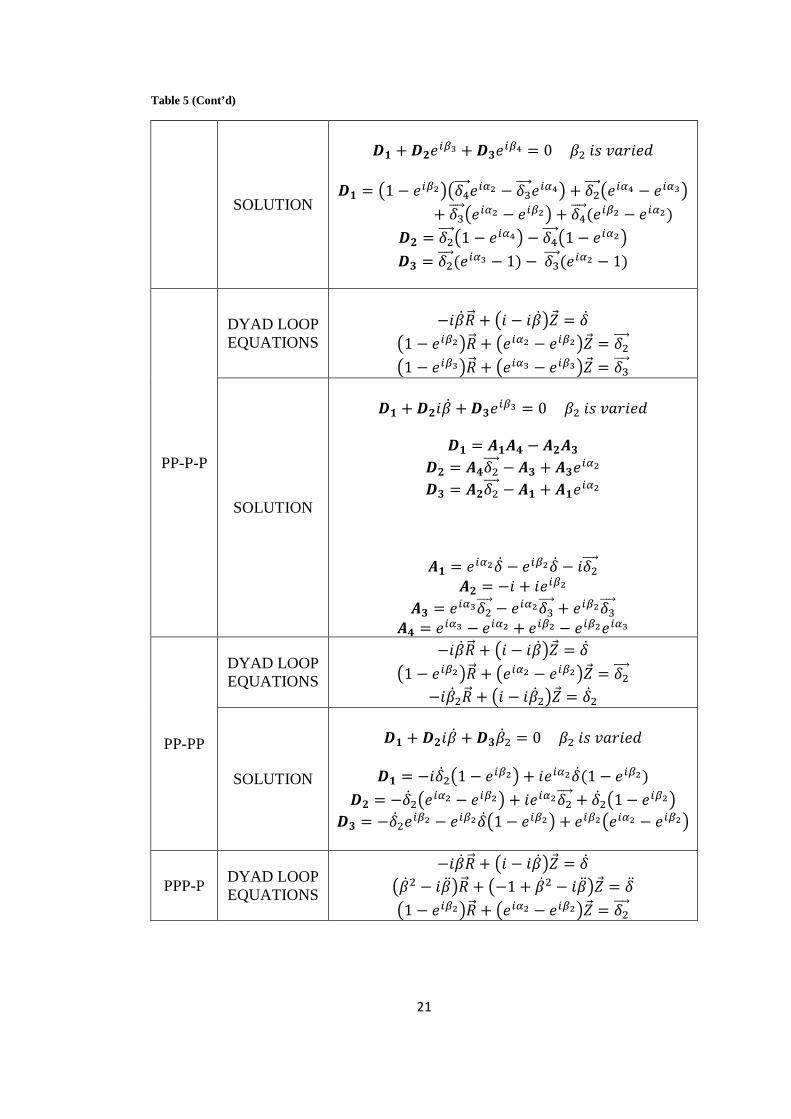
Table 5 (Cont’d)
SOLUTION
𝑫𝟏 + 𝑫𝟐𝑒𝑖𝛽3 + 𝑫𝟑𝑒𝑖𝛽4 = 0 𝛽2 𝑖𝑠 𝑣𝑎𝑟𝑖𝑒𝑑
𝑫𝟏 = �1 − 𝑒𝑖𝛽2��𝛿4����⃗ 𝑒𝑖𝛼2 − 𝛿3����⃗ 𝑒𝑖𝛼4� + 𝛿2����⃗ �𝑒𝑖𝛼4 − 𝑒𝑖𝛼3�
+ 𝛿3����⃗ �𝑒𝑖𝛼2 − 𝑒𝑖𝛽2� + 𝛿4����⃗ (𝑒𝑖𝛽2 − 𝑒𝑖𝛼2) 𝑫𝟐 = 𝛿2����⃗ �1 − 𝑒𝑖𝛼4� − 𝛿4����⃗ �1 − 𝑒𝑖𝛼2� 𝑫𝟑 = 𝛿2����⃗ (𝑒𝑖𝛼3 − 1) − 𝛿3����⃗ (𝑒𝑖𝛼2 − 1)
PP-P-P
DYAD LOOP EQUATIONS
−𝑖�̇�𝑅�⃗ + �𝑖 − 𝑖�̇���⃗� = �̇�
�1 − 𝑒𝑖𝛽2�𝑅�⃗ + �𝑒𝑖𝛼2 − 𝑒𝑖𝛽2��⃗� = 𝛿2����⃗ �1 − 𝑒𝑖𝛽3�𝑅�⃗ + �𝑒𝑖𝛼3 − 𝑒𝑖𝛽3��⃗� = 𝛿3����⃗
SOLUTION
𝑫𝟏 + 𝑫𝟐𝑖�̇� + 𝑫𝟑𝑒𝑖𝛽3 = 0 𝛽2 𝑖𝑠 𝑣𝑎𝑟𝑖𝑒𝑑
𝑫𝟏 = 𝑨𝟏𝑨𝟒 − 𝑨𝟐𝑨𝟑
𝑫𝟐 = 𝑨𝟒𝛿2����⃗ − 𝑨𝟑 + 𝑨𝟑𝑒𝑖𝛼2 𝑫𝟑 = 𝑨𝟐𝛿2����⃗ − 𝑨𝟏 + 𝑨𝟏𝑒𝑖𝛼2
𝑨𝟏 = 𝑒𝑖𝛼2�̇� − 𝑒𝑖𝛽2�̇� − 𝑖𝛿2����⃗ 𝑨𝟐 = −𝑖 + 𝑖𝑒𝑖𝛽2
𝑨𝟑 = 𝑒𝑖𝛼3𝛿2����⃗ − 𝑒𝑖𝛼2𝛿3����⃗ + 𝑒𝑖𝛽2𝛿3����⃗ 𝑨𝟒 = 𝑒𝑖𝛼3 − 𝑒𝑖𝛼2 + 𝑒𝑖𝛽2 − 𝑒𝑖𝛽2𝑒𝑖𝛼3
PP-PP
DYAD LOOP EQUATIONS
−𝑖�̇�𝑅�⃗ + �𝑖 − 𝑖�̇���⃗� = �̇� �1 − 𝑒𝑖𝛽2�𝑅�⃗ + �𝑒𝑖𝛼2 − 𝑒𝑖𝛽2��⃗� = 𝛿2����⃗
−𝑖�̇�2𝑅�⃗ + �𝑖 − 𝑖�̇�2��⃗� = �̇�2
SOLUTION
𝑫𝟏 + 𝑫𝟐𝑖�̇� + 𝑫𝟑�̇�2 = 0 𝛽2 𝑖𝑠 𝑣𝑎𝑟𝑖𝑒𝑑
𝑫𝟏 = −𝑖�̇�2�1 − 𝑒𝑖𝛽2� + 𝑖𝑒𝑖𝛼2�̇�(1 − 𝑒𝑖𝛽2)
𝑫𝟐 = −�̇�2�𝑒𝑖𝛼2 − 𝑒𝑖𝛽2� + 𝑖𝑒𝑖𝛼2𝛿2����⃗ + �̇�2�1 − 𝑒𝑖𝛽2� 𝑫𝟑 = −�̇�2𝑒𝑖𝛽2 − 𝑒𝑖𝛽2�̇��1− 𝑒𝑖𝛽2� + 𝑒𝑖𝛽2�𝑒𝑖𝛼2 − 𝑒𝑖𝛽2�
PPP-P DYAD LOOP EQUATIONS
−𝑖�̇�𝑅�⃗ + �𝑖 − 𝑖�̇���⃗� = �̇� ��̇�2 − 𝑖�̈��𝑅�⃗ + �−1 + �̇�2 − 𝑖�̈���⃗� = �̈� �1 − 𝑒𝑖𝛽2�𝑅�⃗ + �𝑒𝑖𝛼2 − 𝑒𝑖𝛽2��⃗� = 𝛿2����⃗

22
Table 5 (Cont’d)
SOLUTION
𝑫𝟏 + 𝑫𝟐𝑖�̇� + 𝑫𝟑(−�̇�2 + 𝑖�̈�) = 0 𝛽2 𝑖𝑠 𝑣𝑎𝑟𝑖𝑒𝑑
𝑫𝟏 = 𝑖�̈��1 − 𝑒𝑖𝛽2� + �̇��1 − 𝑒𝑖𝛽2�
𝑫𝟐 = 𝛿2����⃗ + �̈��𝑒𝑖𝛼2 − 1� 𝑫𝟐 = 𝑖𝛿2����⃗ + �̇��1 − 𝑒𝑖𝛼2�
PPPP
DYAD LOOP EQUATIONS
−𝑖�̇�𝑅�⃗ + �𝑖 − 𝑖�̇���⃗� = �̇� ��̇�2 − 𝑖�̈��𝑅�⃗ + �−1 + �̇�2 − 𝑖�̈���⃗� = �̈�
�3�̇��̈� − 𝑖𝛽 + 𝑖�̇�3�𝑅�⃗ + �−𝑖 + 3�̇��̈� − 𝑖𝛽 + +𝑖�̇�3��⃗�= 𝛿
SOLUTION
𝑫𝟏 + 𝑫𝟐�̈� + 𝑫𝟑𝛽 = 0 𝛽2 𝑖𝑠 𝑣𝑎𝑟𝑖𝑒𝑑
𝑫𝟏 = (−𝑖𝛿 − �̈� + 𝑖��̇� + 𝛿��̇� + (�̈� − 𝑖�̇�)�̇�2)�̇�
𝑫𝟐 = �̇� + 𝛿 + �̇�(−3�̇� − 3𝑖�̈�) 𝑫𝟑 = −�̈� + 𝑖�̇�
2.4 DEFECTS IN MECHANISM SYNTHESIS
When the points on the Burmester curve are used to construct mechanism they may
not fulfill the prescribed geometrical conditions, although it satisfies the conditions
theoretically. This occurs due to branch and circuit defects, order problem and
Grashof condition.
In branch defect, the mechanism has to be disassembled from a joint and then
assembled again in order to obtain prescribed positions. Circuit defect occurs when
the prescribed positions are not in the same disjointed range of motion of input link.
Order problem occurs since orders of prescribed positions cannot be considered in
synthesis procedures. Therefore, the mechanism selected from Burmester curve, may
not pass in desired order. Moreover, the obtained mechanism may be double rocker,
23
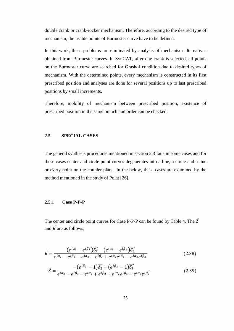
double crank or crank-rocker mechanism. Therefore, according to the desired type of
mechanism, the usable points of Burmester curve have to be defined.
In this work, these problems are eliminated by analysis of mechanism alternatives
obtained from Burmester curves. In SynCAT, after one crank is selected, all points
on the Burmester curve are searched for Grashof condition due to desired types of
mechanism. With the determined points, every mechanism is constructed in its first
prescribed position and analyses are done for several positions up to last prescribed
positions by small increments.
Therefore, mobility of mechanism between prescribed position, existence of
prescribed position in the same branch and order can be checked.
2.5 SPECIAL CASES
The general synthesis procedures mentioned in section 2.3 fails in some cases and for
these cases center and circle point curves degenerates into a line, a circle and a line
or every point on the coupler plane. In the below, these cases are examined by the
method mentioned in the study of Polat [26].
2.5.1 Case P-P-P
The center and circle point curves for Case P-P-P can be found by Table 4. The �⃗� and 𝑅�⃗ are as follows;
𝑅�⃗ =�𝑒𝑖𝛼3 − 𝑒𝑖𝛽3 �𝛿2����⃗ − �𝑒𝑖𝛼2 − 𝑒𝑖𝛽2 �𝛿3����⃗
𝑒𝑖𝛼3 − 𝑒𝑖𝛽3 − 𝑒𝑖𝛼2 + 𝑒𝑖𝛽2 + 𝑒𝑖𝛼2𝑒𝑖𝛽3 − 𝑒𝑖𝛼3𝑒𝑖𝛽2 (2.38)
−�⃗� =−�𝑒𝑖𝛽3 − 1�𝛿2����⃗ + �𝑒𝑖𝛽2 − 1�𝛿3����⃗
𝑒𝑖𝛼3 − 𝑒𝑖𝛽3 − 𝑒𝑖𝛼2 + 𝑒𝑖𝛽2 + 𝑒𝑖𝛼2𝑒𝑖𝛽3 − 𝑒𝑖𝛼3𝑒𝑖𝛽2 (2.39)

24
If the prescribed all positions are parallel (i.e. 𝛼2=𝛼3 = 0), �⃗� and 𝑅�⃗ becomes as follows;
𝑅�⃗ =�1 − 𝑒𝑖𝛽3 �𝛿2����⃗ − �1 − 𝑒𝑖𝛽2 �𝛿3����⃗
0 (2.40)
−�⃗� =−�𝑒𝑖𝛽3 − 1�𝛿2����⃗ + �𝑒𝑖𝛽2 − 1�𝛿3����⃗
0 (2.41)
The equations above have a solution if the numerators are zero.
−�𝑒𝑖𝛽3 − 1�𝛿2����⃗ + �𝑒𝑖𝛽2 − 1�𝛿3����⃗ = 0 (2.42)
In the equation, if 𝛿3����⃗
𝛿2����⃗ is pure real then the crank rotations (i.e. β2 = β3 = 0) have to
be zero and if δ3����⃗
δ2����⃗ is not pure real, the crank rotations are fixed and can be obtained
from above equation. In both cases, the every point of the moving plane can be
selected as a circle point. The other configurations for special cases are shown in
table below.
Table 6 Special cases for P-P-P
Condition Circle Point Center Point
𝛼2 = 𝛼3= 0
𝛿3����⃗
𝛿2����⃗ is real At infinity Every point
𝛿3����⃗
𝛿2����⃗ is not real Every point Every point
𝛼2 = 0,𝛼3 ≠ 0 Line Line
𝛼2 ≠ 0,𝛼3 = 0 Line Line
𝛼2 = 𝛼3 ≠ 0 Line Line
25
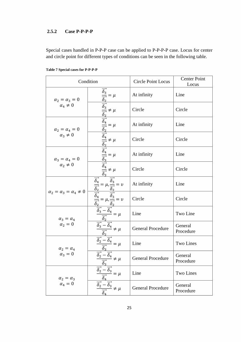
2.5.2 Case P-P-P-P
Special cases handled in P-P-P case can be applied to P-P-P-P case. Locus for center and circle point for different types of conditions can be seen in the following table.
Table 7 Special cases for P-P-P-P
Condition Circle Point Locus Center Point Locus
𝛼2 = 𝛼3 = 0 𝛼4 ≠ 0
𝛿3����⃗
𝛿2����⃗= 𝜇 At infinity Line
𝛿3����⃗
𝛿2����⃗≠ 𝜇 Circle Circle
𝛼2 = 𝛼4 = 0 𝛼3 ≠ 0
𝛿4����⃗
𝛿2����⃗= 𝜇 At infinity Line
𝛿4����⃗
𝛿2����⃗≠ 𝜇 Circle Circle
𝛼3 = 𝛼4 = 0 𝛼2 ≠ 0
𝛿4����⃗
𝛿3����⃗= 𝜇 At infinity Line
𝛿4����⃗
𝛿3����⃗≠ 𝜇 Circle Circle
𝛼2 = 𝛼3 = 𝛼4 ≠ 0
𝛿4����⃗
𝛿2����⃗= 𝜇,
𝛿3����⃗
𝛿2����⃗= 𝜐 At infinity Line
𝛿4����⃗
𝛿2����⃗= 𝜇,
𝛿3����⃗
𝛿2����⃗= 𝜐 Circle Circle
𝛼3 = 𝛼4 𝛼2 = 0
𝛿3����⃗ − 𝛿4����⃗
𝛿2����⃗= 𝜇 Line Two Line
𝛿3����⃗ − 𝛿4����⃗
𝛿2����⃗≠ 𝜇 General Procedure General
Procedure
𝛼2 = 𝛼4 𝛼3 = 0
𝛿2����⃗ − 𝛿4����⃗
𝛿3����⃗= 𝜇 Line Two Lines
𝛿2����⃗ − 𝛿4����⃗
𝛿3����⃗≠ 𝜇 General Procedure General
Procedure
𝛼2 = 𝛼3 𝛼4 = 0
𝛿2����⃗ − 𝛿3����⃗
𝛿4����⃗= 𝜇 Line Two Lines
𝛿2����⃗ − 𝛿3����⃗
𝛿4����⃗≠ 𝜇 General Procedure General
Procedure

26
2.5.3 Case PP-P-P
Special case in PP-P-P occurs when the coupler rotations are same. The following table shows the locus equations for different types of conditions.
Table 8 Special cases for PP-P-P
Condition Circle Point Locus Center Point Locus
𝛼2 = 0 𝛼3 = 0
𝛿3����⃗
𝛿2����⃗ is
real At infinity −�⃗� = −𝑖𝛿2����⃗ −
�𝑒𝑖𝛽2 − 1�𝑖𝛽
𝛿3����⃗
𝛿3����⃗
𝛿2����⃗ is
not real
Line
𝑅�⃗ =�1 − 𝑒𝑖𝛽2 �𝛿2����⃗ − �𝑖 − 𝑖�̇��𝛿3����⃗
𝑖(𝑒𝑖𝛽2 − 1)
Line
−�⃗� =−�𝑒𝑖𝛽2 − 1�𝛿2����⃗ − 𝑖�̇�𝛿3����⃗
𝑖(𝑒𝑖𝛽2 − 1)
2.5.4 Case PPPP
The equation of synthesis of PPPP generation and the coefficients are as follows;
𝑫𝟏 + 𝑫𝟐�̈� + 𝑫𝟑𝛽 = 0
𝑫𝟏 = (−𝑖𝛿 − �̈� + 𝑖��̇� + 𝛿��̇� + (�̈� − 𝑖�̇�)�̇�2)�̇� (2.43)
𝑫𝟐 = �̇� + 𝛿 + �̇�(−3�̇� − 3𝑖�̈�)
𝑫𝟑 = −�̈� + 𝑖�̇�
The general solution procedure fails when �̇�, 𝛿 are real and �̈� is imaginary or vice
versa. In such a cases 𝑫𝟏, 𝑫𝟑 are real and 𝑫𝟐 is imaginary or vice versa respectively.
In these cases, the equations can be satisfied only if 𝑫𝟐 = 0 or �̈� = 0.
If 𝑫𝟐 = 0 is solved for �̇�, then �̇� is;
�̇� =�̇� + 𝛿
3(�̇� + 𝑖�̈�) (2.44)
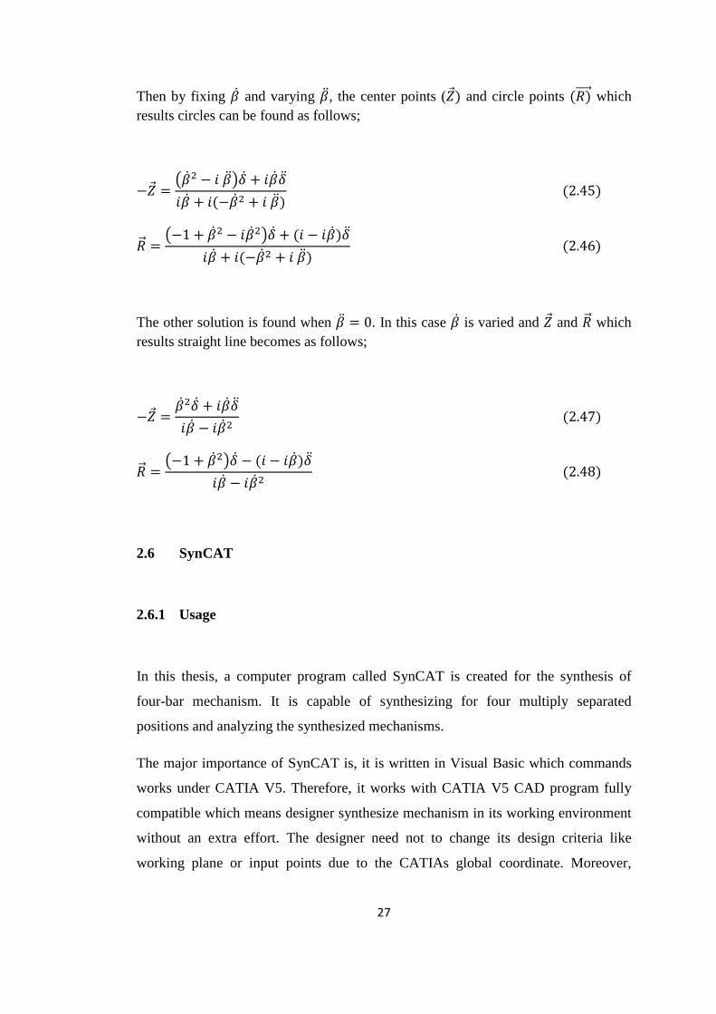
27
Then by fixing �̇� and varying �̈�, the center points (�⃗�) and circle points (𝑅)����⃗ which results circles can be found as follows;
−�⃗� =��̇�2 − 𝑖 �̈���̇� + 𝑖�̇��̈�𝑖�̇� + 𝑖(−�̇�2 + 𝑖 �̈�)
(2.45)
𝑅�⃗ =�−1 + �̇�2 − 𝑖�̇�2��̇� + (𝑖 − 𝑖�̇�)�̈�
𝑖�̇� + 𝑖(−�̇�2 + 𝑖 �̈�) (2.46)
The other solution is found when �̈� = 0. In this case �̇� is varied and �⃗� and 𝑅�⃗ which results straight line becomes as follows;
−�⃗� =�̇�2�̇� + 𝑖�̇��̈�𝑖�̇� − 𝑖�̇�2
(2.47)
𝑅�⃗ =�−1 + �̇�2��̇� − (𝑖 − 𝑖�̇�)�̈�
𝑖�̇� − 𝑖�̇�2 (2.48)
2.6 SynCAT
2.6.1 Usage
In this thesis, a computer program called SynCAT is created for the synthesis of
four-bar mechanism. It is capable of synthesizing for four multiply separated
positions and analyzing the synthesized mechanisms.
The major importance of SynCAT is, it is written in Visual Basic which commands
works under CATIA V5. Therefore, it works with CATIA V5 CAD program fully
compatible which means designer synthesize mechanism in its working environment
without an extra effort. The designer need not to change its design criteria like
working plane or input points due to the CATIAs global coordinate. Moreover,

28
during creation of SynCAT, the needs of Aerospace Industry are taken into account.
Since space allocation is very limited in such industries, selection of interested
regions can be used in SynCAT. Also in order to increase the possibilities, SynCAT
is capable of modifying the input variables.
SynCAT consists three different synthesis types namely path, function and motion
generation. For every synthesis type there are five different variations for four
multiply separated position synthesis which are P-P-P-P, PP-P-P, PP-PP, PPP-P and
PPPP. In order to show usage of SynCAT, function generation for PP-P-P will be
shown as an example.
Figure 5 SynCAT synthesis generation types
Figure 6 SynCAT function generation MSP types
29
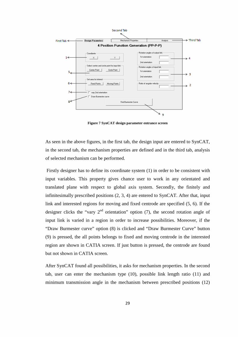
Figure 7 SynCAT design parameter entrance screen
As seen in the above figures, in the first tab, the design input are entered to SynCAT,
in the second tab, the mechanism properties are defined and in the third tab, analysis
of selected mechanism can be performed.
Firstly designer has to define its coordinate system (1) in order to be consistent with
input variables. This property gives chance user to work in any orientated and
translated plane with respect to global axis system. Secondly, the finitely and
infinitesimally prescribed positions (2, 3, 4) are entered to SynCAT. After that, input
link and interested regions for moving and fixed centrode are specified (5, 6). If the
designer clicks the “vary 2nd orientation” option (7), the second rotation angle of
input link is varied in a region in order to increase possibilities. Moreover, if the
“Draw Burmester curve” option (8) is clicked and “Draw Burmester Curve” button
(9) is pressed, the all points belongs to fixed and moving centrode in the interested
region are shown in CATIA screen. If just button is pressed, the centrode are found
but not shown in CATIA screen.
After SynCAT found all possibilities, it asks for mechanism properties. In the second
tab, user can enter the mechanism type (10), possible link length ratio (11) and
minimum transmission angle in the mechanism between prescribed positions (12)

30
and by pressing “Search for suitable mechanism” the all possible output cranks are
shown in CATIA screen. Moreover, in Third Tab, selected suitable mechanisms can
be analyzed for its kinematic properties.
The all output reflected to CATIA can be seen in figure below.
Figure 8 SynCAT mechanism properties entrance screen
Figure 9 View of SynCAT output in CATIA screen

31
2.6.2 Interface between CATIA and SynCAT
Communication between CATIA and SynCAT starts by selecting points for desired
positions and region of interests. In this step, coordinates of points (X, Y, Z) with
respect to CATIAs global coordinates are stored in SynCAT by visual basic code
given in Appendix B.
Nevertheless, in order to use the stored points in Burmester theory, they have to be
transformed into a new coordinate system (x, y, z) such that all points lie on the –xy
plane. After transformation, Burmester curves can be found by easily by Burmester
theory. However, points at Burmester curves have to be transformed into CATIAs
global coordinate before printing them onto CATIA.
Moreover, printing points at Burmester curve and suitable cranks onto CATIA are
done by visual basic code given in Appendix C and D.

32
CHAPTER 3
3. MECHANISM SYNTHESIS PROBLEMS AND SOLUTIONS
3.1 NOSE LANDING GEAR DOOR MECHANISM
Figure 10 General representation for NLG
3.1.1 Problem Definition
Nose Landing Gear (NLG) is the landing gear of an aircraft which is placed at the
front. It is driven by linear hydraulic actuator. As seen in the Figure 10, NLG rotates
about its rotation axis and the door is expected to be open while it is rotating.
Some aircrafts use separate actuators to drive only doors which increases cost and
weight. Therefore, in this synthesis problem, there is a need to build a mechanism
which is driven by NLG itself to open NLG doors.

33
Since the door rotation axis and NLG rotation axis is not parallel, the mechanism as a
whole cannot be considered as a planar mechanism. Therefore, a crank which
reciprocates by the motion of NLG can open and close the door which leads to usage
of two four-bar mechanisms. In the first step, the 3-D four-bar will be constructed
roughly by geometrical and trial-error synthesis method and then results will be used
for the second four-bar mechanism as an input.
The NLG rotates 108° about its rotation axis. The door is expected to be closed at the
end of motion. Moreover, the door has to be open quickly in order to prevent clash
between door and NLG. The problem can be thought as a function generation for
four position synthesis. Two positions will be used to satisfy retracted and extracted
positions and the other two positions will be used to open doors more rapidly.
3.1.2 Problem Solution (P-P-P-P Alternative – 1)
If two positions for rapid movement are taken as finitely, then the following data set
can be used for program as input.
Table 9 Crank rotation correlations for SynCAT for alternative-1
NLG Rotation (input) Crank (output)
1st 0° 0°
2nd -5° ~9°
3rd -10° ~18°
4th -108° 0°
In order to find center and circle points for output crank, firstly, one has to define
position for circle point for input crank and then secondly, select areas of interests for
center and circle points in software as seen in the Figure 11.
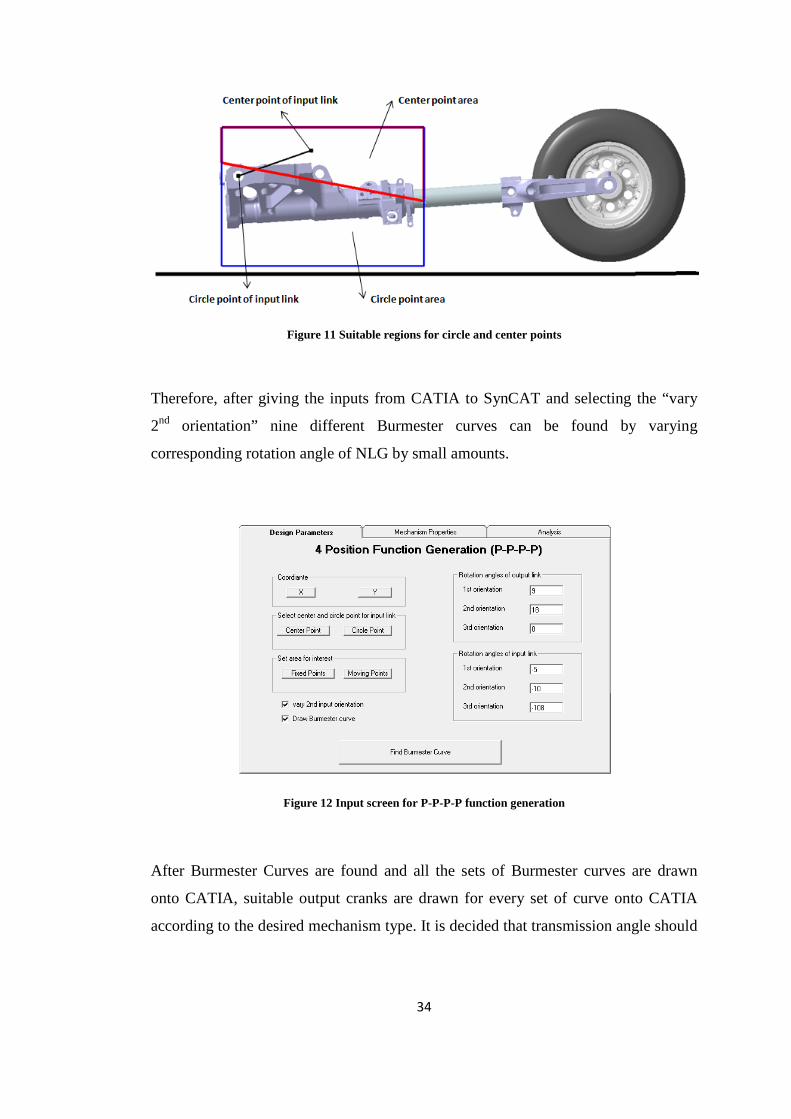
34
Figure 11 Suitable regions for circle and center points
Therefore, after giving the inputs from CATIA to SynCAT and selecting the “vary
2nd orientation” nine different Burmester curves can be found by varying
corresponding rotation angle of NLG by small amounts.
Figure 12 Input screen for P-P-P-P function generation
After Burmester Curves are found and all the sets of Burmester curves are drawn
onto CATIA, suitable output cranks are drawn for every set of curve onto CATIA
according to the desired mechanism type. It is decided that transmission angle should
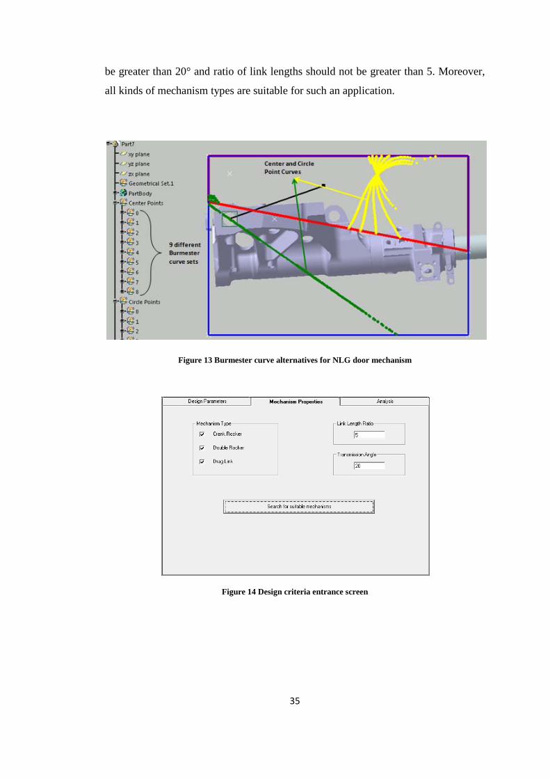
35
be greater than 20° and ratio of link lengths should not be greater than 5. Moreover,
all kinds of mechanism types are suitable for such an application.
Figure 13 Burmester curve alternatives for NLG door mechanism
Figure 14 Design criteria entrance screen
36
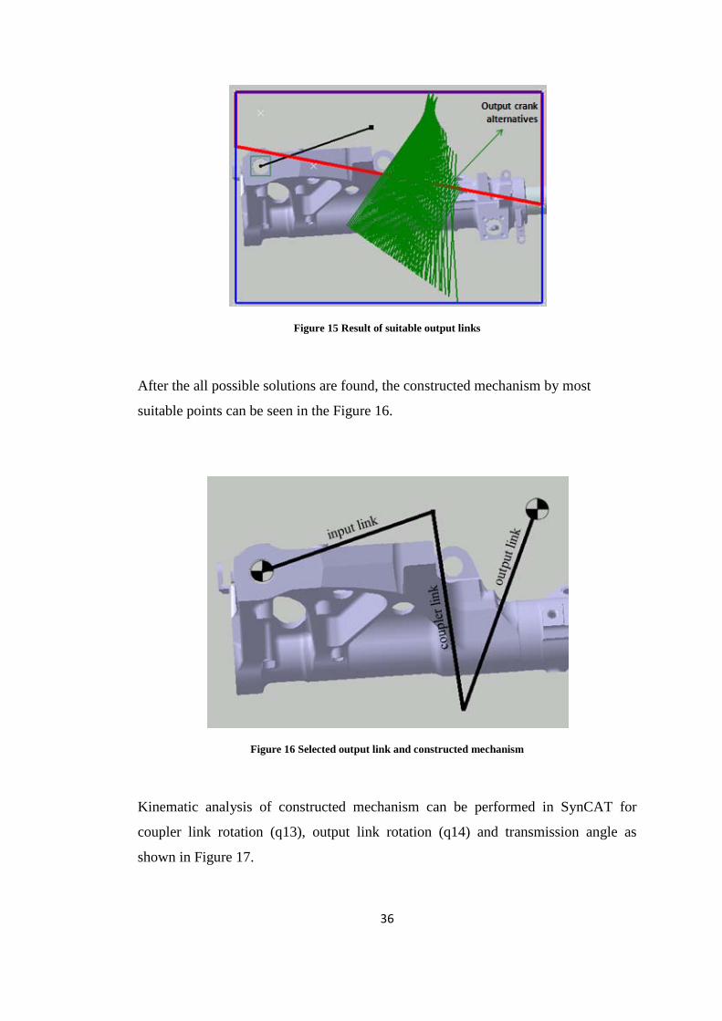
Figure 15 Result of suitable output links
After the all possible solutions are found, the constructed mechanism by most
suitable points can be seen in the Figure 16.
Figure 16 Selected output link and constructed mechanism
Kinematic analysis of constructed mechanism can be performed in SynCAT for
coupler link rotation (q13), output link rotation (q14) and transmission angle as
shown in Figure 17.

37
Figure 17 Kinematic analysis of selected mechanism
Demonstration of whole mechanism can be seen in below table.
Table 10 Motion demonstration of obtained mechanism
NLG Rotation Output
Angle Door
Rotation
0
0 0
-5
9 37
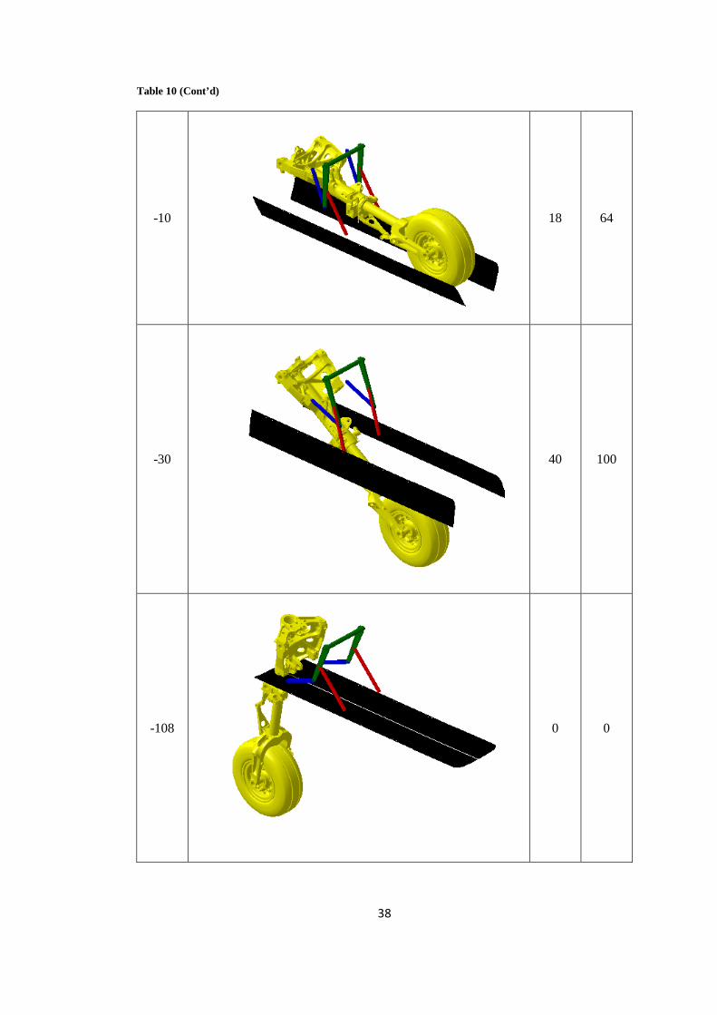
38
Table 10 (Cont’d)
-10
18 64
-30
40 100
-108
0 0
39
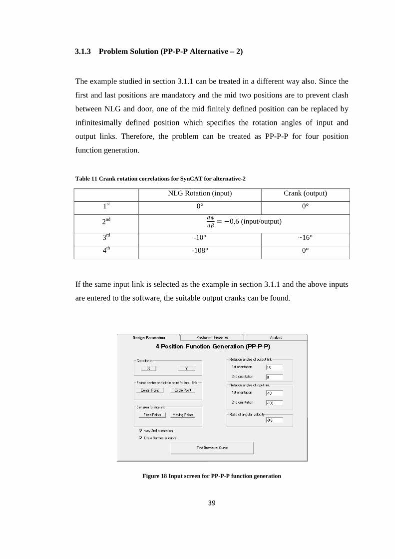
3.1.3 Problem Solution (PP-P-P Alternative – 2)
The example studied in section 3.1.1 can be treated in a different way also. Since the
first and last positions are mandatory and the mid two positions are to prevent clash
between NLG and door, one of the mid finitely defined position can be replaced by
infinitesimally defined position which specifies the rotation angles of input and
output links. Therefore, the problem can be treated as PP-P-P for four position
function generation.
Table 11 Crank rotation correlations for SynCAT for alternative-2
NLG Rotation (input) Crank (output)
1st 0° 0°
2nd 𝑑𝜓𝑑𝛽
= −0,6 (input/output)
3rd -10° ~16°
4th -108° 0°
If the same input link is selected as the example in section 3.1.1 and the above inputs
are entered to the software, the suitable output cranks can be found.
Figure 18 Input screen for PP-P-P function generation

40
Figure 19 Result of suitable output links
If one of the possible output links is selected, mechanism which satisfies desired
conditions can be constructed. Therefore, kinematic analysis of constructed
mechanism can be performed in SynCAT for angular velocity ratio of output link to
input link (w14), coupler link to input link (w13) and rotational angles of output link
(q14), coupler link (q13) as shown in figures below.
Figure 20 Angular position relation of selected mechanism
41
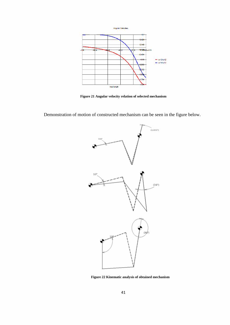
Figure 21 Angular velocity relation of selected mechanism
Demonstration of motion of constructed mechanism can be seen in the figure below.
Figure 22 Kinematic analysis of obtained mechanism

42
3.1.4 Problem Solution (PPP-P Alternative – 3)
The same example can be treated as PPP-P in a third way. The mandatory position is
entered as finitely separated position and the rate of first order of rotation angles of
input and output cranks is given as in order not to have a clash. Finally, the rate of
second order of rotation angles of input and output cranks is given as zero in order to
increase the effect of first order. Therefore following table is used for solution of the
problem;
Table 12 Crank rotation correlations for SynCAT for alternative-3
NLG Rotation (input) Crank (output)
1st 0° 0°
2nd 𝑑𝜓𝑑𝛽
= −0.6 (input/output)
3rd 𝑑2𝜓𝑑𝛽2
= 0 (input/output)
4th -108° 0°
Figure 23 Input screen for PPP-P function generation
If the similar procedure applied at above examples, the possible links can be seen in
below;
43
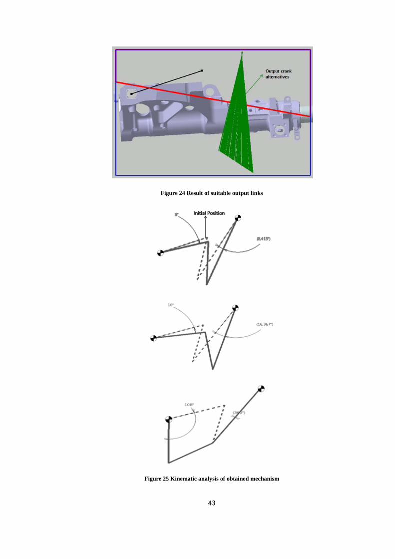
Figure 24 Result of suitable output links
Figure 25 Kinematic analysis of obtained mechanism

44
If one of the possible output links is selected, the angular velocity, rotational
relations between input and output cranks and demonstration of motion can be seen
in the Figure 25. As it can be seen, the ratio between output and finitely prescribed
positions are satisfied.
3.2 FLAP CONTROL SURFACE MECHANISM
3.2.1 Problem Definition
Flap Control Surfaces are the high-lift devices of an aircraft. The aircraft requires
extra lift force at low speeds like take-off or landing conditions and for these
situations different flap positions are required.
The flap positions are determined according to the type and mission of an aircraft
and for this example, the flaps of HURKUS are concerned. The required positions of
flaps are determined as follows;
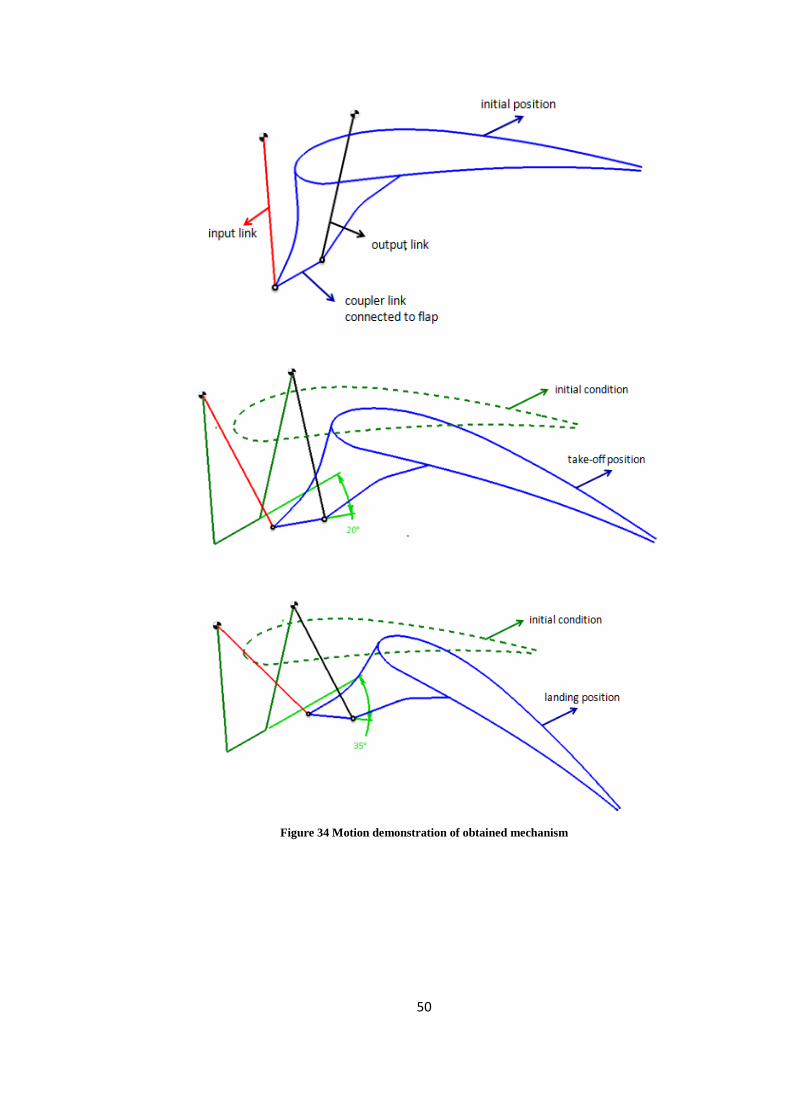
Table 13 Desired flap rotations
Name of Position Flap angle
UP 0°
Take-off (TO) -20°
Landing (LD) -35°
Since the positions are not about an axis, the problem cannot be thought as a function
generation. The problem can be thought as a P-P-P motion generation synthesis,
however, in order to draw a Burmester curve and see the possibilities easier, P-P-P-P
motion generation synthesis will be used for this example by adding an extra flexible
prescribed point. Therefore, the prescribed positions of flap control surface that will
be used in the software are as follows.
45
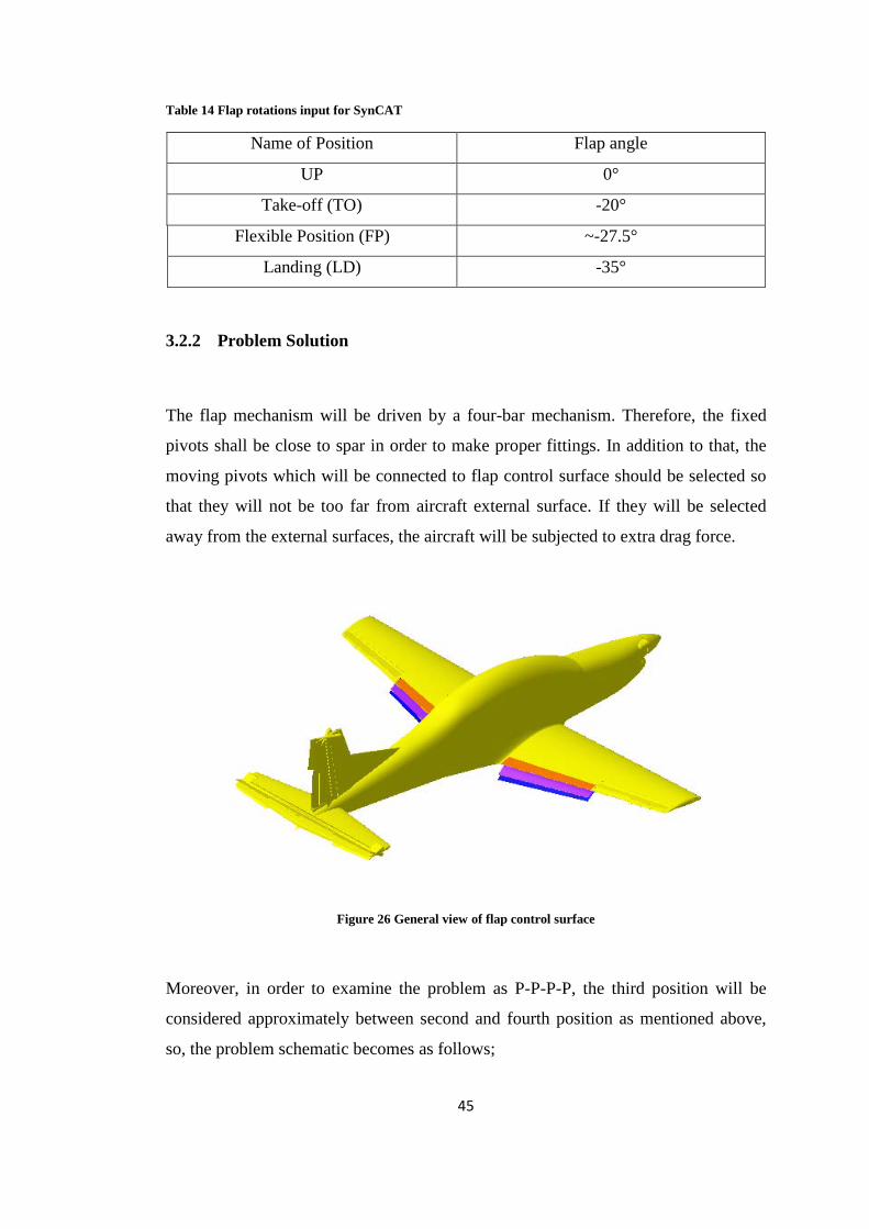
Table 14 Flap rotations input for SynCAT
Name of Position Flap angle
UP 0°
Take-off (TO) -20°
Flexible Position (FP) ~-27.5°
Landing (LD) -35°
3.2.2 Problem Solution
The flap mechanism will be driven by a four-bar mechanism. Therefore, the fixed
pivots shall be close to spar in order to make proper fittings. In addition to that, the
moving pivots which will be connected to flap control surface should be selected so
that they will not be too far from aircraft external surface. If they will be selected
away from the external surfaces, the aircraft will be subjected to extra drag force.
Figure 26 General view of flap control surface
Moreover, in order to examine the problem as P-P-P-P, the third position will be
considered approximately between second and fourth position as mentioned above,
so, the problem schematic becomes as follows;

46
Figure 27 Problem schematic
The red points show the leading edge of the flap at corresponding positions. Then,
designer selects the points from CATIA in the SynCAT and enters the corresponding
flap angles. Moreover, in order to increase the possible mechanism, one can select
“vary 2nd orientation”. By clicking this option, the software will be able to find
different Burmester curve by changing the orientation of flap control surface at the
third position.
Figure 28 Input screen for P-P-P-P motion generation

47
After the positions are determined, the areas for fixed and moving pivots have to be
determined in order to eliminate unwanted mechanism options.
Figure 29 Cross-sectional view of flap control surface and interested regions
Figure 30 Suitable points for moving and fixed points
The area enclosed by green lines is for center points in order to connect them
properly to structure and the area enclosed by the black lines is for circle points. The
area for circle points is not selected bigger in order not to increase drag as mentioned

48
above. Therefore, the eight different Burmester curve is obtained according to the
given inputs as shown in the figure above.
After the Burmester curves are drawn onto CATIA, the designer decide which curve
is most suitable for him and then select the center point for one branch and seek the
other suitable branch by entering the design parameters.
The type of mechanism can be crank-rocker, double rocker or drag-link. In addition
to that, the transmission angle shall not be less than 30 degrees and the link length
ratios shall not be larger than five. According to those design parameters, the
designer can select a circle point from 4th set and find the possible mechanisms.
Figure 31 Design criteria entrance screen
As a result, all possible alternatives are shown in CATIA screen as shown in figure
below. Therefore, the user can build a mechanism by selecting one of possible
output-link which will have a transmission angle greater than 30 degrees during
motion.
49
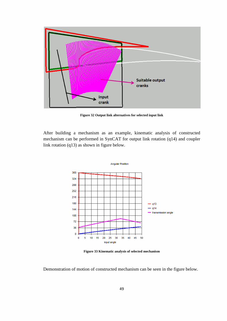
Figure 32 Output link alternatives for selected input link
After building a mechanism as an example, kinematic analysis of constructed mechanism can be performed in SynCAT for output link rotation (q14) and coupler link rotation (q13) as shown in figure below.
Figure 33 Kinematic analysis of selected mechanism
Demonstration of motion of constructed mechanism can be seen in the figure below.
50
Figure 34 Motion demonstration of obtained mechanism
51
3.3 PRIMARY CONTROL SURFACE MECHANISMS
3.3.1 Problem Definition
Primary control surfaces are aileron, elevator and rudder which are mainly used to
give a roll, pitch and yaw motion to an aircraft respectively. These control surfaces
are controlled by the pilot in the cockpit and the motion is generally given by control
stick or pedals. According to the aircraft performance and pilot comfort, the motion
of control surfaces and motion of pedal or stick are determined.
In general, stick or pedal motion is considered as input and the control surface
motion considered as output. Therefore, these mechanisms can be thought as
function generation. As a result, the construction of them can be done by using the
software. However, since the places of control surfaces are far away from the
cockpit, the stick or pedal are connected to control surfaces by many linkages or
cables for some aircrafts which are not fly-by-wire. This software also can be used
for such designs for some portion or for whole of that. In this example, the usage of
this software in such designs will be demonstrated for elevator mechanisms. The
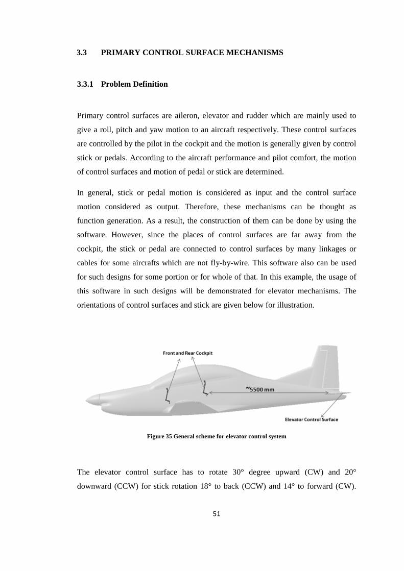
orientations of control surfaces and stick are given below for illustration.
Figure 35 General scheme for elevator control system
The elevator control surface has to rotate 30° degree upward (CW) and 20°
downward (CCW) for stick rotation 18° to back (CCW) and 14° to forward (CW).
52
As seen in the figure, the stick and the elevator are distanced from each other and
they have to be connected with several rods and cables. With the help of push-pull
rods and suitable bell cranks, the desired function correlation will be obtained.
In this design, two four bar mechanism will be constructed and then they will be
connected by cables. The first one will be correlated with the stick motion and the
other one will be correlated with elevator control surface such that the output links of
both mechanisms will rotate same amount, but in different directions in order to
obtain 30° CW rotation of elevator at 18° CCW rotation of stick. In addition to that,
the amount of rotations of cranks will be increased gradually to obtain elevator
control surface rotation. Therefore, the following tables show the orientation of
cranks.
Table 15 First mechanism design input
Stick Rotation 1st Mechanism output link
Lowermost position 14 -20
Neutral 0 0
Approximate position -11 +15
Uppermost position -18 +24
Table 16 Second mechanism design input
Elevator Rotation 2nd Mechanism output link
Lowermost position -20 -20
Neutral 0 0
Approximate position +17 +15
Uppermost position +30 +24
As a result, the mechanisms will be considered at their lowermost position for full
motion. So, the following tables will be used for synthesis problem.
53
Table 17 Summary of the desired motion of mechanism
Stick Rotation 1st Mechanism
output link
Elevator
Rotation
2nd Mechanism
output link
1st orientation -14 20 20 20
2nd orientation -25 35 37 35
3rd orientation -32 44 50 44
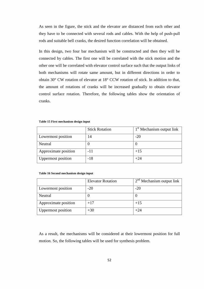
3.3.2 Problem Solution
In the first mechanism, the input link is stick and the suitable area for circle points is
determined according to the allowable space in the fuselage and center points area is
drawn near to floor in order to make proper fitting.
Figure 36 Suitable regions for circle and center points

54
After the rotations of cranks shown in Table 17 and the available areas for circle and
center points entered in the software, designer selects mechanism type and
transmission angle and link length ratio in order to eliminate unwanted results.
Figure 37 Input screen for P-P-P-P function generation
Figure 38 Design criteria entrance screen
After the software is run, the results can be seen in the CATIA screen and with the
most appropriate crank the first four-bar mechanism can be constructed.
55
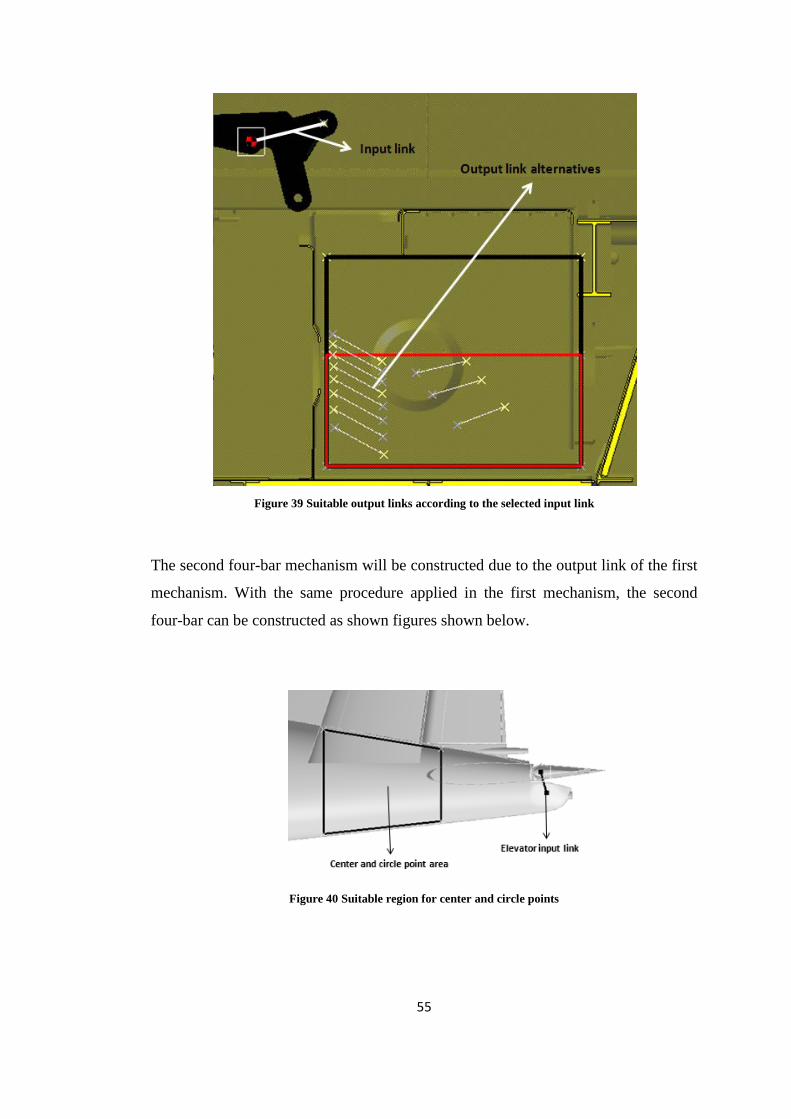
Figure 39 Suitable output links according to the selected input link
The second four-bar mechanism will be constructed due to the output link of the first
mechanism. With the same procedure applied in the first mechanism, the second
four-bar can be constructed as shown figures shown below.
Figure 40 Suitable region for center and circle points

56
Figure 41 Input screen for P-P-P-P function generation
Figure 42 Design criteria entrance screen
Figure 43 Suitable cranks for obtained link

57
As in the first mechanism, with the most appropriate crank, the second four-bar can
be constructed. After that, the first and second mechanism can be connected to each
other by cables, so, that, the synthesis of whole system accomplished.
Figure 44 Demonstration of motion of mechanism
3.4 ACCESS DOOR MECHANISM
3.4.1 Problem Definition
In the air vehicles, there are some removable panels on the outer skin for
maintainability and inspection requirements of parts and equipments. With these
panels, the parts in the air vehicle can be visually checked and/or replaced easily.
These panels can be completely removal or simply hinged to structure or designed
with some properties for some special purposes. These special designed access
panels are generally used for maintainability of large and important equipments like
motor of an aircraft and flir of a helicopter.
In this example, a special access panel for a helicopter will be studied. In this design
the access panel is desired to be opened 90° degree and has to maintain its open
position for disturbances on the access panel for maintainability process. This can be

58
achieved by a four-bar mechanism with its one of the dead center positions. In such a
case, since the system is in a dead-center position, mechanism is not movable by the
inputs given from access panel. The access panel can only be closed by the BB0 link.
Figure 45 Dead-center configuration for four-bar
This position occurs where the angular velocity of the output link changes sign
namely where the angular velocity of a crank is zero. For this problem, there are two
finitely prescribed positions for opened and closed cases. In addition to that, there is
one infinitesimally prescribed position which shows the sign change for opened case.
If one arbitrary finitely prescribed position is selected as an extra, the problem can be
solved for PP-P-P function generation.
3.4.2 Problem Solution
In this problem, since the rotation of access door is defined, one needs to specify a
center point for access door. After that, suitable regions for center and circle points
for other cranks have to be determined.

59
Figure 46 Open configuration for access panel
Figure 47 Closed configuration for access panel
Center point region is selected so that, they will be near to outer skin of helicopter in
order to make a proper fitting (shown in blue in below picture) and they will be
inside the helicopter when the access door is closed. Circle point region is also
selected as they will remain inside the helicopter.
After determining the suitable regions for circle and center points, the prescribed
positions are entered into the software. After a few trials, the arbitrary prescribed
position is determined for most suitable outputs. The following tables summarize the
prescribed positions of the desired mechanism.

60
Figure 48 Suitable regions for center and circle points
Table 18 Input for SynCAT
Access Panel Crank
First Prescribed Position (Opened Case) 0° 0°
Second Prescribed Position �𝑑𝜑𝑑𝛽 �𝛽=0
= 0 (input/output)
Third Prescribed Position (Arbitrary) 45° 70°
Fourth Prescribed Position (Closed Case) 90° 110°
Figure 49 Input screen for PP-P-P function generation

61
As a result, by clicking “draw Burmester curve” options the center and circle points
can be obtained. Designer can select most suitable points and build a four-bar
mechanism which accomplishes the desired task.
Figure 50 Suitable cranks for selected link
After the center and circle points are selected the mechanism can be constructed
which achieves all desired prescribed position as seen in the below figure.
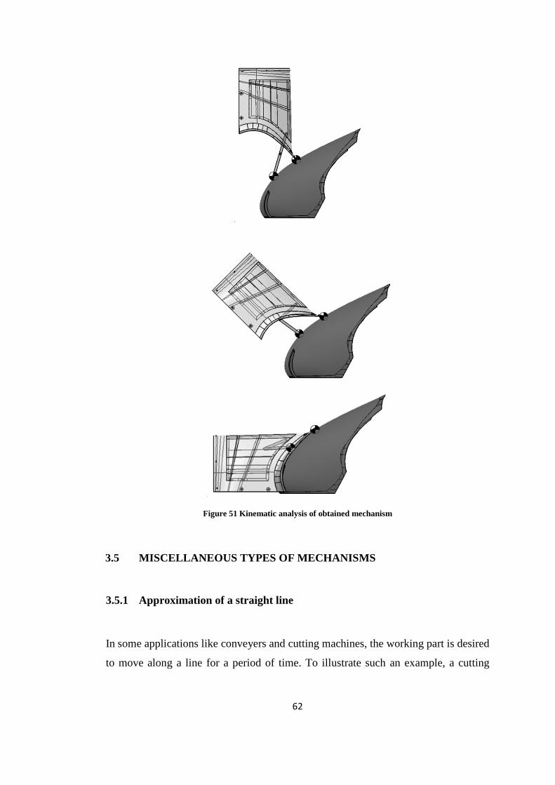
62
Figure 51 Kinematic analysis of obtained mechanism
3.5 MISCELLANEOUS TYPES OF MECHANISMS
3.5.1 Approximation of a straight line
In some applications like conveyers and cutting machines, the working part is desired
to move along a line for a period of time. To illustrate such an example, a cutting
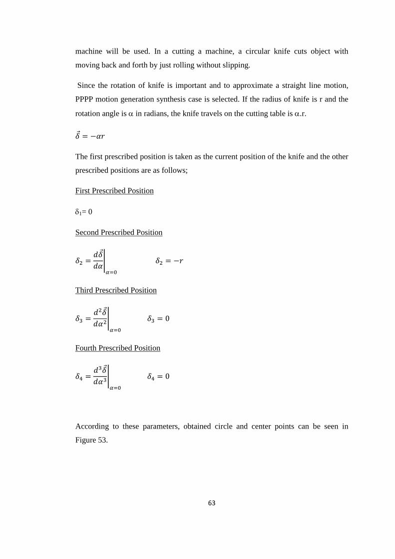
63
machine will be used. In a cutting a machine, a circular knife cuts object with
moving back and forth by just rolling without slipping.
Since the rotation of knife is important and to approximate a straight line motion,
PPPP motion generation synthesis case is selected. If the radius of knife is r and the
rotation angle is α in radians, the knife travels on the cutting table is α.r.
𝛿 = −𝛼𝑟
The first prescribed position is taken as the current position of the knife and the other
prescribed positions are as follows;
First Prescribed Position
δ1= 0
Second Prescribed Position
𝛿2 = �𝑑𝛿𝑑𝛼�𝛼=0
𝛿2 = −𝑟
Third Prescribed Position
𝛿3 = �𝑑2𝛿
𝑑𝛼2�𝛼=0
𝛿3 = 0
Fourth Prescribed Position
𝛿4 = �𝑑3𝛿
𝑑𝛼3�𝛼=0
𝛿4 = 0
According to these parameters, obtained circle and center points can be seen in
Figure 53.

64
Figure 52 Input screen for PPPP motion generation
Figure 53 Center and Circle points for desired mechanism
Therefore, according to the mechanism properties and selected center point for one
branch, the other cranks are obtained. The obtained mechanism can be seen in the
figure below.
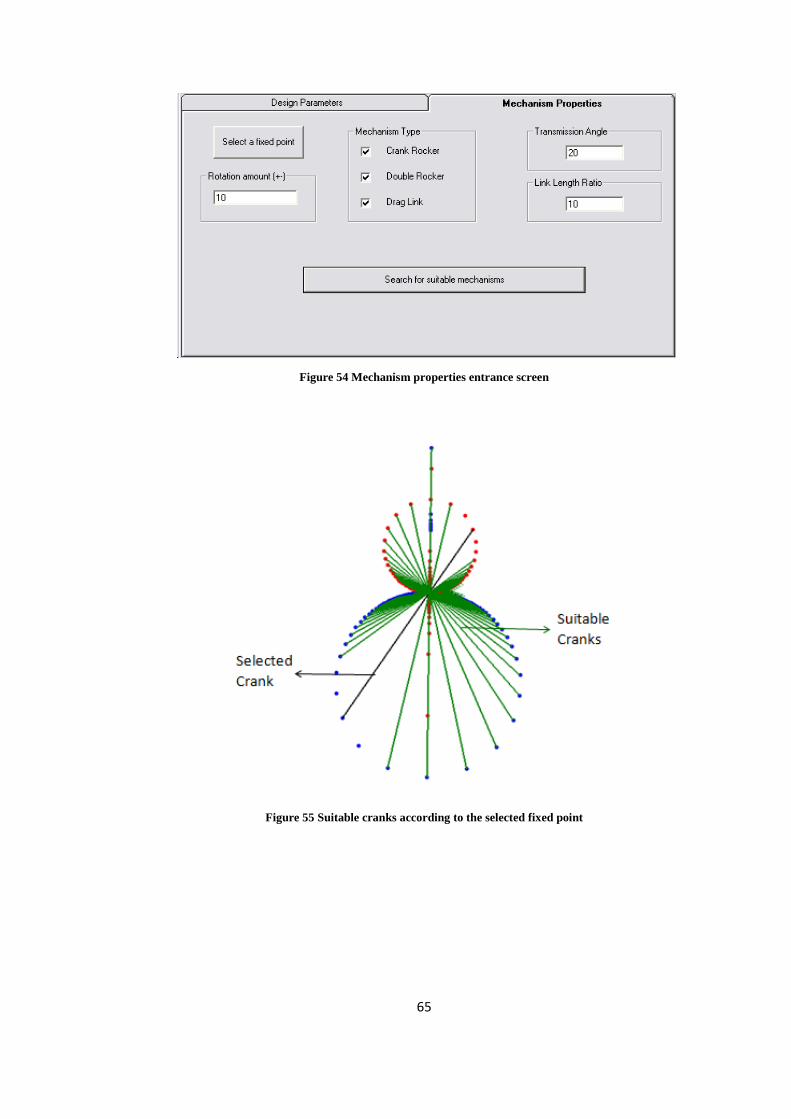
65
Figure 54 Mechanism properties entrance screen
Figure 55 Suitable cranks according to the selected fixed point
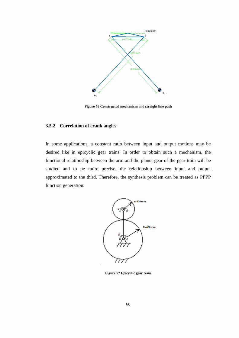
66
Figure 56 Constructed mechanism and straight line path
3.5.2 Correlation of crank angles
In some applications, a constant ratio between input and output motions may be
desired like in epicyclic gear trains. In order to obtain such a mechanism, the
functional relationship between the arm and the planet gear of the gear train will be
studied and to be more precise, the relationship between input and output
approximated to the third. Therefore, the synthesis problem can be treated as PPPP
function generation.
Figure 57 Epicyclic gear train

67
As it can be seen from above figure, with pure rolling condition, the linear relation
relationship between links can be taken as 𝜓 = 𝑅+𝑟𝑟𝛽.
Therefore the prescribed positions are as follows;
First Prescribed Position
δ1= 0
Second Prescribed Position
𝛿2 =𝑑𝜓𝑑𝛽
𝛿2 =𝑅 + 𝑟𝑟
𝛿2 = 3
Third Prescribed Position
𝛿3 =𝑑2𝜓�⃗𝑑𝛽2
𝛿3 = 0
Fourth Prescribed Position
𝛿4 =𝑑3𝜓𝑑𝛽3
𝛿4 = 0
Figure 58 Input entrance screen for PPPP function generation
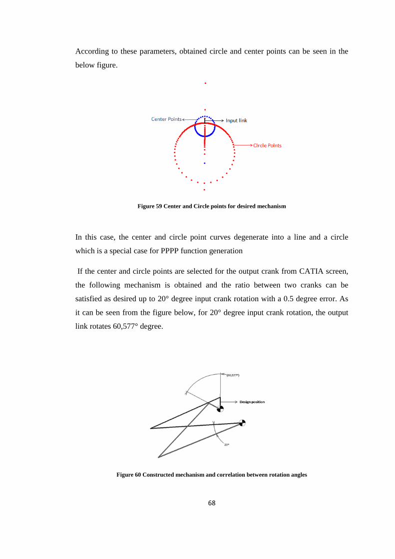
68
According to these parameters, obtained circle and center points can be seen in the
below figure.
Figure 59 Center and Circle points for desired mechanism
In this case, the center and circle point curves degenerate into a line and a circle
which is a special case for PPPP function generation
If the center and circle points are selected for the output crank from CATIA screen,
the following mechanism is obtained and the ratio between two cranks can be
satisfied as desired up to 20° degree input crank rotation with a 0.5 degree error. As
it can be seen from the figure below, for 20° degree input crank rotation, the output
link rotates 60,577° degree.
Figure 60 Constructed mechanism and correlation between rotation angles

69
CHAPTER 4
4. DISCUSSION AND CONCLUSION
4.1 SUMMARY AND DISCUSSION
In this study, visual and interactive computer software package which works with
CATIA V5 in fully parametric form is created for solving aerospace mechanism
synthesis problems. The created software is named as SynCAT and SynCAT is
capable of synthesizing planar four-bar mechanisms for four multiply separated
positions for motion, path and function generation synthesis types.
SynCAT is written in Visual Basic (VB) with graphical user interface since
commands of CATIA V5 is available in VB. Thanks to compatibility with CATIA
and VB, SynCAT performs synthesis of mechanism in CATIA in fully parametric
form. Therefore, designer can use geometrical element in CATIA and get output in
the same design environment.
SynCAT can solve path generation with prescribed timing, function generation and
motion generation problems. Depending on the problem to be solved, different inputs
must be provided to the program. Therefore, after design parameters are given as the
input, SynCAT is capable of drawing Burmester curve exactly for design parameters
or Burmester curves by varying one of the design parameter.
Furthermore, SynCAT has been tested for several aerospace applications and six of
them explained in this thesis in details. During testing these examples in SynCAT, no
problems are encountered and synthesis of these mechanisms is performed.

70
4.2 FUTURE WORKS
In dyadic approach, Burmester curves are found by varying one of the independent
parameters with a certain increment. For example, in motion generation problem,
there are three different independent variables namely the crank angle in one of the
design positions: β2, β3, β4 and SynCAT determines the resulting Burmester curves
by varying β2 from 0 to 360 with a fixed increment. The resulting points found on the
circle and center point curves may be too close or too far apart. This problem can be
eliminated by changing the increment and/or the independent parameter. In such a
method the software may check the distances between two consecutive points and
increase or decrease the increment if the distances are not in the specified range or
change the independent parameter to another crank angle such as β3. Therefore, with
this improvement, points that can’t be found with fixed increment can be determined.
.
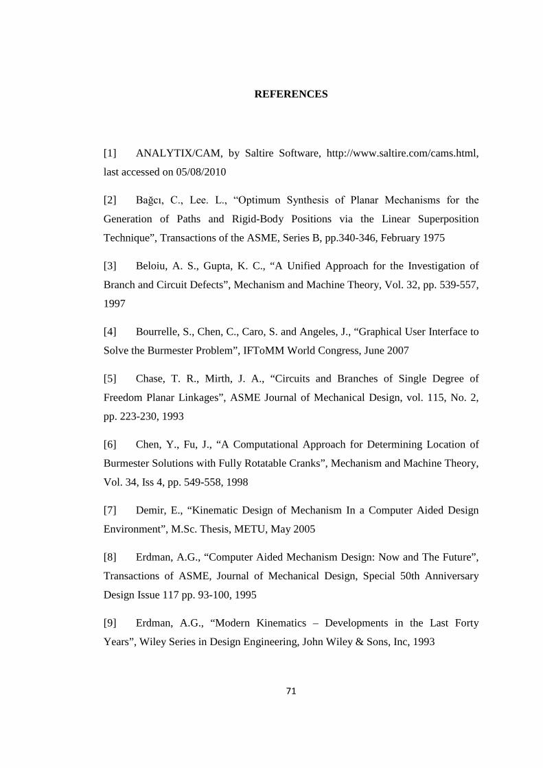
71
REFERENCES
[1] ANALYTIX/CAM, by Saltire Software, http://www.saltire.com/cams.html,
last accessed on 05/08/2010
[2] Bağcı, C., Lee. L., “Optimum Synthesis of Planar Mechanisms for the
Generation of Paths and Rigid-Body Positions via the Linear Superposition
Technique”, Transactions of the ASME, Series B, pp.340-346, February 1975
[3] Beloiu, A. S., Gupta, K. C., “A Unified Approach for the Investigation of
Branch and Circuit Defects”, Mechanism and Machine Theory, Vol. 32, pp. 539-557,
1997
[4] Bourrelle, S., Chen, C., Caro, S. and Angeles, J., “Graphical User Interface to
Solve the Burmester Problem”, IFToMM World Congress, June 2007
[5] Chase, T. R., Mirth, J. A., “Circuits and Branches of Single Degree of
Freedom Planar Linkages”, ASME Journal of Mechanical Design, vol. 115, No. 2,
pp. 223-230, 1993
[6] Chen, Y., Fu, J., “A Computational Approach for Determining Location of
Burmester Solutions with Fully Rotatable Cranks”, Mechanism and Machine Theory,
Vol. 34, Iss 4, pp. 549-558, 1998
[7] Demir, E., “Kinematic Design of Mechanism In a Computer Aided Design
Environment”, M.Sc. Thesis, METU, May 2005
[8] Erdman, A.G., “Computer Aided Mechanism Design: Now and The Future”,
Transactions of ASME, Journal of Mechanical Design, Special 50th Anniversary
Design Issue 117 pp. 93-100, 1995
[9] Erdman, A.G., “Modern Kinematics – Developments in the Last Forty
Years”, Wiley Series in Design Engineering, John Wiley & Sons, Inc, 1993
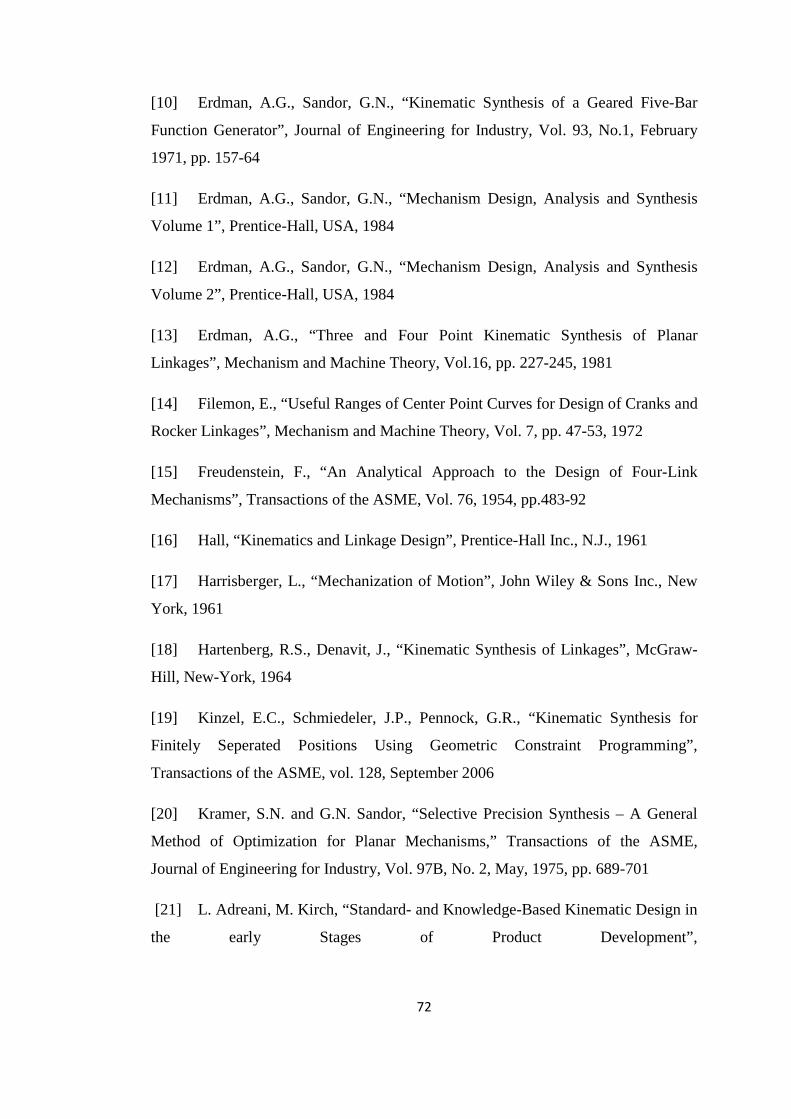
72
[10] Erdman, A.G., Sandor, G.N., “Kinematic Synthesis of a Geared Five-Bar
Function Generator”, Journal of Engineering for Industry, Vol. 93, No.1, February
1971, pp. 157-64
[11] Erdman, A.G., Sandor, G.N., “Mechanism Design, Analysis and Synthesis
Volume 1”, Prentice-Hall, USA, 1984
[12] Erdman, A.G., Sandor, G.N., “Mechanism Design, Analysis and Synthesis
Volume 2”, Prentice-Hall, USA, 1984
[13] Erdman, A.G., “Three and Four Point Kinematic Synthesis of Planar
Linkages”, Mechanism and Machine Theory, Vol.16, pp. 227-245, 1981
[14] Filemon, E., “Useful Ranges of Center Point Curves for Design of Cranks and
Rocker Linkages”, Mechanism and Machine Theory, Vol. 7, pp. 47-53, 1972
[15] Freudenstein, F., “An Analytical Approach to the Design of Four-Link
Mechanisms”, Transactions of the ASME, Vol. 76, 1954, pp.483-92
[16] Hall, “Kinematics and Linkage Design”, Prentice-Hall Inc., N.J., 1961
[17] Harrisberger, L., “Mechanization of Motion”, John Wiley & Sons Inc., New
York, 1961
[18] Hartenberg, R.S., Denavit, J., “Kinematic Synthesis of Linkages”, McGraw-
Hill, New-York, 1964
[19] Kinzel, E.C., Schmiedeler, J.P., Pennock, G.R., “Kinematic Synthesis for
Finitely Seperated Positions Using Geometric Constraint Programming”,
Transactions of the ASME, vol. 128, September 2006
[20] Kramer, S.N. and G.N. Sandor, “Selective Precision Synthesis – A General
Method of Optimization for Planar Mechanisms,” Transactions of the ASME,
Journal of Engineering for Industry, Vol. 97B, No. 2, May, 1975, pp. 689-701
[21] L. Adreani, M. Kirch, “Standard- and Knowledge-Based Kinematic Design in
the early Stages of Product Development”,

73
http://www.prostep.org/en/events/symposium-2008/program/09042008, last accessed
on 11/09/2010
[22] LINCAGES: Linkage INteractive Computer Assisted Geometrically
Enhanced Synthesis, http://www.me.umn.edu/labs/lincages/, last accessed on
28/04/2011
[23] Martin P.J., Russell K., Sodhi R.S., “On mechanism design optimization for
motion generation”, Mechanism and Machine Theory, November, 2006
[24] N.B., Talekar, T. DePauw, “Kinematic Synthesis (Function Generation) in
Adams/View”, International Adams Conferance, 1998
[25] P. Larochelle, J. Dooley, A. Murray, J.M. McCarthy, “SPHINX-Software for
Synthesizing Spherical 4R Mechanisms”, University of California
[26] Polat, M., “Computer Aided Synthesis of Planar Mechanisms”, M.Sc. Thesis,
METU, March 1985
[27] Reuleaux, F., “The Kinematic of Machinery-Outline of a Theory of
Machines”, Translated by A.B. W. Kennedy, MacMillan and Co., London, 1876
[28] Sandor, G.N., “A General Complex Number Method for Plane Kinematic
Synthesis with Applications”, Doctoral Dissertation, Columbia University
Microfilms, Ann Arbor, 305 pp., LCC No. Mic 59-2596, 1959
[29] Schaefer, R.S., Kramer, S.N., “Selective Precision Synthesis of Planar
Mechanisms Satisfying Position and Velocity Constraints”, Mechanism and Machine
Theory, Vol.14, pp. 161-170, 1979
[30] Sezen, S.A., “Development of An Interactive Visual Planar Mechanism
Synthesis and Analysis Program By Using Delphi Object Oriented Programming
Environment”, M.Sc. Thesis, METU, June, 2001
[31] Synthetica, http://www.umbc.edu/engineering/me/vrml/research/software/,
last accessed on 01/03/2011
74
[32] Tesar, D., Eschenbach, W., “Four Multiply Separated Positions in Coplanar
Motion”, Journal of Engineering for Industry, pp. 231-234, May 1967
[33] Tesar, D., “The Generalized Concept of Three Multiply Separated Positions
in Coplanar Motion”, Journal of Mechanisms, Vol.2, pp. 462-474, 1967
[34] Waldron, K.J., “Graphical Solution of The Branch and Order Problems of
Linkage Synthesis for Multiply Separated Positions”, Journal of Engineering for
Industry, 1977, pp. 591-597
[35] Waldron, K.J., “Location of Burmester Synthesis with Fully Rotatable
Cranks”, Mechanism and Machine Theory, 1978, Vol.13, pp. 125-137
[36] Waldron, K.J., “Range of Joint Rotations in Planar Four-Bar Synthesis for
Finitely Seperated Position Part-I The Multiple Branch Problem” ASME Paper No.
74-DET-108, Mechanisms Conference, New York, 1974
[37] WATT, Mechanism Design Suite, by Heron Technologies,
http://www.heron.com, last accessed on 20/05/2010
[38] Y. Chen, J. Fu, “A computational approach for determining location of
Burmester solutions with fully rotatable cranks”, Mechanism and Machine Theory,
1999, pp. 549-558

75
APPENDIX A
FLOWCHART OF SynCAT
Figure 61 Flowchart of SynCAT

76
APPENDIX B
OBTAINING COORDINATES OF A POINT FROM CATIA
Sub CATgetcoord(point_name$, p1$, p2$, p3$)
Set CATIA = GetObject(, "CATIA.Application")
Set PartDocument = CATIA.ActiveDocument
Set Selection = PartDocument.Selection
Dim Point As Variant
MsgBox "Select a Point for" & point_name$
Set Point = Selection.Item(1).Value
ReDim koord(2)
Point.GetCoordinates koord
p1 = koord(0) ‘X coord
p2 = koord(1) ‘Y coord
p3 = koord(2) ‘Z coord
End Sub

77
APPENDIX C
PRINTING POINT ONTO CATIA
Set CATIA = GetObject(, "CATIA.Application")
Set partDocument1 = CATIA.ActiveDocument
Set Part1 = partDocument1.Part
Set hybridBodies1 = Part1.HybridBodies
Set hybridBody1 = hybridBodies1.Add()
hybridBody1.Name = "Center Points" ‘naming of the geometrical set
Set hybridShapeFactory1 = Part1.HybridShapeFactory
Set Point_1 = hybridShapeFactory1.AddNewPointCoord(X,Y,Z)
hybridBody1.AppendHybridShape Point_1
Part1.InWorkObject = Point_1

78
APPENDIX D
PRINTING LINE ONTO CATIA
Set CATIA = GetObject(, "CATIA.Application")
Set partDocument1 = CATIA.ActiveDocument
Set Part1 = partDocument1.Part
Set hybridBodies1 = Part1.HybridBodies
Set hybridBody1 = hybridBodies1.Add()
hybridBody1.Name = "Crank-Rocker alternatives" ‘naming geometrical set
Set hybridShapeFactory1 = Part1.HybridShapeFactory
Set Point_B0 = hybridShapeFactory1.AddNewPointCoord(X1,Y1,Z1)
Set Point_B = hybridShapeFactory1.AddNewPointCoord(X2,Y2,Z2)
Set reference1 = Part1.CreateReferenceFromObject(Point_B0)
Set reference2 = Part1.CreateReferenceFromObject(Point_B)
Set Line_1 = hybridShapeFactory1.AddNewLinePtPt(reference1, reference2)
hybridBody1.AppendHybridShape Line_1
Line_1.Name = "output crank"
Part1.InWorkObject = Line_1
Part1.Update


