
Harvard Institute forInternational Development
HARVARD UNIVERSITY
An Integrated Analysis of a PowerPurchase Agreement
Glenn P. Jenkins and Henry B.F. Lim
Development Discussion Paper No. 691April 1999
© Copyright 1999 Glenn P. Jenkins, Henry B.F. Lim,and President and Fellows of Harvard College
Development Discussion Papers
HIID Development Discussion Paper no. 691
An Integrated Analysis of a Power Purchase Agreement
Glenn P. Jenkins and Henry B.F. Lim
Abstract
A Power Purchase Agreement (PPA) is at the heart of any BOT or BOO type power generationproject that is to be undertaken by an Independent Power Producer (IPP). During the past decadeprivately owned IPPs selling electricity to the power industry has become common place. Sucharrangements require some version of a PPA. In this paper we model a multi-currency loan andequity financing package for a 100 MW combined-cycle gas turbine generation plant that is to bebuilt in India. Using this financial model we evaluate a sophisticated power purchase agreementin order to identify the relative importance of each of the variables found in such an agreement.Variables become important if they represent major elements of costs or revenues or aresignificant sources of risk.
This paper provides an example of the benefits that an integrated financial-economic-stakeholder analysis can bring to the evaluation of a PPA and BOT contracts. The integratedapproach allows various scenarios to be compared from different perspectives and points ofview. The economic analysis looks at the project’s impact on a country’s overall economy. Thefinancial analysis of such an infrastructure project checks on the profitability and sustainabilityof the project over time. Sensitivity and risk analyses are central to the evaluation of this projectsince they identify the most critical variables and allow a probability distribution of values to beused in the model, rather than a single predicted value. The distributive or stakeholder analysisidentifies who would be the major winners and losers if the power plant project were undertaken.This approach enables the partners to the agreement to “test” the sustainability of the contractthrough the analysis of the project’s outcomes under a wide range of situations and combinationsof scenarios before the PPA is entered into. The technique of testing contracts for their futuresustainability is area of research of potentially great benefit to the parties entering into long termcontractual arrangements for public services.
JEL Codes: D61, H43, L94
Keywords: India, electricity, agreement, foreign investment, privatization, appraisal.
Glenn Jenkins is an Institute Fellow and Director of the Program on Investment Appraisal andManagement at HIID, and Director of the International Tax Program at Harvard Law School.
Henry Lim is a Research Fellow at the International Tax Program, Harvard Law School.
HIID Development Discussion Paper no. 691
An Integrated Analysis of a Power Purchase Agreement
Glenn P. Jenkins and Henry B.F. Lim 1
I. INTRODUCTION
The Indian government, in their 1992 five-year development plan stated that the country
would need 142,000 MW of power capacity by the year 2005. This would require an additional
48,000 MW of electrical generating capacity to the existing 75,000 MW. In the 1990’s the rate of
economic growth in India accelerated from near stagnation in 1990-1992 to 6% in 1993-1994,
6.3% in 1994-1995 and 6% in 1995-1996. If the electrical energy demanded is not supplied, this
experience of improved economic performance could be put in jeopardy.
In 1992, the government amended India’s Electricity Act of 1910 and opened the
electricity sector to privatization and foreign investment. An incentive package was enacted in
1993 to provide a five year tax holiday for new projects in the power sector and a guaranteed
16% return on foreign investment. Additionally, the protracted project approval system was
substantially revised. In January 1996, the government announced new guidelines governing
how India’s state-run electricity boards should evaluate their power projects through competitive
bidding. Even though the states have the responsibility for negotiating their own power deals,
they are likely to follow the new guidelines, as the federal power ministry’s approval is required
for all new projects.
The state of Sendara Pradesh2 requires substantial additions to its present power
generating capacity to meet the power demands of its growing industry, agriculture and other
sectors. For the period 1998-2000, the shortfalls in peak capacity are 1,471 MW, 2,035 MW and
2,263 MW. The state is experiencing an acute shortage of power to a point where there has been
1 The collaboration of José F. Azpurua Sosa and Alberto Barreix in the completion of this study was essential,
and greatly appreciated. The comments of our colleagues, Baher El-Hifwani, D.N.S. Dhakal, G.P. Shukla andMigara Jayawardena have helped to enhance the analysis. A special thanks to the participants of the ProgramAppraisal and Risk Analysis for the Power Sector, held at the National Institute for Financial ManagementFaridabad India in January 1998, who provided us with many insights on the role and operation of Power PurchaseAgreements in India. Any errors that remain are the responsibility of the authors alone.

2
frequent power failures as well as demand cuts on high-voltage industrial customers and
restrictions on low-voltage businesses and residential customers during peak hours. This trend
has to be reversed to satisfy the unrestricted demand of power and to provide adequate reserves
for periodic overhauls and emergency outages. The Sendara Pradesh State Electricity Board
(SPSEB) has already identified a number of industrial projects that have been stalled at various
stages of implementation due to power shortages. For a large part of the state, the supply of
adequate electricity is an immediate requirement for industrial development and for improving
the living conditions of the people. By the year 2000, the State of Sendara Pradesh is expected to
face a deficit of 2,263 MW in peak power availability. The Government of Sendara Pradesh is
encouraging several private power developers to participate in the construction of new power
plants within the shortest possible time.
As a result of this policy, a Memorandum of Understanding (MOU) was signed between
the Government of Sendara Pradesh, Sendara Pradesh State Electricity Board (SPSEB),
Industrial Power Supply Private Limited (IPS) and Edison-Madison Electric Company Private
Limited . IPS and Edison-Madison are hereby collectively known as Sendara Pradesh Power
Partners Private Limited (SPPL), which is a joint stock company with equity participation,
registered by IPS and Edison-Madison to develop, finance, build, operate and transfer an
approximately 100 MW power plant on an exclusive basis under the terms of the MOU.
The purpose of this paper is to build an intergrated financial, economic, and stakeholder
model of this project and to use this case to illustrate the use of this set of tools for the
assessment of the specific outcomes and risks for such arrangements.
2 In order to preserve the confidentiality of the project, the names of the state and the various interested parties
have been changed.

3
II. PROJECT DESCRIPTION
A. Project Objectives and Scope
The plant will be located at the site of an old decommissioned 10 MW coal-fired thermal
power station. The new facility is designed to provide approximately 106 MW of capacity at the
generator terminals.
The SPPL Power Project includes the following components:
(1) Construction in about 18 months of a Naphtha-based open/cogeneration/combinedcycle generation plant of 100-140 MW capacity.
(2) Refurbishment and renovation of the railway siding for use of transportation ofresidual fuel oil or naphtha and other distillates. Appropriate logistical arrangements to bemade for ensuring a continuous and reliable supply of fuel to the project.
(3) Ground water is available at a depth of about 150 ft and it can be presumed thatminimum consumption requirement for closed cycle cooling arrangement can be met fromthe deep borewells.
(4) Demolition and clearance of existing plants, buildings, and machinery on the site.
(5) For feeding the power from proposed station to the grid, the existing 132 kVswitchyard has to be extended with additional step-up transformers and outgoing feeders.
(6 ) Measures are to be undertaken to mitigate the project's impact on the environment.
B. Project Cost and Financing
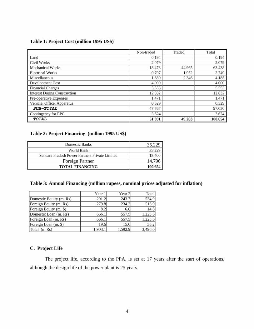
The total cost of the project in 1995 US dollars is estimated at US$100.654 million, with
the traded component of costs equal to US$49.263 million (Table 1). The cost estimates are
based on actual prices obtained through international competitive bidding. The cost estimates
provide for both physical and price contingencies.
Domestic banks and the World Bank will finance the project through two loans of
US$35.23 million each at 6.48% and 5.34% percent real rate of interest, respectively. SPPL’s
private partners will provide the balance of US$31.2 million with equity.
4
Table 1: Project Cost (million 1995 US$)
Non-traded Traded TotalLand 0.194 0.194Civil Works 2.079 2.079Mechanical Works 18.473 44.965 63.438Electrical Works 0.797 1.952 2.749Miscellaneous 1.839 2.346 4.185Development Cost 4.000 4.000Financial Charges 5.553 5.553Interest During Construction 12.832 12.832Pre-operative Expenses 1.471 1.471Vehicle, Office, Apparatus 0.529 0.529SUB-TOTAL 47.767 97.030
Contingency for EPC 3.624 3.624TOTAL 51.391 49.263 100.654
Table 2: Project Financing (million 1995 US$)
Domestic Banks 35.229World Bank 35.229
Sendara Pradesh Power Partners Private Limited 15.400
Foreign Partner 14.796TOTAL FINANCING 100.654
Table 3: Annual Financing (million rupees, nominal prices adjusted for inflation)
Year 1 Year 2 TotalDomestic Equity (m. Rs) 291.2 243.7 534.9Foreign Equity (m. Rs) 279.8 234.2 513.9Foreign Equity (m. $) 8.2 6.6 14.8Domestic Loan (m. Rs) 666.1 557.5 1,223.6Foreign Loan (m. Rs) 666.1 557.5 1,223.6Foreign Loan (m. $) 19.6 15.6 35.2Total (m Rs) 1,903.1 1,592.9 3,496.0
C. Project Life
The project life, according to the PPA, is set at 17 years after the start of operations,
although the design life of the power plant is 25 years.
5
D. Project Implementation and Management
The project will be implemented by SPPL, which will contract management services in
the first years, until local employees are able to manage the project. SPSEB will regulate its
activities and purchase its output.
III. THE POWER PURCHASE AGREEMENT
The PPA signed between SPPL and SPSEB is a fixed rate of return (ROE) type that
specifies how SPPL will be paid for the electricity to be delivered by the SPPL plant for a period
of 17 years after which the plant will be transferred to SPSEB at a negotiated transfer price. This
type of contract is not unique to India, but has become one of the standard format contracts used
internationally. The PPA consists of four major payment categories: (i) fixed charge payment,
(ii) variable charge payment, (iii) incentive payment, and (iv) transfer price.
A. Fixed Charge Payment
For a PPA of the fixed-ROE (fixed Rate Of Return) type, the fixed charge payment is
usually the most important category of the major payment categories. This fixed charge payment
category includes the following payments:
(1) Interest on Debt,(2) Depreciation Payment,(3) Return on Equity,(4) Interest on Working Capital,(5) O&M and Insurance Expenses3,(6) Taxes on Income,(7) Special Appropriation.
Except for the fifth and sixth items, these payments are the major vehicle from which the
IPP will recover its investment costs plus a return on its equity. Based on the actual design of the
PPA, the IPP partners may actually earn more or less than the fixed ROE explicitly specified in
3 Whether O&M plus insurance truly reflects the actual costs could have a significant impact of the project
NPVs.

6
the agreement.4 A power purchase agreement (the PPA) signed between an electric utility or a
state electricity board and an IPP is usually based on a fixed return on equity. Accordingly, the
IPP is guaranteed a fixed return, 16% in India, on the partners’ equity. Whether this 16% ROE
is a real or a nominal rate of return is usually not specified in a PPA. It is nevertheless a
common practice to treat it as a nominal ROE. The real ROE will therefore depend on the rate of
inflation experienced during the duration of the contract5.
The definition of all the items listed above are all reasonably transparent except for thedepreciation payment and special appropriation components. The depreciation payment isdefined as:
(1) . n
RVR)- (1 C DP
or
, Periodsion DepreciatofNumber
Ratio)Value Residual- (1 Cost Investment er Period Payment Pion Depreciat
×=
×=
The residual value ratio (RVR) is the portion of the investment cost that will not be
depreciated. This undepreciated portion is supposed to be recouped by the transfer price at the
consummation of the contract. The annual depreciation payment per period is a function of RVR
and the number years over which the depreciation payments are made (n). If the RVR and n are
low, the depreciation payment is “front-end-loaded”. This can increase the project’s NPV from
the IPP point of view.
Whenever the repayment of the principals of the loans obtained by the project exceeds
the depreciation payment, the utility is required to pay a “special appropriation” whose amount is
4 The ROE specified in the PPA is only part of a payment package as noted in the fixed charge payments. It may
differ significantly from the actual return on equity that the IPP partners would get.5 If a domestic inflation of 8% were expected, as in our base case for India, then the underlying real ROE in
rupees would be 7.41%. But if the rate of inflation were 3% as is assigned for the U.S., the underlying real ROEwould be 12.62% on dollar-dominated equity financing.

7
equal to the difference between the two. Depending on how the loans are structured, this item
can have a significant impact on the project’s, the utility’s and the equity holders’ NPVs.
The combination of the depreciation and the special appropriation payments are subjected
to two further restrictions: (1) the accumulated sum of the depreciation and the special
appropriation payments is not to exceed (1-RVR)*total investment cost, and (2) that after all
debts are repaid, the total fixed charge for each period will be reduced by an amount, which will
be referred to as “Fixed Charge Adjustment I” in our case study, equal to:
×=
debt total- paymentsion appropriat special
ondepreciati theof sum dAccumulate Rate Prime I Adjustment Charge Fixed 6 (2)
In other words, the prime interest rate will be paid to the electricity board on any
payments it has made to the IPP in excess of the amount of debt financing less the residual value.
In the event that the calculated plant load factor (CPLF) is less than the Normative Plant Load
Factor (NPLF), the total fixed charge payment will be reduced by an amount equal to the
following:
NPLF CPLF if , NPLF
CPLF - 1 Payment Charge FixedII Adjustment Carge Fixed <
×= 7 (3)
6 The Depreciation and Special Appropriation payments are restricted by, for example, the following statement
from one of the PPAs. “ `Depreciation’ shall mean the depreciation on the assets of the Project based on the CapitalCost at the rates specified by the Government of India as of the date of this Agreement under the Electricity Laws;provided, however, that the allowance for depreciation shall be zero from and after the date on which the aggregateof all payments for Depreciation and Special Appropriation equals 90% of the Capital Cost, provided further,however, that with respect to each Billing Period after the Billing period in which the Debt is due to be fully repaidin accordance with the Debt Amortization Schedules, the applicable Fixed Charge Payment shall be further reducedby an amount equal to the interest (calculated at the prime lending rate of the State Bank of India) on the amount bywhich the aggregate amount of Depreciation and Special Appropriation provided for pursuant to this Appendix Dexceeds the aggregate amount of Debt referred to in the Financing Plan.” If the Depreciation and SpecialAppropriation payments are not restricted by the preceding conditions, they will result in excessive over-repaymentof the total investment cost.
7 CPLF is defined as (actual energy delivered + deemed generation)/(capacity*hours of period). NormativePLF is supposedly the average PLF for a specific plant operates under normal conditions. In India, however, NPLFis specified by the Indian Government PPA directives. See also Incentive Payment below.

8
B. Variable Charge Payment
The variable charge payment is a payment for the fuel costs actually incurred by the
plant.8
C. Incentive Payment
Inventive payment is defined as:
( ) (4) , .6849 CPLF if , 365
n 100 .6849 - CPLF .007 Equity Payment Inventive >
××××=
where n is the number of days in the Billing Period, 68.49 is the Normative PLF (NPLF)9 and
.007 (.7 of 1%) is the incentive points. Both the NPLF and the incentive points are negotiated
values, with the values shown here being those specific to this contract.
IV. APPRAISAL OF THE SPPL PROJECT FROM DIFFERENT POINTS OF VIEW
It is customary to look at a project from the different perspectives - total investment,
equity owner, and economic. This approach can be applied to any project. The different
stakeholder points of view - the utility versus the IPP, which are explained below, apply only to
specific situations such as the present case of a PPA which is also part of a BOT agreement.
A. The Utility (SPSEB) Point of View
Traditionally, the most important mandate of a utility is to provide reliable power at the
lowest cost. This role has more or less been fulfilled by the traditional utilities when they are
regulated and managed properly. Recent changes have altered some of the attributes of this
traditional mandate. These changes have arisen because of the introduction of privatization and
8 How to provide incentives for the IPP to minimize fuel costs is crucial but often omitted in most PPAs.9 Normative PLF is the PLF expected for the plant under normal conditions. It is to be agreed by the Utility and
the IPP.

9
competition with the intent to widen financing capability and reduce costs. The latter is often
referred to as “deregulation”. Another important change is the rapid growth of many developing
countries, which has led to a shortage of public funds to meet the expanding demand for basic
infrastructure such as transportation, communications, electricity, and others. The combination
of privatization, competition and the shortage of investment funds has led to the introduction of
many BOT projects as a substitute for the traditional publicly funded projects in these sectors.
The biggest attraction of a BOT deal to a utility, through the signing of a PPA, is the
avoidance of having to raise the funds to finance generation capacity. However, from the point
of view of a utility, or any buyer of electricity, reliable power at a reasonable price remains one
of the most important criteria. An investment appraisal is one way to ascertain if the price paid
for the electricity is reasonable. For example, the utility would like to know what is the ROE that
would satisfy the IPP and at the same time not give the IPP a return that is significantly greater
than the minimum required to attract an IPP with the needed skills and resources. It also needs to
know what is the true rate of return to the IPP10, or alternatively what is the impact of the key
negotiation variables on the financial NPV.
For a fixed-ROE PPA, there are many specifications and variables that have to be
negotiated between the two parties. Among the many contract items, the key variables are the
ROE, the capital cost, the normative plant load factor (NPLF), the incentive points, the
depreciation payment scheme, the calculation of O&M plus insurance payment, the special
appropriation, and the variable charge payment.
When the utility is also a parastatal enterprise such as the SPSEB, various parts of the
agreement may be benefited from public guarantees or subsidies. The investment appraisal
should also consider the economic costs and benefits of the project even though the financial
viability and constraints may be the overriding concerns.
10 The true rate of return to the IPP is the real rate of discount at which the real financial NPV is equal to zero.
10
B. The IPP (SPPL) Point Of View
From the IPP’s point of view, the true financial return of the project is its main concern.
Hence an IPP will use the results of the financial analysis to set its minimum-return positions
while striving for the maximum return in its negotiations with the utility. The financial return of
the IPP may accrue to the IPP through revenues other than the guaranteed rate of return on the
initial equity. For example, a change in either the investment or fuel costs that accrue either
directly or indirectly to the IPP may be more important in the determination of the final
profitability of the project than several points on the negotiated ROE in the PPA.
C. The Economic and Public Agency Point of view
As mentioned above, when the utility is also a parastatal enterprise, it must consider the
economic costs and benefits as well as the distributive aspects of the project.
Public agencies such as the state development agencies and international development
banks will be concerned with not only the economic benefits and sustainability of the project but
social goals as well. Here the economic value of electricity, the externalities of the project and
the distributive impacts of the project come into play.
D. Importance of Proper Evaluation and Transparency of the Contract
For an agreement to be successfully executed after the negotiation, it is important that
both sides properly evaluate the agreement such that, to the extent possible, no major omissions
are left out of the agreement. On the other hand, a high degree of transparency of the contract,
achieved through adequate accessment of the contract by both sides and through elimination of
the “black-box” areas of the contract, tends to promote mutual trust and prevent recrimination
arising between the parties. In the area of contracting for such public services, incomplete
evaluations and the lack of transparency of the implications of the contract terms have been two
of the primary sources of contract risk. Evaluation of the outcomes of projects from the points of
view of the various stakeholders for ranges of input variables that reflect real world experience,
is a helpful way to assess the risk of damaging project outcomes that might arise in the future.
11
V. FINANCIAL ANALYSIS
The financial analysis of this power project is conducted here from both the SPSEB’s and
the SPPL’s points of view. The parameters used to develop the cash flow statements in the base
case are detailed in the accompanying spreadsheets.11
A. Financial Benefits and Costs
1. The SPSEB Point of view
From the SPSEB point of view, the financial benefits of the project are the revenues
derived from the sale of the electricity to its customers. The financial costs of the projects are
the payments it must pay to SPPL as defined by the PPA12 and the additional transmission,
distribution and operating costs13 incurred by the utility in delivering power to its customers.
Part of the payments will be in foreign currency.
2. The SPPL Point of view
From the SPPL point of view, the financial benefits of the project are the PPA payments
it receives from SPSEB. The financial costs to the IPP or SPPL are the financing costs, fuel and
the operating costs of the project.
11 A detailed set of Excel spreadsheets for this project can be obtained from the authors.12 Part of the payments will be in foreign currency.13 Including transmission and distribution losses.

12
B. Methodology
1. Perspectives
The financial analysis of the project is conducted from the points of view of the IPP and
the utility, and from both the total investment and equity holder’s perspective14. Unlike the total
investment perspective, the equity holder’s perspective includes in the cash flow profile of the
project the loans and the costs of borrowing. The pro-forma cash flow statements are first
developed in nominal terms in order to take into account the effects of inflation, on such
variables as the amount of taxes due. The cash flow items are then deflated to arrive at their real
values. Finally, the real net cash flows are discounted by the overall real cost of equity capital to
find the net present value of the project.
2. Depreciation Payment
Depreciation payments, as specified in the PPA, is to be paid by the utility to the IPP
every year during the course of the project. But if the depreciation payments are front-end-
loaded, the IPP will have reclaimed their equity, through these payments, very early in the
project. After the IPP’s equity is reclaimed, according to the contract, the utility must still pay
for the ROE on the initial amount of equity every year throughout the project life. This could
result in over-compensation to the IPP.15
Note that this so called “depreciation payment” scheme is divorced from the depreciation
allowances estimated for tax purposes. To avoid confusion it would be better to call these
payments “PPA depreciation repayments”.
14 It is worth noting that the different points of view represents the standard project evaluation’s way of
analyzing a project which can be applied to any project. The different perspectives mentioned above apply only tospecific situations such as the present case of a PPA which is also a BOT agreement.
15 An alternative is to use the depreciation payment to retire the outstanding equity. But if the depreciationscheme is front-end-loaded, the IPP’s equity will be retired very early and the IPP will no longer receive ROEpayments for the most part of the project life. This may leave very little incentive for the IPP to continue to care forthe project.
13
3. Special Appropriation
As noted above, even though the total of the depreciation and special appropriation
payments are limited to (1-Residual Value Ratio)*100 % of total investment cost16, because the
special appropriation is defined as the amount equal to loan repayments less depreciation, this
will further contribute to the front-end-loading of the repayment of the capital cost.17 This front-
end-loaded repayment in combination with the continuation of a fixed “Return On Equity”
payment during the entire project life can result in the actual rate of return to the IPP much
higher than the PPA’s stated fixed rate of return (contract ROE). Special appropriation, front-
end-loading, and return on equity payments contribute much to the divorce between the contract
ROE and the actual rate of return to the IPP. Furthermore, if the Residual Value Ratio is too
low, it further contributes to the overcompensation of capital cost.
4. Financial Interests and PPA Negotiation
Three parties are involved in this project: the utility, the IPP, and a development bank
which will provide part of the loans. All of the above are interested in the financial analysis of
the project in a different way. The IPP or SPPL would like to know if the project is sustainable
and profitable and how much the utility would gain or lose from this project. The utility or
SPSEB will want to know whether the project is sustainable as an independent operation by the
IPP and what is the financial implications - a financial gain or drain - to SPSEB. As a
development agency, the development bank would like to know the economic implications of the
project, as a lending institution it also wants to know whether the project is sustainable and has
the ability to repay its loans. Both the utility and the IPP would also like to know the other
party’s financial positions in order to formulate their own negotiation strategy.
C. Cash Flows and Results
The financial cash flow statements for the project are presented in Tables 4, 5, 6 and 7.
16 See discussion in III. The Power Purchase Agreement, A. Fixed Charge Payment.17 Whether loan repayments - interest and principle – will be greater than the PPA depreciation payments,
depends on the size and the terms of the loans. If the size of the loans is large and the terms are short, loanrepayments will exceed the PPA depreciation repayments.

14
1. Utility Point of view
From Table 4 we see that, based on an average selling price of 2.8 Rs/kWh, the financial
(equity) NPV of the project from the utility’s point of view is –18.03 million rupees (expressed
in 1995 prices and evaluated as of 1995).18 The negative NPV is due to the “below-cost” electric
tariffs.
From a strictly financial perspective, the utility is losing money on the SPPL deal due to
the utility’s own tariff policy or the restrictions on tariffs mandated by the government. But
because the project is operated by an IPP which is making a positive financial NPV19 and a
rather high rate of return, there is no danger that the project will fail, provided that the PPA will
be honored by both sides and that interim financing can be obtained to finance the negative net
cash flows that occurs in several years over the project life. This is, however, an extremely
strong assumption as the utility might be so financially weak that it can not fulfill its obligations
under the contract.
The operating environment of the utility taken here does not assume that the utility would
otherwise have supplied the power through the expansion of its own generation capacity. If this
option were available, then the evaluation of the project from the utility’s point of view would
require a comparison of the cost of the IPP generation with the financial cost of its own
generation. In India at this time this option generally is not available to the State Electricity
Boards. They simply can not obtain the financing necessary to provide sufficient capacity
themselves. Hence, to assess the financial impact on the State Electricity Board, we are
restricted to comparing the revenue it receives from additional electricity sales with the cost of
the power it purchases from the IPP.
2. IPP Point of view
From Table 5 we see that the financial NPV of the project to the IPP (equity perspective)
is 476.09 million Rs yielding a real rate of return of 32.19%.20 The actual real rate of return
18 Using a real discount rate of 12%.19 While the financing of the deficit years are not specifically included in the spreadsheet, it is assumed that these
short term financing can be obtained from the banks at interest rates not significantly different than the equityowners’ discount rate, or that it can be financed by the equity holders themselves.
20 Annex 22, Financial Cash Flow (Equity).
15
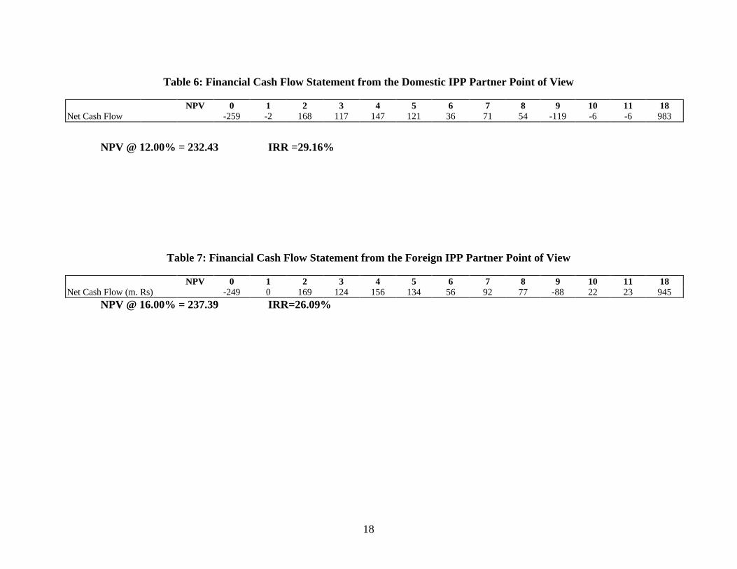
(ROR) is 29.16% (42.40% nominal) for the domestic IPP partner and 34.98% (39.03% nominal)
for the foreign partner. This positive NPV is due largely to the Special Appropriation and ROE
payments noted above.21 The financial NPV to the domestic IPP partner is 232.43 million rupees
(Table 6)22, and 237.39 million (US$3.02 million) rupees to the foreign IPP partner (Table 7).23
To the IPP, it is doubtlessly a profitable project as long as the PPA is honored by theutility.
21 See the Methodology section above.22 Using a real discount rate of 12%, Annex 25.23 Using a real discount rate of 16%, Annex 26.

16
Table 4: Financial Cash Flow from the Utility Point of View
(expressed in 1995 prices)
Year NPV 0 1 2 3 4 5 6 7 18Revenue* 911 1,847 1,847 1,847 1,847 1,847 1,847 0PV of Future Benefits 0 0 0 0 0 0 0 1,710
Bulk Power Cost 802 1,458 1,450 1,424 1,907 1,893 1,954 0Transfer Price 0 0 0 0 0 0 0 1,710Transmission, Distribution and Operating Cost 177 326 295 268 243 220 200 0Change In Working Capital 156 175 29 29 29 29 29 (288)
Net Cash flow (224) (112) 72 125 (333) (296) (336) 288
NPV @ 10.00% = (18.03) IRR = -4.63%

17
Table 5: Financial Real Cash Flow Statement from the IPP Point of View
(expressed in 1995 prices)
Year 0 1 2 3 4 5 6 7 18
ReceiptsSales - 801.52 1,457.78 1,449.90 1,423.97 1,907.31 1,893.08 1,953.79 - Change in Accounts Receivable - (63.87) (189.05) (122.17) (31.01) (28.17) (104.79) (36.37) 285.88 Transfer Price - - - - - - - - 1,710.01 Liquidation Values Land - - - - - - - - - Civil Work - - - - - - - - - Mechanical Work - - - - - - - - - Electrical Work - - - - - - - - - Other EPC - - - - - - - - - Other Investments - - - - - - - - - Loan 1,305.44 1,005.72 - - - - - - - Loan for Working Capital 52.06 234.97 344.35 343.04 338.71 419.27 416.90 427.02 - Total Inflows 1,357.50 1,978.34 1,613.07 1,670.77 1,731.68 2,298.41 2,205.19 2,344.44 1,995.89 ExpendituresInvestment Costs Land 6.60 - - - - - - - - EPC Cost Civil Works 70.70 - - - - - - - - Mechanical Works 1,027.66 1,027.66 - - - - - - - Electrical Works 44.54 44.54 - - - - - - - Miscellaneous 68.28 68.28 - - - - - - - Development Cost 136.00 - - - - - - - - Financial Charges 93.00 93.00 - - - - - - - Interest During Construction 289.44 142.56 - - - - - - - Pre-operative Expenses 50.00 - - - - - - - - Vehicle, Office, Apparatus 18.00 - - - - - - - - Contingency for EPC 60.70 60.70 - - - - - - - Cost Overrun - - - - - - - - -
Operation Costs Fixed Costs O & M Expenses - 35.08 70.16 70.16 70.16 70.16 70.16 70.16 - Salaries - 6.19 12.38 12.38 12.38 12.38 12.38 12.38 - Variable Costs Naphtha - 482.20 977.80 977.80 977.80 977.80 977.80 977.80 - Change in Accounts Payable - (40.18) (45.04) (7.58) (7.58) (7.58) (7.58) (7.58) 73.90 Change in Cash Balance - 3.44 3.76 0.64 0.64 0.64 0.64 0.64 (6.24) Loan Repayment Interest - - - - - 343.05 281.69 223.04 - Principal - - - - - 276.59 293.48 311.40 - Loan for Working Capital Interest - 9.66 43.61 63.91 63.67 62.87 77.82 77.38 - Principal - 47.22 213.12 312.32 311.13 307.21 380.27 378.12 - Income Tax - - - - - - 26.26 138.20 - Total Outflows 1,864.92 1,980.35 1,275.79 1,429.63 1,428.20 2,043.12 2,112.92 2,181.54 67.67 Net Cash Flow (507.42) (2.00) 337.28 241.13 303.48 255.29 92.27 162.89 1,928.23
NPV @ 13.96% = 476.09 IRR = 32.19%
18
Table 6: Financial Cash Flow Statement from the Domestic IPP Partner Point of View
NPV 0 1 2 3 4 5 6 7 8 9 10 11 18Net Cash Flow -259 -2 168 117 147 121 36 71 54 -119 -6 -6 983
NPV @ 12.00% = 232.43 IRR =29.16%
Table 7: Financial Cash Flow Statement from the Foreign IPP Partner Point of View
NPV 0 1 2 3 4 5 6 7 8 9 10 11 18Net Cash Flow (m. Rs) -249 0 169 124 156 134 56 92 77 -88 22 23 945
NPV @ 16.00% = 237.39 IRR=26.09%

19
VI. SENSITIVITY AND RISK ANALYSES OF FINANCIAL APPRAISAL
A. Sensitivity Analysis
A sensitivity analysis is conducted to determine the impact of changes in the key
variables on the financial NPVs of the project. Such a sensitivity analysis will tell if the project
can survive significant changes in variables like inflation, fuel prices and cost overruns, which
are not controlled by either party. A sensitivity analysis will also allow each party to know how
changes in those key variables that are to be negotiated through the Power Purchase Agreement
may influence the outcome of the project. Tables 8 through 25 show the effect of such changes
on the financial NPVs of the project.
The NPVs are calculated as of 1995 and expressed in terms of the 1995 price level.
Unless otherwise stated all NPV values reported below will be given in millions of rupees.
1. Selling Price of Electricity
Table 8: Effect Of Electricity Selling Price On The Financial NPV From The Utility's PointOf View
Average Real Electricity NPVSelling Price (million Rs)
2.4 (1,952)2.6 (985)2.8 (18)3.0 9493.1 1,4333.2 1,9163.3 2,4003.4 2,8843.5 3,3673.6 3,8513.7 4,334
Using a real discount rate of 10%, the utility will break even when the tariff to its
customers is set at 2.8037 Rs/kWh. At the present tariff of 2.8 Rs/kWh, the utility will lose
money on the deal.
20
2. Domestic Inflation
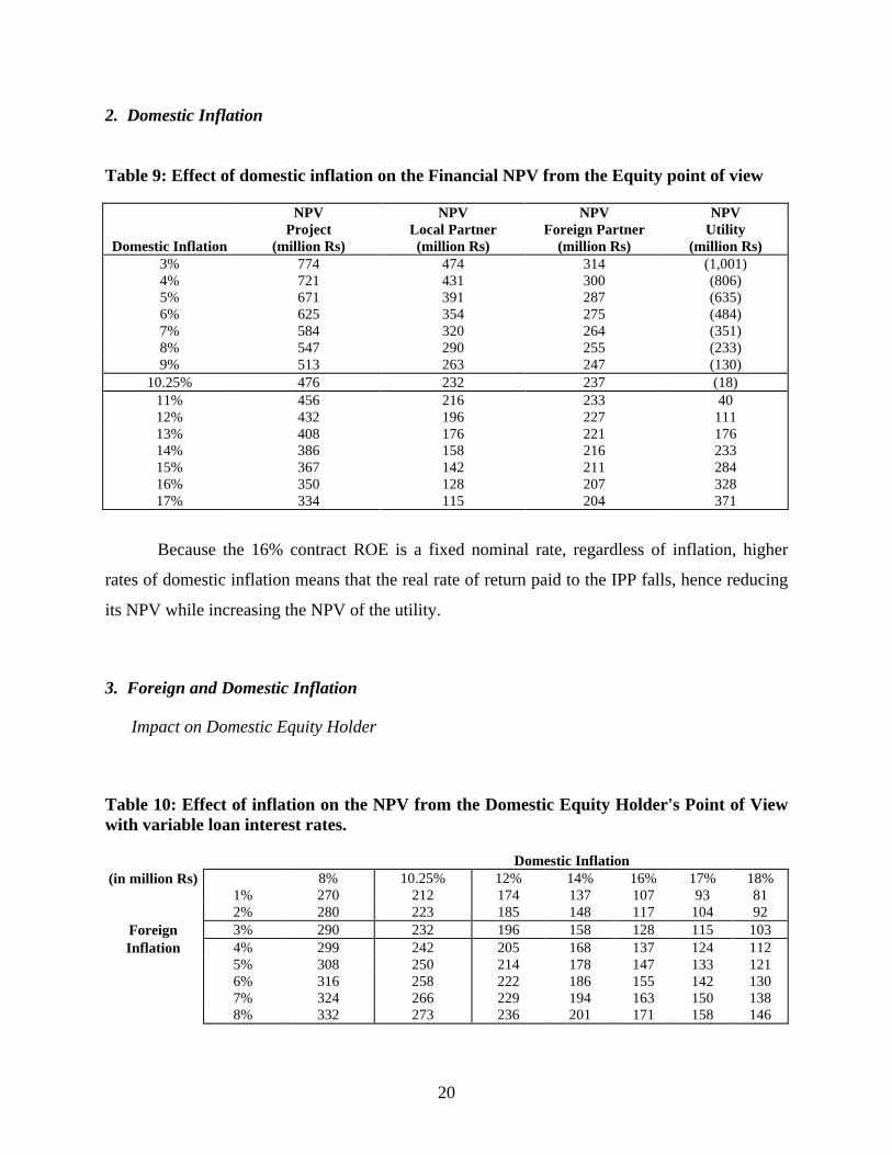
Table 9: Effect of domestic inflation on the Financial NPV from the Equity point of view
NPV NPV NPV NPVProject Local Partner Foreign Partner Utility
Domestic Inflation (million Rs) (million Rs) (million Rs) (million Rs)3% 774 474 314 (1,001)4% 721 431 300 (806)5% 671 391 287 (635)6% 625 354 275 (484)7% 584 320 264 (351)8% 547 290 255 (233)9% 513 263 247 (130)
10.25% 476 232 237 (18)11% 456 216 233 4012% 432 196 227 11113% 408 176 221 17614% 386 158 216 23315% 367 142 211 28416% 350 128 207 32817% 334 115 204 371
Because the 16% contract ROE is a fixed nominal rate, regardless of inflation, higher
rates of domestic inflation means that the real rate of return paid to the IPP falls, hence reducing
its NPV while increasing the NPV of the utility.
3. Foreign and Domestic Inflation
Impact on Domestic Equity Holder
Table 10: Effect of inflation on the NPV from the Domestic Equity Holder's Point of Viewwith variable loan interest rates.
Domestic Inflation(in million Rs) 8% 10.25% 12% 14% 16% 17% 18%
1% 270 212 174 137 107 93 812% 280 223 185 148 117 104 92
Foreign 3% 290 232 196 158 128 115 103Inflation 4% 299 242 205 168 137 124 112
5% 308 250 214 178 147 133 1216% 316 258 222 186 155 142 1307% 324 266 229 194 163 150 1388% 332 273 236 201 171 158 146

21
As mentioned above, higher domestic inflation leads to a smaller real fixed ROE payment
by the utility to the IPP causing both the IPP’s NPV as well as the domestic partner’s NPV to
fall. With an increase in foreign inflation, the value of the foreign loan decreases in rupee terms
because for the same domestic inflation there is less devaluation of the rupee. The IPP will have
less debt (principal) to repay relative to the amount of depreciation plus special appropriation
they receive. This will increase the domestic partner’s NPV. The decrease in foreign debt
repayment outflow due to a lower rate of devaluation of the rupee is partially offset by the
decrease in the "PPA Payment" by the utility to the IPP. In addition, the total "PPA Payment" is
reduced and the interest on foreign loans and the income tax components of the interest on the
contractual working capital decrease.
- In summary, the decrease in foreign principal payments (outflow) decreases the
amount of special appropriation (inflow), which causes the total "PPA Payment" to
decrease, thereby decreasing the interest expenses for working capital and income
taxes even further. However, the decrease in special appropriation (from the lower
rate of depreciation) is not enough to offset the lower principal payments. Therefore,
even though the inflows decrease, the outflows decrease even more, so the NPV
increases from the point of view of the domestic equity holder.
Impact on Foreign Equity Holder
Table 11: Effect of inflation on the NPV from the Foreign Equity Holder's Point of Viewwith variable loan interest rates.
Domestic Inflation(in million Rs) 4% 6% 8% 10.25% 12% 14% 16% 18%
1% 327 301 281 264 252 241 232 2262% 313 287 267 250 239 228 219 213
Foreign 3% 300 275 255 237 227 216 207 201Inflation 4% 289 264 244 226 216 205 196 190
5% 279 254 234 216 206 195 187 1816% 269 245 225 207 196 187 178 1727% 260 237 216 199 188 179 170 1648% 252 229 209 191 180 171 163 157

22
The foreign equity holder receives his return in US dollars. Higher domestic inflation
rates lower the real fixed ROE payment to the IPP, reducing the NPV values of both domestic
and foreign equity holders. A higher foreign inflation rate raises the value of rupees and lowers
the dollar value of the foreign partner’s rupee incomes, hence reducing his NPV as well.
Therefore, the foreign equity holder is affected negatively by an increase in the inflation rate of
either India or the US.
4. Fixed Nominal ROE of PPA
Table 12: Effect Of The Contract Nominal ROE On The IPP’s Financial NPV24
NPV NPV NPVContract Project Local Partner Foreign Partner
ROE (million Rs) (million Rs) (million Rs)7% 53 34 198% 100 56 449% 147 78 68
10% 194 100 9212% 288 144 14014% 382 188 18916% 476 232 23718% 570 277 28620% 664 321 334
The local partner will break even at 5.46% contract ROE; the foreign partner will break
even at 6.2%. The sensitivity analysis also shows that the higher the specified ROE in the contract
the higher the net present values of the project will be to each of the IPP owners.
24 Assumes an average 8% inflation in India and 3% foreign (US) inflation over the life of the project, the real
discount rate for the project is 13.96%, for the local partner 12%, and for the foreign partner 16%.

23
5. Real Discount Rate
Real Discount Rate’s Impact on Domestic Equity Holder
Table 13: Effect Of Real Discount Rate On The Financial NPV From The Domestic EquityHolder’s Point Of View
Nominal Real NPVDiscount Rate Discount Rate (million Rs)
21.28% 10.00% 29323.49% 12.00% 23225.69% 14.00% 18432.31% 20.00% 8637.82% 25.00% 3342.23% 29.00% 142.45% 29.20% 043.33% 30.00% -644.43% 31.00% -1345.54% 32.00% -19
The discount rates at which the domestic partners’ NPV becomes zero are the actual rates of
return on their equity. Assuming an 8% rate of inflation, the actual real ROE to the domestic equity
holder is 29.2% yielding a nominal return of 42.45%. Again, this shows that actual returns to the
equity holders can deviate greatly to the contract’s fixed ROE.
Real Discount Rate’s Impact on Foreign Equity Holder
Table 14: Effect Of Real Discount Rate On The Financial NPV From The Foreign EquityHolder’s Point Of View
Nominal Real NPV NPVDiscount Rate Discount Rate (million Rs) (million US$)
17.42% 14.00% 290 3.9019.48% 16.00% 237 3.0225.66% 22.00% 127 1.0226.69% 23.00% 113 0.7527.72% 24.00% 100 0.4928.75% 25.00% 88 0.2529.78% 26.00% 77 0.0230.81% 27.00% 66 (0.20)31.84% 28.00% 56 (0.41)
The actual real ROE to foreign equity holder is 26.0%. This implies a 29.78% nominal
ROE assuming a 3% rate of foreign inflation.
24
6. Incentive Points
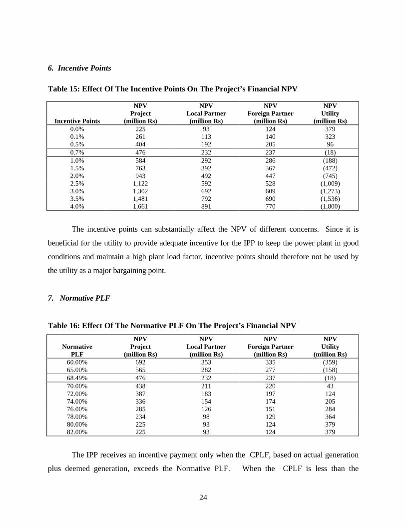
Table 15: Effect Of The Incentive Points On The Project’s Financial NPV
NPV NPV NPV NPVProject Local Partner Foreign Partner Utility
Incentive Points (million Rs) (million Rs) (million Rs) (million Rs)0.0% 225 93 124 3790.1% 261 113 140 3230.5% 404 192 205 960.7% 476 232 237 (18)1.0% 584 292 286 (188)1.5% 763 392 367 (472)2.0% 943 492 447 (745)2.5% 1,122 592 528 (1,009)3.0% 1,302 692 609 (1,273)3.5% 1,481 792 690 (1,536)4.0% 1,661 891 770 (1,800)
The incentive points can substantially affect the NPV of different concerns. Since it is
beneficial for the utility to provide adequate incentive for the IPP to keep the power plant in good
conditions and maintain a high plant load factor, incentive points should therefore not be used by
the utility as a major bargaining point.
7. Normative PLF
Table 16: Effect Of The Normative PLF On The Project’s Financial NPV
NPV NPV NPV NPVNormative Project Local Partner Foreign Partner Utility
PLF (million Rs) (million Rs) (million Rs) (million Rs)60.00% 692 353 335 (359)65.00% 565 282 277 (158)68.49% 476 232 237 (18)70.00% 438 211 220 4372.00% 387 183 197 12474.00% 336 154 174 20576.00% 285 126 151 28478.00% 234 98 129 36480.00% 225 93 124 37982.00% 225 93 124 379
The IPP receives an incentive payment only when the CPLF, based on actual generation
plus deemed generation, exceeds the Normative PLF. When the CPLF is less than the
25
Normative PLF, assuming IPP bears the responsibility, the fixed charge payment to the IPP will
be reduced proportionally. This explains why the project’s and the IPP partners’ break even
points are quite sensitive to the Normative PLF.
8. Actual Plant Load Factor
Impact on the IPP’s NPV
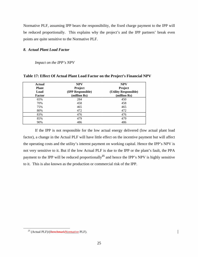
Table 17: Effect Of Actual Plant Load Factor on the Project’s Financial NPV
Actual NPV NPVPlant Project ProjectLoad (IPP Responsible) (Utility Responsible)
Factor (million Rs) (million Rs)65% 284 45070% 458 45875% 465 46580% 472 47283% 476 47685% 479 47990% 486 486
If the IPP is not responsible for the low actual energy delivered (low actual plant load
factor), a change in the Actual PLF will have little effect on the incentive payment but will affect
the operating costs and the utility’s interest payment on working capital. Hence the IPP’s NPV is
not very sensitive to it. But if the low Actual PLF is due to the IPP or the plant’s fault, the PPA
payment to the IPP will be reduced proportionally25 and hence the IPP’s NPV is highly sensitive
to it. This is also known as the production or commercial risk of the IPP.
25 (Actual PLF)/(BenchmarkNormative PLF).

26
Impact on The Utility’s NPV
Table 18: Effect Of Actual Plant Load Factor on the Utility’s Financial NPV
Actual NPV NPVPlant Utility UtilityLoad (IPP Responsible) (Utility Responsible)
Factor (million Rs) (million Rs)65% (588) (869)70% (633) (633)75% (396) (396)80% (160) (160)83% (18) (18)85% 77 7790% 313 313
If the lower Actual PLF is due to the utility’s failure to take the power, it is very
detrimental to the utility who must pay for the plant. This is the demand risk of the utility. But if
the low Actual PLF is due to the IPP or the plant’s fault, the PPA’s fixed charge payment as well
as the variable charge payment to the IPP will be reduced proportionally, hence the utility’s
financial loss is actually reduced. On the other hand, if the utility’s tariff is high enough such that
the utility has a positive NPV, the situation will be reversed - the utility’s NPV decreases as the
Actual PLF declines.
Impact on the Utility’s Break Even Tariff
Table 19: Actual Plant Load Factor and the Utility’s Break Even Tariff
Tariff (Net of Tax)2.8 2.9 3.0 3.1 3.2
70% (633) (225) 183 591 999Actual Plant 75% (396) 41 478 915 1,352Load Factor 80% (160) 306 772 1,239 1,705
83% (18) 466 949 1,433 1,91685% 77 572 1,067 1,562 2,05890% 313 837 1,362 1,886 2,41095% 549 1,103 1,656 2,210 2,763
If the Actual PLF is 83%, the utility needs a 2.8037 Rs/kWh tariff to break even. As the
Actual PLF becomes higher, the break-even tariff gets lower. Given the Actual PLF, the utility’s
financial position depends ultimately on the utility’s tariff policy.

27
9. Residual Value Ratio
Table 20: Effect Of The Residual Value Ratio On The Project’s Financial NPV
NPV NPV NPV NPVResidual Value Project Local Partner Foreign Partner Utility
Ratio (million Rs) (million Rs) (million Rs) (million Rs)0.0 549 273 270 (134)0.1 476 232 237 (18)0.2 399 190 203 1040.3 318 144 166 2330.4 236 99 130 3610.5 145 48 89 5020.6 52 (3) 47 6450.7 (50) (59) 1 801
The [(1-Residual Value Ratio) * (Investment Cost) ] value decides the total amount of
depreciation and special appropriation payments. The higher the (1-Residual Value Ratio) value
(or the lower the Residual Value Ratio) the higher the total amount of depreciation and special
appropriation payments. The Residual Value Ratio therefore strongly affects the rate of return
to the project and the IPP partners.26
10. Cost Overruns
Table 21: Effect Of Cost Overrun On The Project’s Financial NPV
NPV Project NPV Project NPV Utility NPV UtilityCost IPP Utility IPP Utility
Overrun Responsible Responsible Responsible Responsible-20% 806 (187) (18) 713-10% 641 144 (18) 3490% 476 476 (18) (18)
10% 311 808 (18) (384)20% 146 1,139 (18) (749)30% (18) 1,471 (18) (1,106)40% (183) 1,803 (18) (1,454)50% (348) 2,134 (18) (1,803)
26 This ratio is more reasonable if it is set to near the {1-(project life/economic life) } value so that the real
present value of the undepreciated book value of the investment is closer to the real transfer price of the plant,assuming that the real transfer price will be close to the residual value estimated by {(economic life – projectlife)/economic life}*initial investment cost.
28
If the IPP is responsible for cost overruns, cost overruns will have a significant negative
effect on the IPP’s NPV. If the utility is to bear the cost overruns, the greater the cost overruns,
the higher the IPP’s NPV will be. Because of the “fixed-return” nature of the PPA, a higher-
capital-cost project tends to benefit the IPP. This also tends to provide an incentive for the IPP
to have a more capital intensive project. This fact is also reflected in the utility’s NPV which
worsens as cost overruns are heightened. The responsibility for cost overruns is therefore one of
the critical elements in a fixed-ROE type PPA.
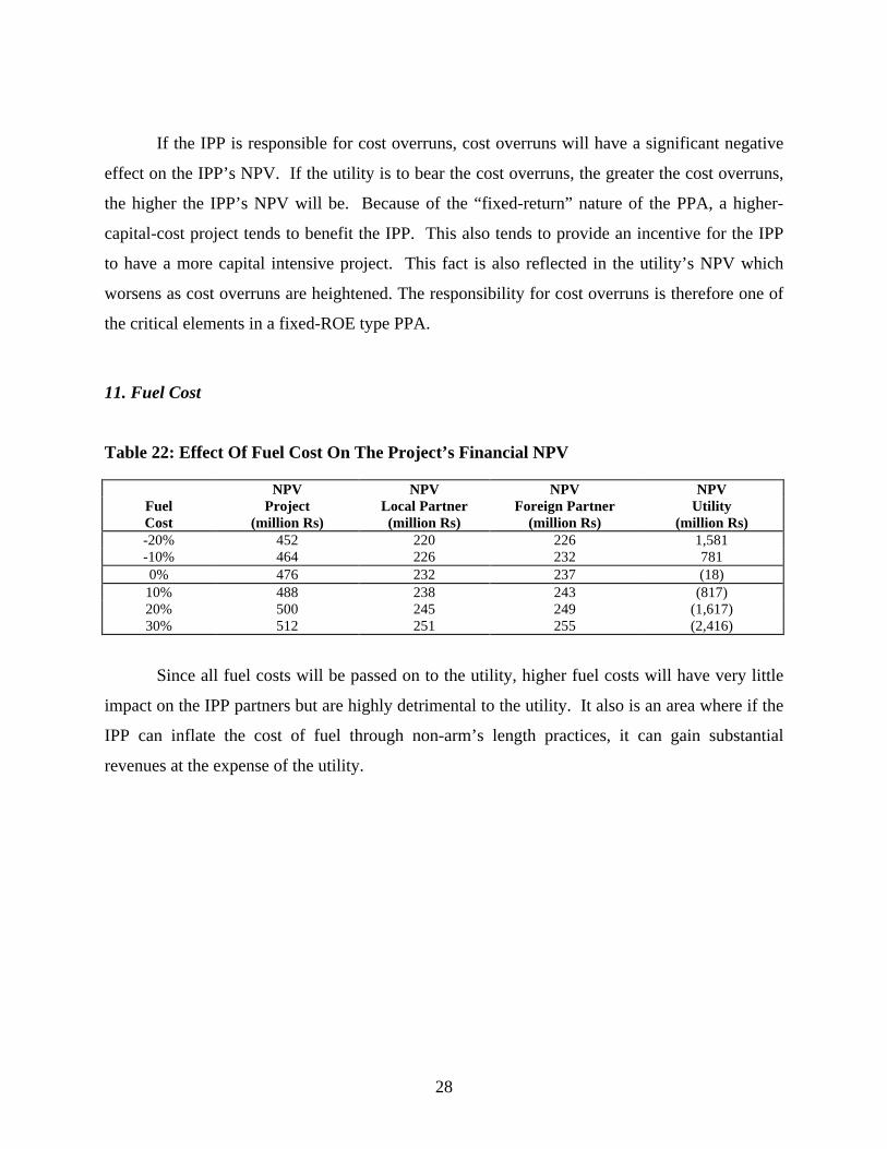
11. Fuel Cost
Table 22: Effect Of Fuel Cost On The Project’s Financial NPV
NPV NPV NPV NPVFuel Project Local Partner Foreign Partner UtilityCost (million Rs) (million Rs) (million Rs) (million Rs)-20% 452 220 226 1,581-10% 464 226 232 7810% 476 232 237 (18)
10% 488 238 243 (817)20% 500 245 249 (1,617)30% 512 251 255 (2,416)
Since all fuel costs will be passed on to the utility, higher fuel costs will have very little
impact on the IPP partners but are highly detrimental to the utility. It also is an area where if the
IPP can inflate the cost of fuel through non-arm’s length practices, it can gain substantial
revenues at the expense of the utility.

29
12. Actual Fuel Cost Factor
Table 23: Effect of IPP's Actual Fuel Cost Factor on the Project Financial NPV
NPV NPV NPV NPVFuel Project Local Partner Foreign Partner UtilityCost (million Rs) (million Rs) (million Rs) (million Rs)80% 1,638 897 746 (18)90% 1,057 565 492 (18)
100% 476 232 237 (18)110% (105) (100) (17) (18)120% (686) (433) (272) (18)130% (1,267) (765) (526) (18)
The PPA’s variable charge payments are fixed in terms of electricity heat rate and fuel
calorific value specified in the PPA. If the IPP can manage to achieve lower heat rate or higher
fuel calorific value or both, it can save on the fuel costs, while the utility continues to pay the
contract amount based on the predefined heat rate and calorific value. Lower actual fuel costs
(relative to the contract fuel costs) will greatly benefit the IPP but not the utility. A better
formulation of the fuel cost formula is to include an incentive for the IPP to lower the fuel costs
and a mechanism to pass on part of the savings to the utility.
13. Real Loan Rates
Real Loan Rates’ Impact on the IPP
Table 24: Effect of Real Loan Rates on the Project’s Financial NPV From Equity Holder’sPoint of View (in million Rs)
Real Domestic Debt Interest Rate5.0% 6.5% 8.0% 10.0% 12.0%
3.0% 506 493 479 460 4374.0% 499 486 472 453 430
Real Foreign Debt 5.3% 489 476 462 443 420Interest Rate 6.0% 484 471 457 438 415
7.0% 467 454 440 421 3988.0% 459 446 433 413 3909.0% 461 448 434 415 392
Because interest during the grace period is accrued to the principal, an increase in the real
rate of interest on both the domestic and the foreign loan rate will increase the total loan

30
principal to be repaid. The increase in interest payments will be automatically compensated for
by changes in the PPA payment paid to the IPP, since these are part of the fixed charge payment.
The increase in principal repayments will cause the special appropriation to be higher in the
earlier years, but lower in the later years because this payment is limited to the point when the
IPP recovers its initial investment. Therefore, the net present value of the special appropriation
will be higher. However, this increase in special appropriation is not enough to compensate for
the increase in the present value of the principal repayments. As a result, an increase in the real
interest rate on any of the loans will reduce the project’s financial NPV.
Real Loan Rates’ Impact on the Utility
Table 25: Effect of Real Loan Rates on the Project’s Financial NPV From Utility’s Point ofView (in million Rs)
Real Domestic Debt Interest Rate5.0% 6.5% 8.0% 10.0% 12.0%
3.0% 153 93 25 (71) (175)4.0% 108 48 (20) (116) (220)
Real Foreign Debt 5.3% 43 (18) (85) (182) (285)Interest Rate 6.0% 8 (53) (120) (217) (320)
7.0% (24) (84) (152) (248) (352)8.0% (84) (144) (211) (308) (411)9.0% (172) (233) (300) (397) (500)
10.0% (216) (276) (344) (440) (544)
From the utility’s point of view, a power purchase agreement can be treated either as a
simple bulk power purchase from an outside IPP or as a financing deal. For a fixed-ROE type
PPA (vis-à-vis a fixed kWh price PPA), it is more representative to take the latter view. As a
financing deal, both the true rate of return on equity and the loan rates are important. As shown
in Table 24, the real domestic loan rate has a smaller impact on the project NPV from the equity
holder’s point of view because the loan interest is paid by the utility.27 In contrast, higher loan
rates, both domestic and foreign, cause the utility’s NPV to deteriorate substantially (Table 25).
27 The small impact from real foreign loan rate is deal to the slow increase in real exchange rate.

31
B. Conclusions – Sensitivity Analysis
The sensitivity analysis based on such a financial model allows us to evaluate the relative
impact of each of the variables contained in a power purchase agreement. It is clear that the
actual plant load factor is a key variable from the point of view of the utility. If it falls, and it is
the utility’s responsibility, it will cause the NPV of the utility to fall dramatically. It also is very
costly to the IPP if it is the party responsible for the low plant factor. Depending on whose
responsibility is the cost overruns, they can have serious impact on either parties’ NPV. The
fixed nominal ROE of the PPA (the contract ROE) can substantially affect the final NPVs, even
though it does not exclusively determine the actual rate of return to the IPP. The actual fuel costs
of the plant and the real exchange rate are risk variables outside the control of the utility. They
can nevertheless have an important impact on the utility when it undertakes this project with this
type of PPA.
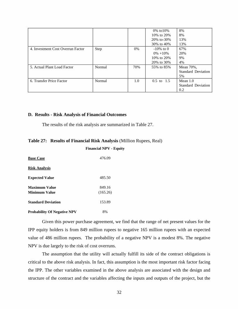
C. Risk Analysis
The assumptions and probability distributions for the various risk variables used in the
risk analysis are summarized in Table 26. Details of these assumptions are given in Appendix I.
Table 26: Specification of Risk Variables
Risk Variable Probability
Distribution
Base
Case
Value
Range Value Probability
1. Inflation Rate Disturbance Step (Independent
Yearly)
0% -(50-100%)-(30-50%)-(10-30%)-(0-10%)0-10%
10-30%30-50%
50-100%
14%14%10%12%12%10%14%14%
2. Real Exchange Rate Disturbance Step (Independent,
yearly)
0% -20% to -10%0% to -10%0% to 10%
10% to 20%20% to 30%30% to 50%
30%32%10%15%12%1%
3. Annual Fuel Cost Disturbance Normal
(Independent,
yearly)
0% -40% to -30%-30% to -20%-20% to -10%-10% to 0%%
4%13%25%16%
32
0% to10%10% to 20%20% to-30%30% to 40%
8%8%13%13%
4. Investment Cost Overrun Factor Step 0% -10% to 00% +10%
10% to 20%20% to 30%
67%20%9%4%
5. Actual Plant Load Factor Normal 70% 55% to 85% Mean 70%,Standard Deviation5%
6. Transfer Price Factor Normal 1.0 0.5 to 1.5 Mean 1.0Standard Deviation0.2
D. Results - Risk Analysis of Financial Outcomes
The results of the risk analysis are summarized in Table 27.
Table 27: Results of Financial Risk Analysis (Million Rupees, Real)
Financial NPV - Equity
Base Case 476.09
Risk Analysis
Expected Value 485.50
Maximum Value 849.16Minimum Value (165.26)
Standard Deviation 153.89
Probability Of Negative NPV 8%
Given this power purchase agreement, we find that the range of net present values for the
IPP equity holders is from 849 million rupees to negative 165 million rupees with an expected
value of 486 million rupees. The probability of a negative NPV is a modest 8%. The negative
NPV is due largely to the risk of cost overruns.
The assumption that the utility will actually fulfill its side of the contract obligations is
critical to the above risk analysis. In fact, this assumption is the most important risk factor facing
the IPP. The other variables examined in the above analysis are associated with the design and
structure of the contract and the variables affecting the inputs and outputs of the project, but the
33
political and financial ability of the utility to deliver on its commitments can not be modeled in
the same manner.
VII. ECONOMIC ANALYSIS
A power project providing shortage power will have an impact on the consumers directly
affected by the power shortages and indirectly on the state economy by eliminating the
deterrence to potential domestic and foreign investment in the state. We shall refer to the
potential demand for electricity in the state discouraged by the power shortages as the “deterred
demand”.
A. Methodology
Value Of Electricity With Power Shortages
When a power shortage situation arises and persists for some time, some firms and
residential customers may decide to install their own generators. Some would decide to conduct
their business without electricity while others may simply cut back some of their activities that
require electricity. Furthermore, some firms which otherwise would have located in the country
or state may decide not to come. We shall refer to the potential demand for electricity in the
state discouraged by the power shortages as the “deterred demand”.
The direct benefits of providing electricity to the customers are measured by their
willingness to pay for the power. In addition to the direct benefits accruing as a result of
elimination of power shortages to those affected customers, there will be the added benefits due
to reduction in the deterred demand. Because of the lack of a good measure of the quantity of
deterred demand, these benefits are not included in this study. They nevertheless are an
important consideration.
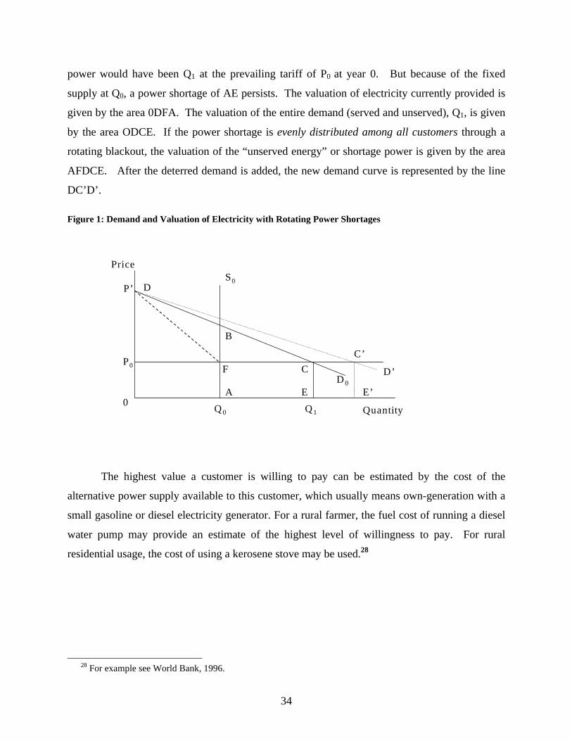
In Figure 1, the supply of power by the existing system is fixed at the level Q0 in year 0,
represented by the vertical supply curve, Q0S0. Based on the demand curve DD0, the demand for
34
power would have been Q1 at the prevailing tariff of P0 at year 0. But because of the fixed
supply at Q0, a power shortage of AE persists. The valuation of electricity currently provided is
given by the area 0DFA. The valuation of the entire demand (served and unserved), Q1, is given
by the area ODCE. If the power shortage is evenly distributed among all customers through a
rotating blackout, the valuation of the “unserved energy” or shortage power is given by the area
AFDCE. After the deterred demand is added, the new demand curve is represented by the line
DC’D’.
Figure 1: Demand and Valuation of Electricity with Rotating Power Shortages
0
P0
P’ D
F
A
C
E E’D 0
D’
C’
S0
Q 0
B
Q 1 Quantity
Price
The highest value a customer is willing to pay can be estimated by the cost of the
alternative power supply available to this customer, which usually means own-generation with a
small gasoline or diesel electricity generator. For a rural farmer, the fuel cost of running a diesel
water pump may provide an estimate of the highest level of willingness to pay. For rural
residential usage, the cost of using a kerosene stove may be used.28
28 For example see World Bank, 1996.
35
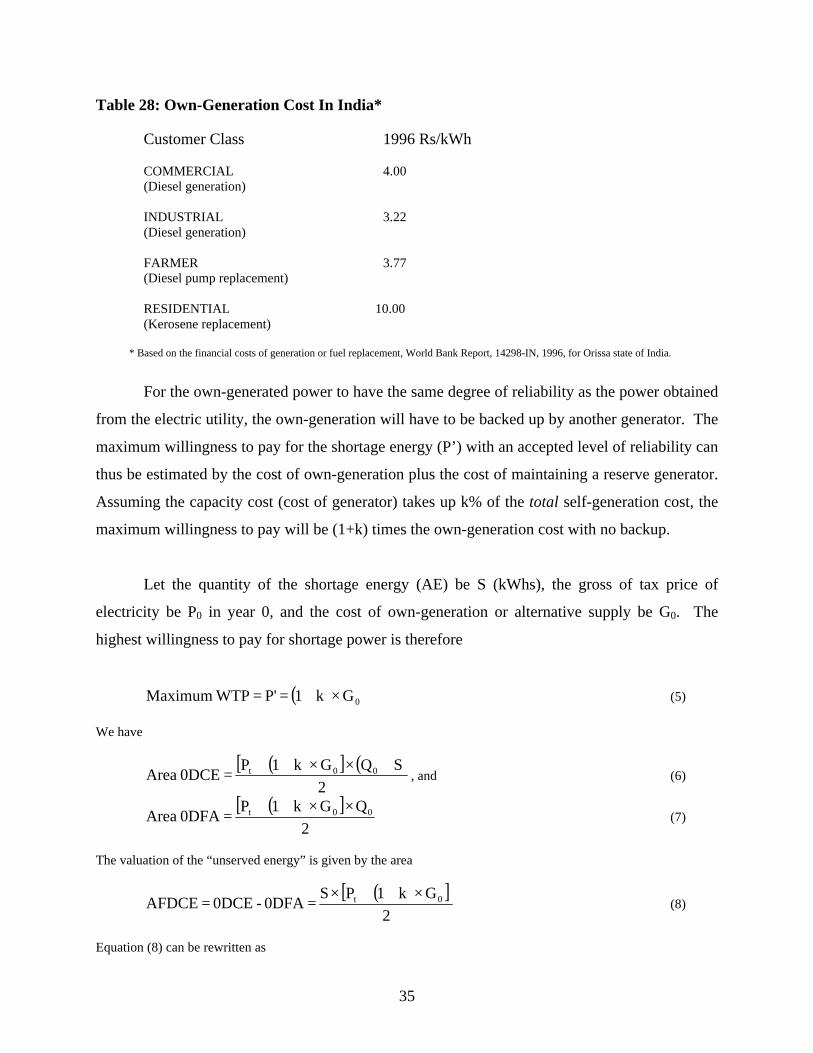
Table 28: Own-Generation Cost In India*
Customer Class 1996 Rs/kWh
COMMERCIAL 4.00(Diesel generation)
INDUSTRIAL 3.22(Diesel generation)
FARMER 3.77(Diesel pump replacement)
RESIDENTIAL 10.00(Kerosene replacement)
* Based on the financial costs of generation or fuel replacement, World Bank Report, 14298-IN, 1996, for Orissa state of India.
For the own-generated power to have the same degree of reliability as the power obtained
from the electric utility, the own-generation will have to be backed up by another generator. The
maximum willingness to pay for the shortage energy (P’) with an accepted level of reliability can
thus be estimated by the cost of own-generation plus the cost of maintaining a reserve generator.
Assuming the capacity cost (cost of generator) takes up k% of the total self-generation cost, the
maximum willingness to pay will be (1+k) times the own-generation cost with no backup.
Let the quantity of the shortage energy (AE) be S (kWhs), the gross of tax price of
electricity be P0 in year 0, and the cost of own-generation or alternative supply be G0. The
highest willingness to pay for shortage power is therefore
( ) 0G k 1 P' WTPMaximum ×+== (5)
We have
( )[ ] ( )2
S Q G k 1 P 0DCE Area 00t +××++
= , and (6)
( )[ ]2
Q G k 1 P 0DFA Area 00t ××++
= (7)
The valuation of the “unserved energy” is given by the area
( )[ ]2
G k 1 P S 0DFA - 0DCE AFDCE 0t ×++×
== (8)
Equation (8) can be rewritten as

36
( )[ ]2
G k 1 P S S WTP 0t
s
×++×=× (9)
where WTPS is the average willingness to pay per unit of shortage power, S is the quantity of
shortage power, Pt is the prevailing gross of tax price of electricity in year t, P0 is the gross of
tax price of electricity in year 0 when the alternative power cost is estimated or power price at
the beginning of the project, k is the capacity cost as a percentage of the alternative power supply
cost, and G0 is an estimation of the alternative power cost.
From equation (9), the average willingness to pay per unit of shortage power is given by the
maximum willingness to pay plus the prevailing tariff in year t divided by 2, or
2
P' P WTPAverage t +
= (10)
For this study, the calculation of the average willingness to pay is given in Table 29.
Table 29: Own-Generation Costs, Average Tariff, and Willingness To Pay in India (1996Prices)
Own-generation Cost (Rs/kWh) 3.500Average Power Price (Gross of Tax, Rs/kWh) 2.912Capacity Cost as Share of Total Generation Cost* (k) 0.258Maximum Willingness To Pay (Rs/kWh) 4.404Average Willingness To Pay in Year 0 (Rs/kWh) 3.658
It is important to note that the maximum willingness to pay will not be affected by the
changes in electricity tariffs over time. For this study, the maximum real willingness to pay is
assumed to stay constant in real terms at its year 0 (1996 in this case) level. The average
willingness to pay for each year of the project is calculated as the average of the maximum
willingness to pay and the prevailing real tariff.

37
B. Project Benefits and Costs
The statements of economic benefits and costs for the project are shown in Table 30. The
economic cost of capital for India used to discount the statements of economic benefits and costs
is estimated to be 10.86%.
C. Results
The economic appraisal of the SPPL project is based on the total investment real cash
flow from the IPP point of view adjusted for the economic costs and values of all the items and
discounted at the economic discount rate.
The economic NPV of the project is 5,042 million Rs. It should be noted that the
incremental economic NPV for the project is understated as the benefits from the elimination of
the deterred demand are not included.

38
Table 30: Economic Cash Flow Statement
Year CF 0 1 2 3 4 5 6 7 8 9 10 11 12 13 14 15 16 17 18NPV
ReceiptsSales 17,242 0 1,189 2,410 2,410 2,410 2,410 2,410 2,410 2,410 2,410 2,410 2,410 2,410 2,410 2,410 2,410 2,410 2,410 0Change in AccountsReceivable
(439) 1.000 0 (64) (189) (122) (31) (28) (105) (36) (47) (38) 9 (4) (29) (30) (30) (29) (28) (17) 286
Transfer Price 267 1.000 0 0 0 0 0 0 0 0 0 0 0 0 0 0 0 0 0 0 1,710Liquidation Values 0 0 0 0 0 0 0 0 0 0 0 0 0 0 0 0 0 0 0 0 Land 0 1.000 0 0 0 0 0 0 0 0 0 0 0 0 0 0 0 0 0 0 0 Civil Work 0 0.836 0 0 0 0 0 0 0 0 0 0 0 0 0 0 0 0 0 0 0 Mechanical Work 0 0.900 0 0 0 0 0 0 0 0 0 0 0 0 0 0 0 0 0 0 0 Electrical Work 0 0.900 0 0 0 0 0 0 0 0 0 0 0 0 0 0 0 0 0 0 0 Other EPC 0 1.000 0 0 0 0 0 0 0 0 0 0 0 0 0 0 0 0 0 0 0 Other Investments 0 1.000 0 0 0 0 0 0 0 0 0 0 0 0 0 0 0 0 0 0 0Total Inflows 17,070 0 1,125 2,221 2,288 2,379 2,382 2,305 2,374 2,363 2,372 2,419 2,406 2,381 2,380 2,380 2,381 2,382 2,393 1,996ExpendituresInvestment Costs Land 7 1.000 7 0 0 0 0 0 0 0 0 0 0 0 0 0 0 0 0 0 0 EPC Cost Civil Works 59 0.836 59 0 0 0 0 0 0 0 0 0 0 0 0 0 0 0 0 0 0 Mechanical Works 1,759 0.900 925 925 0 0 0 0 0 0 0 0 0 0 0 0 0 0 0 0 0 Electrical Works 76 0.900 40 40 0 0 0 0 0 0 0 0 0 0 0 0 0 0 0 0 0 Miscellaneous 117 0.900 61 61 0 0 0 0 0 0 0 0 0 0 0 0 0 0 0 0 0 Development Cost 136 1.000 136 0 0 0 0 0 0 0 0 0 0 0 0 0 0 0 0 0 0 Financial Charges Pre-operative Expenses 45 0.900 45 0 0 0 0 0 0 0 0 0 0 0 0 0 0 0 0 0 0 Vehicle, Office, Apparatus 16 0.900 16 0 0 0 0 0 0 0 0 0 0 0 0 0 0 0 0 0 0 Contingency for EPC 104 0.900 55 55 0 0 0 0 0 0 0 0 0 0 0 0 0 0 0 0 0Cost Overrun 0 1.000 0 0 0 0 0 0 0 0 0 0 0 0 0 0 0 0 0 0 0
Operation Costs Fixed Costs O & M Expenses 433 0.861 0 30 60 60 60 60 60 60 60 60 60 60 60 60 60 60 60 60 0 Salaries 85 0.955 0 6 12 12 12 12 12 12 12 12 12 12 12 12 12 12 12 12 0 Variable Costs Naphtha 6,711 0.959 0 463 938 938 938 938 938 938 938 938 938 938 938 938 938 938 938 938 0Change in Accounts Payable (106) 1.000 0 (40) (45) (8) (8) (8) (8) (8) (8) (8) (8) (8) (8) (8) (8) (8) (8) (8) 74Change in Cash Balance 9 1.000 0 3 4 1 1 1 1 1 1 1 1 1 1 1 1 1 1 1 (6)Income Tax 0 0.000 0 0 0 0 0 0 0 0 0 0 0 0 0 0 0 0 0 0 0Transmission & DistributionCosts
2,578 0.911 0 178 360 360 360 360 360 360 360 360 360 360 360 360 360 360 360 360 0
Total Outflows 12,028 1,344 1,720 1,329 1,364 1,364 1,364 1,364 1,364 1,364 1,364 1,364 1,364 1,364 1,364 1,364 1,364 1,364 1,364 68Net Cash Flow 5,042 (1,344) (596) 892 924 1,015 1,018 942 1,010 999 1,009 1,055 1,042 1,018 1,017 1,017 1,018 1,018 1,030 1,928
Economic NPV @ EOCK 10.86% = 5,042 Financial NPV @ EOCK = 418

39
VIII. SENSITIVITY AND RISK ANALYSES OF ECONOMIC APPRAISAL
A. Sensitivity Analysis
A sensitivity analysis is conducted on the economic NPV of the project. The variables
tested are similar to those for the financial sensitivity analysis except for those contract items that
would not affect the economic value of the project. The sensitivity of the economic NPV to the
own-generated power cost is added . The results of the sensitivity analysis are given below.
1. Domestic Inflation
Table 31: Effect Of Domestic Inflation On The Project’s Economic NPV
NPVEconomic
Domestic Inflation (million Rs)6% 3,3108% 4,046
10.25% 5,04212% 5,96214% 7,21016% 8,70918% 10,516
A higher rate of domestic inflation will increase the economic NPV only slightly.
2. Real Exchange Rate
Real Exchange Rate’s Impact on Economic NPV
Table 32: Effect Of Average Real Exchange Rate On Economic NPV
Appreciation / NPVDepreciation Economic
Factor (million Rs)80% 6,69390% 5,867
100% 5,042110% 4,217120% 3,392130% 2,567

40
The economic NPV is highly sensitive to real exchange rate. A real devaluation of the
exchange rate will cause the economic NPV to fall because of the greater cost of fuel (naphtha)
price, which is based on the import price of fuel, and the higher repayment of the foreign loans.
3. Fuel Cost
Table 33: Effect Of Fuel Cost On The Project’s Economic NPV
NPVFuel EconomicCost (million Rs)-20% 6,433-10% 5,7370% 5,042
10% 4,34720% 3,65230% 2,957
Economic NPV is quite sensitive to fuel costs: the higher the real fuel cost the lower is
the economic NPV.
4. Cost Overruns
Table 34: Effect Of Cost Overrun On The Project’s Economic NPV
NPVCost Project
Overrun (million Rs)-20% 5,375-10% 5,2090% 5,042
10% 4,87620% 4,70930% 4,543

41
The economic NPV is sensitive to cost overruns but the likely cost overruns will be small
relative to the size of the economic NPV.
5. Actual Plant Load Factor
Table 35: Effect Of Actual Plant Load Factor on the Project’s Economic NPV
NPV NPVEconomic Economic
Actual Plant (IPP Responsible) (Utility Responsible)Load Factor (million Rs) (million Rs)
40% 1,091 1,04750% 2,007 1,97660% 2,920 2,90570% 3,834 3,83483% 5,042 5,04290% 5,693 5,693
100% 6,622 6,622
The economic NPV is very sensitive to Actual Plant Load Factor but remains in the
positive range. This is because the economic value of the electricity of the project is high
relative to the cost of the project.
6. Own-Generation Cost
Table 36: Effect Of Own-Generation Cost Factor On The Project’s Economic NPV
Own-Generation NPVCost Factor Economic
(million Rs)0.800 1,5851.000 3,3141.200 5,0421.400 6,7711.600 8,5001.800 10,228
The economic NPV is very sensitive to the own-generation cost factor29, which
determines the maximum willingness to pay for electricity. The lower the own-generation cost
factor means the lower is the willingness to pay for power and hence the lower is the economic
29 The own-generation cost factor is defined as a multiplier of the own-generation cost for use in the sensitivity
analysis.

42
NPV. However, the economic NPV remains within the positive range despite the wide range of
the own-generation cost factor values.
B. Risk Analysis
Risk analysis was also applied to test how the economic return of the project responds to
possible changes in inflation, exchange rate, fuel cost, cost overruns, actual plant load factor, and
own-generation cost. The range limits and probability distributions of the risk variables are
shown in Table 37.

43
Table 37: Range Values and Probability Distributions of Risk Variables
Risk Variable Probability
Distribution
Base Case
Value
Range Value Probability
1. Inflation Rate Disturbance Step
(Independent
Yearly)
0% -(50-100%)-(30-50%)-(10-30%)-(0-10%)
0-10%10-30%30-50%
50-100%
14%14%10%12%12%10%14%14%
2. Real Exchange Rate
Disturbance
Step
(Independent,
yearly)
0% -20% to -10%0% to -10%0% to 10%
10% to 20%20% to 30%30% to 50%
30%32%10%15%12%1%
3. Annual Fuel Cost Disturbance Normal
(Independent,
yearly)
0% -40% to -30%-30% to -20%-20% to -10%-10% to 0%%
0% to10%10% to 20%20% to-30%30% to 40%
4%13%25%16%8%8%13%13%
4. Investment Cost Overrun
Factor
Step 0% -10% to 00% +10%
10% to 20%20% to 30%
67%20%9%4%
5. Actual Plant Load Factor Normal 70% 55% to 85% Mean 70%,
Standard Deviation 5%
6. Own-Generation Cost Normal 0% -25% to 25% Mean 0,
Standard Deviation 5%
Own-Generation Cost
The economic value of shortage power depends on the estimate of own-generation cost of
the cost of alternative power supply. The own-generation cost factor is used to adjust the own-
generation cost up or down within a range of plus and minus 25% from its base-case value. A
normal distribution with a mean of zero and a standard deviation of 5% is assumed for the own-
generation cost.
44
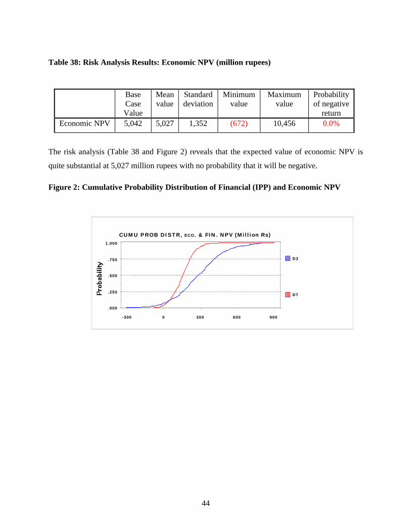
Table 38: Risk Analysis Results: Economic NPV (million rupees)
BaseCaseValue
Meanvalue
Standarddeviation
Minimumvalue
Maximumvalue
Probabilityof negative
returnEconomic NPV 5,042 5,027 1,352 (672) 10,456 0.0%
The risk analysis (Table 38 and Figure 2) reveals that the expected value of economic NPV is
quite substantial at 5,027 million rupees with no probability that it will be negative.
Figure 2: Cumulative Probability Distribution of Financial (IPP) and Economic NPV
CUMU PROB DISTR, ECO . & FIN. NPV (Million Rs)
.000
.250
.500
.750
1.000
-300 0 300 600 900
D3
D7
45
IX. STAKEHOLDER ANALYSIS
A project generates externalities when its economic benefits and costs are different from
its respective financial flows. The purpose of distributive analysis is to establish who is gaining
or loosing from the implementation of the project.
The steps followed in distributive analysis are:
i) identification of externalities item by item by subtracting the financial from theeconomic flows,
ii) reduction of each item’s flow of externality into a single figure by computing the netpresent value of each stream at the economic discount rate,
iii) allocation of externalities to various affected stakeholder groups in the economy.
A. Distribution of Externalities
The net present value, at the economic cost of capital, of the externalities generated by
the project amounts to 7,202 million rupees. The analysis of the allocation of externalities,
presented in Table 39, shows that the electricity consumers, government, IPP partners and
workers would gain if the project were implemented. The utility would be the only loser in this
project.
Table 39: Distribution Of Externalities
NPV (million Rs)Government 1,192Consumers 5,931Utility (69)IPP Domestic Partner 265IPP Foreign Partner 398Workers 78Total 7,796
The electricity consumers would gain 5,931 million rupees which is a measurement of the
willingness to pay by the consumers less the gross of tax power prices. The government would
46
have a positive externality of about 1,192 million rupees due mainly to the taxes and duties on
imported equipment and fuel. The workers would have a modest externality gain of 78 million
rupees because of their employment by the project. The utility would lose 69 million rupees due
to its “below-cost” tariff policy. The domestic partner of the IPP would gain 265 million rupees
while the foreign partner would gain 398 million rupees.30
X. CONCLUSIONS
The main conclusions resulting from a detailed financial, economic, risk and distributive
analyses of the project are the following:
1) The proposed project is an attractive project from the IPP point of view.
2) From the utility’s point of view, the proposed project is a mixed blessing. The utility will get
the new power generation capacity it needs but it will also mean a further drain on its financial
resources if the electric tariffs can’t be raised to cover the utility’s costs. The utility is caught
between its duty to provide electricity to the citizens of the country and a further financial loss.
Note that it is the financial difficulties of the utility that led to the solicitation of BOT projects in
the first place. While a lower cost PPA or BOT deal will help, the government policy on electric
tariff is ultimately responsible for the project’s financial impact on the utility in this case.
3) The main variables that affect the project's financial feasibility are the electric tariff, actual
plant load factor and project cost. The risk analysis shows that the financial NPV from the IPP
point of view has a relatively small chance (8%) of being negative, while the economic NPV has
no probability (0%)of becoming negative. Of course, the primary risk of such a project is
whether the State Electricity Board will be able to fulfill the terms of the agreement it is signing.
4) In terms of the distributive impact, the big winners will be the electricity consumers, the
economy (the added production and employment by the commercial and industrial customers),
the local and foreign IPP partners, and the government tax department.
30 Externalities to the IPP partners are calculated as the extra return the partners in addition to the normal return
which the IPP partners normally get from their best alternative projects. The externalities are equal to the financialNPVs of the partners evaluated at the economic discount rate.

47
Bibliography
Dhakal, D.N.S.and Jenkins, Glenn, P., “International Trade in Energy: The Chukha Hydro-ElectricProject in Bhutan,” Program on Investment Appraisal and Management CaseStudy Series, July 1990.
Harberger, Arnold C. and Jenkins, Glenn P.; "Manual for Cost Benefit Analysis of InvestmentDecisions," 1991.
Jenkins, Glenn P. and Lim, Henry B.F., “Evaluation Of The Expansion Of ElectricityDistribution System In Mexico,” Program on Investment Appraisal andManagement Case Study Series, November 1997.
Jenkins, Glenn P. and El-Hifnawi, Mostafa Baher, "Economic Parameters for the Appraisal ofInvestment Projects: Bangladesh, Indonesia, and the Philippines," HarvardInstitute for International Development, November, 1993.
World Bank, World Bank Report (14298-IN) for Orissa State of India, 1996.

48
APPENDIX I RISK VARIABLES AND ASSUMPTIONS
Table 40: Assumptions of Risk Variables
Risk Variable ProbabilityDistribution
BaseCaseValue
Range Value Probability
1. Inflation Rate Disturbance Step (IndependentYearly)
0% -(50-100%)-(30-50%)-(10-30%)-(0-10%)0-10%
10-30%30-50%
50-100%
14%14%10%12%12%10%14%14%
2. Exchange Rate Disturbance Step (Independent,yearly)
0% -20% to -10%0% to -10%0% to 10%
10% to 20%20% to 30%30% to 50%
30%32%10%15%12%1%
3. Annual Fuel Cost Disturbance Step (Independent,yearly)
0% -40% to -30%-30% to -20%-20% to -10%-10% to 0%%
0% to10%10% to 20%20% to-30%30% to 40%
4%13%25%17%8%8%13%13%
4. Investment Cost Overrun Factor Step 0% -10% to 00% +10%
10% to 20%20% to 30%
67%20%9%4%
5. Actual Plant Load Factor Normal 70% 55% to 85% Mean 70%,Standard Deviation5%
6. Transfer Price Factor Normal 1.0 0.5 to 1.5 Mean 1.0Standard Deviation0.2
1. Inflation
The long-term general levels of inflation and exchange rate depend on the monetary,
fiscal and trade policy of the government. The year to year changes of these inflation and
exchange rate may be viewed as the combination of (1) the long-term general level with some
49
uncertain fluctuations and (2) more random short-term influences. Making long range annual
inflation and exchange rate forecasts must subject to both of these uncertainties. The country’s
political environment, government policy and international forces can not be predicted with
precision. To the extent that we can in general assume that the general inflation and exchange
rate levels can be more or less managed and that our present understanding of the economy is
sufficient to control the economy within certain limits, the future general level of inflation and
exchange rate may be restricted to a narrowed and more or less predictable range over time.
The inflation and exchange rate assumptions or forecasts used in project appraisal are
submitted therefore to two risks: (1) the “general level risk” which has a narrower range of
fluctuation and is more stable and “predictable”, and (2) the “annual variation risk” which has a
wider range of fluctuation due to more random factors.
As Figure 3 demonstrates, inflation in India fluctuates around the range of 5% to 15% .
When a trend line is fitted to the annual rates of inflation for the 1961 to 1996 period, the trend
line shows a moderate long-term upward trend – the long-term general level. When annual
inflation rates are compared with the trend values, the “actual minus trend” values or the “annual
disturbances” show remarkable symmetry around the trend line.

50
Figure 3: Inflation, Trend and Annual Disturbances in India
INFLATION (CPI), TREND, ERRORS, INDIA (1961-1996)
-0.2
-0.15
-0.1
-0.05
0
0.05
0.1
0.15
0.2
0.25
0.3
1961
1963
1965
1967
1969
1971
1973
1975
1977
1979
1981
1983
1985
1987
1989
1991
1993
1995
Year
%
Inflation
Calculated
Errors
The probability distribution of the disturbances or errors based on historical data is given
in Table 41.
Table 41: Probability Distribution for Annual Disturbances of Inflation
% Error (disturbances) Frequency Probability-(50-100%) 6 17%-(30-50%) 6 17%-(10-30%) 4 11%-(0-10%) 5 14%0-10% 4 11%
10-30% 1 3%30-50% 4 11%
50-100% 6 17%Total 36 100%
A slightly modified probability distribution which will give a mean of 0% error is given
in Table 42 and used in the risk analysis.
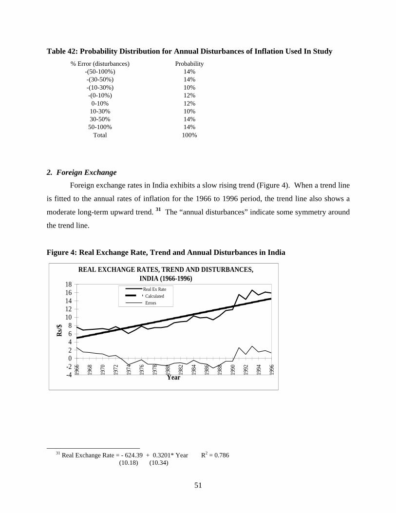
51
Table 42: Probability Distribution for Annual Disturbances of Inflation Used In Study
% Error (disturbances) Probability-(50-100%) 14%-(30-50%) 14%-(10-30%) 10%-(0-10%) 12%0-10% 12%
10-30% 10%30-50% 14%
50-100% 14%Total 100%
2. Foreign Exchange
Foreign exchange rates in India exhibits a slow rising trend (Figure 4). When a trend line
is fitted to the annual rates of inflation for the 1966 to 1996 period, the trend line also shows a
moderate long-term upward trend. 31 The “annual disturbances” indicate some symmetry around
the trend line.
Figure 4: Real Exchange Rate, Trend and Annual Disturbances in India
REAL EXCHANGE RATES, TREND AND DISTURBANCES, INDIA (1966-1996)
-4-202468
1012141618
1966
1968
1970
1972
1974
1976
1978
1980
1982
1984
1986
1988
1990
1992
1994
1996
Year
Rs/
$
Real Ex Rate
Calculated Errors
31 Real Exchange Rate = - 624.39 + 0.3201* Year R2 = 0.786 (10.18) (10.34)
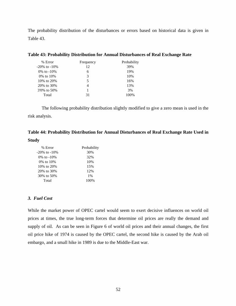
52
The probability distribution of the disturbances or errors based on historical data is given in
Table 43.
Table 43: Probability Distribution for Annual Disturbances of Real Exchange Rate
% Error Frequency Probability-20% to -10% 12 39%0% to -10% 6 19%0% to 10% 3 10%
10% to 20% 5 16%20% to 30% 4 13%3'0% to 50% 1 3%
Total 31 100%
The following probability distribution slightly modified to give a zero mean is used in the
risk analysis.
Table 44: Probability Distribution for Annual Disturbances of Real Exchange Rate Used in
Study
% Error Probability-20% to -10% 30%0% to -10% 32%0% to 10% 10%
10% to 20% 15%20% to 30% 12%30% to 50% 1%
Total 100%
3. Fuel Cost
While the market power of OPEC cartel would seem to exert decisive influences on world oil
prices at times, the true long-term forces that determine oil prices are really the demand and
supply of oil. As can be seen in Figure 6 of world oil prices and their annual changes, the first
oil price hike of 1974 is caused by the OPEC cartel, the second hike is caused by the Arab oil
embargo, and a small hike in 1989 is due to the Middle-East war.
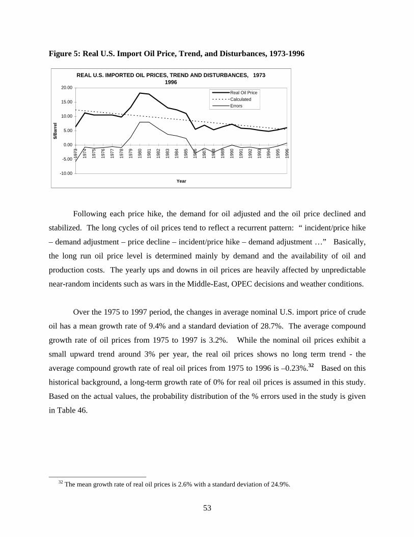
53
Figure 5: Real U.S. Import Oil Price, Trend, and Disturbances, 1973-1996
REAL U.S. IMPORTED OIL PRICES, TREND AND DISTURBANCES, 1973-1996
-10.00
-5.00
0.00
5.00
10.00
15.00
20.00
1973
1974
1975
1976
1977
1978
1979
1980
1981
1982
1983
1984
1985
1986
1987
1988
1989
1990
1991
1992
1993
1994
1995
1996
Year
$/B
arre
l
Real Oil Price
CalculatedErrors
Following each price hike, the demand for oil adjusted and the oil price declined and
stabilized. The long cycles of oil prices tend to reflect a recurrent pattern: “ incident/price hike
– demand adjustment – price decline – incident/price hike – demand adjustment …” Basically,
the long run oil price level is determined mainly by demand and the availability of oil and
production costs. The yearly ups and downs in oil prices are heavily affected by unpredictable
near-random incidents such as wars in the Middle-East, OPEC decisions and weather conditions.
Over the 1975 to 1997 period, the changes in average nominal U.S. import price of crude
oil has a mean growth rate of 9.4% and a standard deviation of 28.7%. The average compound
growth rate of oil prices from 1975 to 1997 is 3.2%. While the nominal oil prices exhibit a
small upward trend around 3% per year, the real oil prices shows no long term trend - the
average compound growth rate of real oil prices from 1975 to 1996 is –0.23%.32 Based on this
historical background, a long-term growth rate of 0% for real oil prices is assumed in this study.
Based on the actual values, the probability distribution of the % errors used in the study is given
in Table 46.
32 The mean growth rate of real oil prices is 2.6% with a standard deviation of 24.9%.

54
Table 45: Probability Distribution for Annual Disturbances of Real Oil Price
% Error Frequency Probability-40 to -30 1 4%-30 to -20 2 8%-20 to -10 6 25%-10 to 0 6 25%0 to-10 1 4%10 to 20 1 4%20 to-30 3 13%30 to 40 4 17%
Total 24 100%
Table 46: Probability Distribution for Annual Disturbances of Real Oil Price Used in Study
% Error Probability
-40% to -30% 4%-30% to -20% 13%-20% to -10% 25%-10% to 0%% 17%
0% to10% 8%10% to 20% 8%20% to-30% 13%30% to 40% 13%
Total 100%
4. Investment Cost Overrun
Construction cost overruns are more or less expected in large capital projects. The scale of cost
overruns varies from country to country, project to project and construction firm to construction
firm. A step distribution given in Table 40, Assumptions of Risk Variables, above is used to
represent the uncertainty of cost overruns.
5. Actual Plant Load Factor/Technical Risk
The actual energy delivered to the interconnection point depends on the plant’s design
and construction standards, and the IPP’s capability and willingness to maintain and repair the
plant and keep it in good running conditions. It also depends on the ability of the utility to take
delivery of the power.33 On the other hand, the expected demand for power or the demand
33 This is submitted to system and transmission constraints.
55
projection made by the utility may not be realized.34 This will also affect the actual plant load
factor. Actual Plant Load Factor may therefore affected by random factors. A normal distribution
which is given in Table 40 is therefore used.
6. Transfer Price
The transfer price of the power plant upon the consummation of the contract depends on
the conditions of the plant at the time, the valuation of the plant by an independent evaluator, and
the outcome of negotiation between the utility and the IPP. The final outcome is uncertain. A
normal distribution given in Table 40 is used to represent this uncertainty.
APPENDIX II NOTES ON POWER PURCHASE AGREEMENT
The power purchase agreement (the PPA) signed between the Sendara Pradesh State
Electricity Board (SPSEB) and Sendara Pradesh Power Partners Private Limited (SPPL) is based
on a fixed return on equity (fixed ROE). Accordingly, SPPL is guaranteed a 16% return on the
partners’ equity. Whether this 16% ROE is real or nominal is usually not specified in a PPA. It
is nevertheless a common practice to treat it as a nominal ROE. The real ROE will therefore
depend on the rate of inflation. For example, if a domestic inflation of 8% were expected, as in
our base case, then the underlying real ROE would be 7.41%. But if a domestic inflation of 3%
were considered, the underlying real ROE would be 12.62%.
The contract ROE is only used as part of the PPA payment formula to calculate the fixed
charge payment, it may or may not represent the true rate of return (ROR) to the IPP as the total
fixed charge payment also includes a horde of other variables and formula as will be explained
below. To determine the true ROR to the domestic and foreign equity owners we will have to
look at their separate cash flow.
34 This is the demand side quantity risk or demand risk.
56
The PPA payment formula consists basically of three parts: the fixed charge payment, the
variable charge payment and the incentive payment.
A. Fixed Charge Payment
The fixed charge payment is the main component of the PPA through which the IPP
recovers its capital investment costs as well as any other fixed charges. As noted in the
discussions in the main text and the sensitivity analysis of this study, the timing of various
payments (front-end-loading) can greatly affect the NPVs of the project. So is the possibility of
overcompensation - items such as depreciation payment, special appropriation and transfer price
can over compensate the investment cost, that is, the accumulated sum of these three items may
exceed the initial investment cost. In principle, since the fixed charge payment has already
included a payment on debt interest and a payment on the return on equity, the three items should
be strictly for the recapturing of the initial investment cost plus a proper return to the IPP
partners. This is an area that is quite often not clarified in most PPAs. Furthermore, the special
appropriation formula used in this study causes the depreciation plus special appropriation
payments to be highly front-end-loaded, resulting in 90%35 of the investment cost being
recaptured very early while the ROE payment continues through out the project life. Because of
the timing and structuring of the various items of the fixed charge payment, the actual rate of
return received by the IPP partners can only be determined through a proper cash flow analysis.
The different components of the fixed charge payment are:
Interest on Debt:
This is the interest portion of the loan repayments of the project.
Depreciation:
Depreciation payment is where the IPP are supposed to recover the investment costs or
the principal of their loans plus their equity investment. The exact computation is given by the
formula below.
35 This percentage depends on the Residual Value Ratio.
57
Depreciation Payment ={ (Investment Cost) * (1 - Residual Value Ratio) }/(Number of
Depreciation Periods)
The Depreciation Payment is subjected to a restriction explained in Special
Appropriation below.
Return on Equity:
Each year, the utility will pay the IPP a fixed percentage, 16% in our case, on the total
amount of the initial equity. For foreign equity, the return on equity is based on the 16% return
on the initial dollar value of the foreign equity, repaid in Rupees based on the most recent
exchange rate.
Interest on Working Capital:
The utility will pay the IPP for the interest on short-term loans taken out by the project to
finance the working capital necessary for the operating of the project. Working capital includes
fuel cost for one month, thirty days of fuel stock, one month of O & M expenses, and accounts
receivable equal two months of average billing.36
O & M and Insurance Expenses:
Operations and maintenance plus insurance expenses are assumed to be equal to 2.5% of
capital cost adjusted each year for inflation. The actual O&M plus insurance of SPPL may be
more or less than this presumed amount. In practice, this is an item that should be verified by the
utility. 37
Taxes on Income:
Corporate income taxes paid by SPPL are also covered by the utility. This is a feature to
ensure a net of tax ROE to the equity holders.38
Special Appropriation:
Special Appropriation is a payment made by the utility to the IPP whenever the
depreciation payment is less than the loan repayment subjected to the restriction that the
36 These items may change from case to case and may be negotiable. Two months of average billing is the
amount of receivable based on the quarterly billing period.37 In this study, the O&M plus insurance in the project cash flow is nevertheless assumed to be the same as the
amount specified in the contract.
58
accumulated sum of the special appropriation payments plus depreciation payments must not
exceed the investment cost less the residual value reservation. Once the accumulated sum
reaches the value equal to [(1-Residual Value Ratio)*Investment Cost], both the depreciation and
the special appropriation payments are reduced to zero.39
B. Variable Charge Payment
The variable charge payment compensates SPPL for the fuel cost, which is the main
variable input used in the generation of electricity. The variable charge payment formula is
simply a computational formula. While the formula itself may or may not be negotiable, it is
essential to be able to verify such values as heat rate of electricity and calorific value of fuel. The
following are the components of the variable charge payment computation formula:
Actual Energy (AEm):
Metered at the Interconnection Point, it does not include the auxiliary consumption used
to run the plant.
Fuel Cost (RFCm):
Fuel cost per kilogram in local currency, gross of tax, transportation, handling and
insurance costs.
Unit Heat Rate (UHRu):
Unit Heat Rate (UHRu) in kilocalories per kilowatt-hour for a unit u, is the number of
BTUs required to produce one kilowatt hour of electricity. In our base case, the UHR is assumed
to be 2,000 kilocalories per kilowatt-hour.
Gross Calorific Value of Fuel (GCVFu):
Gross Calorific Value of Fuel in kilocalories per kilogram. In our base case, the GCVF is
assumed to be 11,200 kilocalories per kilogram.
38 In this study, however, there is a five-year tax holiday, followed by five additional years with a corporate
income tax rate of 30% before the actual 46% rate comes into place.39 See main document for more details.

59
Auxiliary Consumption (AC):
The auxiliary power consumption by the plant is defined as a percentage of the total
amount of electricity generated.
Variable Charge Payment:
Variable Charge Payment = [(RFCm / GCVFu) * UHRu * AEm] / (1-AC)
C. Incentive Payment
This is a component of the PPA subject to negotiations. The incentive payment is based
on the “above average performance of the plant”. The various components of the incentive
payment formula are as follow:
Normative PLF:
The Normative PLF (NPLF) is the typical PLF for a given type of power plant according
to the operating conditions in that particular country and location. In our base case, the NPLF is
set at 68.49% which is specified by the Indian Government PPA directives.
Calculated PLF in billing period:
The calculated PLF in a billing period is defined as:
CPLF = (actual energy + deemed generation) / (installed capacity * number of hours in
the billing period).
Deemed Generation:
It is the amount of energy that the plant is capable of generating, which is not delivered to
the buyer for various reasons. It is defined as:
Deemed Generation = (declared availability * hours in period) – actual energy metered.
Declared Availability:
It is the generating capacity of the plant notified by the IPP to the buyer utility from time
to time. It is expressed in megawatts net of auxiliary consumption. Misdeclaration is subject to
penalty in order to discourage frauds. The penalty formula for misdeclaration may vary from

60
case to case. For example it may be defined as “For the misdeclared billing period, Declared
Availability shall be immediately reduced for the seven days after discovery, any payable
amount related to the Billing Period should be reduced or returned accordingly.” Or it may be
defined as “Hand back the recent availability payments, or alternatively, the IPP will in the
future receive incentive payments only for availability that has been demonstrated by actually
produced output.”
Incentive Points:
This is one of negotiable variables on the PPA payment. It is defined as a percentage (of
equity value). Our base case assumes that the incentive points is 0.7%.
Incentive Payment:
The incentive payment is calculated by the following formula:
Incentive Payment = Equity * (Calculated PLF – Normative PLF) * 0.7% * (days in
billing period/365)
D. Concluding Note
Because of the complexity of a PPA, it is impossible to know the true rate of return of the
project to the IPP partners without going through a thorough NPV cash flow analysis. The first
challenge to the evaluation of a PPA is therefore finding the true rate of return. The remaining
challenge is to determine a proper rate of return which corresponds to the risks of the project and
is acceptable to all parties of the BOT deal.


