
FACULTEIT WETENSCHAPPEN
Diagrammatic Monte Carlo study of
polaron systems
Jonas Vlietinck
Promotoren: Prof. Dr. Kris Van HouckeProf. Dr. Jan Ryckebusch
Proefschrift ingediend tot het behalen van de academische graad vanDoctor in de Wetenschappen: Fysica
Universiteit GentFaculteit WetenschappenVakgroep Fysica en SterrenkundeAcademiejaar 2014-2015

ii

Contents
Contents iii
1 Introduction 11.1 The Fermi gas as a model for strongly interacting Fermi systems . . . . . . . 11.2 The polaron: an impurity moving through a medium . . . . . . . . . . . . . . 31.3 Polarons in ultracold gases . . . . . . . . . . . . . . . . . . . . . . . . . . . . . 4
1.3.1 Two-body scattering at low energies . . . . . . . . . . . . . . . . . . . 41.3.2 The Fermi polaron Hamiltonian . . . . . . . . . . . . . . . . . . . . . . 61.3.3 The BEC polaron Hamiltonian . . . . . . . . . . . . . . . . . . . . . . 7
2 The Fermi polaron and its Green’s function 112.1 The Green’s function and the Feynman-Dyson perturbation series . . . . . . 112.2 Feynman diagrams for the Fermi polaron . . . . . . . . . . . . . . . . . . . . 132.3 Renormalization of the contact interaction . . . . . . . . . . . . . . . . . . . . 152.4 The one-body self-energy Σ(p,Ω) . . . . . . . . . . . . . . . . . . . . . . . . . 172.5 A variational calculation with 1 p-h excitations . . . . . . . . . . . . . . . . . 182.6 Constructing higher-order diagrams . . . . . . . . . . . . . . . . . . . . . . . . 202.7 Summing diagrams with diagrammatic Monte Carlo (DiagMC) . . . . . . . . 22
2.7.1 Updates of the DiagMC algorithm . . . . . . . . . . . . . . . . . . . . 252.7.2 Making a random walk in the configuration space of diagrams . . . . . 33
2.8 Quasiparticle properties of an impurity in a Fermi gas . . . . . . . . . . . . . 35
3 The 2D Fermi polaron 633.1 Renormalized interaction . . . . . . . . . . . . . . . . . . . . . . . . . . . . . 633.2 DiagMC for the 2D Fermi polaron . . . . . . . . . . . . . . . . . . . . . . . . 653.3 Diagrammatic Monte Carlo Study of the Fermi polaron in two dimensions . . 66
4 Large Bose polarons 814.1 Feynman diagrams for large polarons . . . . . . . . . . . . . . . . . . . . . . . 814.2 DiagMC for large polarons . . . . . . . . . . . . . . . . . . . . . . . . . . . . . 83
iii

iv Contents
4.3 DiagMC study of the acoustic and the BEC polaron . . . . . . . . . . . . . . 85
5 Summary 103
A Canonical transformation 107
B Fourier transform of Γ0(p,Ω) 111
C Samenvatting 115
Bibliography 119

CHAPTER 1
Introduction
1.1 The Fermi gas as a model for strongly interacting
Fermi systems
The simplest quantum many-body systems that one can imagine are the free Bose and
Fermi gas. Their thermodynamic quantities can easily be calculated within the framework
of statistical physics. If the particles of the many-body system are weakly interacting one
typically relies on perturbation theory to calculate the properties. In many realistic systems,
however, the interaction between the particles is far from weak and perturbation-theory
calculations mostly fail. This failure can be illustrated by considering the perturbation series
for the energy of an electron gas in a metal. Consider the following Hamiltonian:
H =
N∑
i=1
p2i
2m+
e2
4πε0
1
2
N∑
i,j=1(i 6=j)
1
‖ri − rj‖, (1.1)
with ε0 the vacuum permittivity, e the electron charge, m the electron mass, ri the position
operator and pi the momentum operator for the i-th electron. We neglect three-particle
interactions and assume that there are no external forces present. Upon calculating the
ground-state energy E0 of this system with the Coulomb interaction as a perturbation, we
get:
E0 = E(0)0 + E
(1)0 +∞+∞+ . . . . (1.2)
Calculating higher orders in perturbation theory gives divergences and perturbation theory
seems to fail in this case [1].
Some strongly interacting systems can be described by Landau Fermi liquid theory [2].
The theory constructs a model for the energies of the weakly excited states of the system.
1

2 1.1. The Fermi gas as a model for strongly interacting Fermi systems
Landau argued that numerous many-body systems of strongly interacting particles can be
mapped onto a system of weakly interacting elementary excitations above the ground state
[3](for example particle-hole excitations). Consider a Hamiltonian which is the sum of a
one-body operator T and a two-body interaction operator V . In standard second quantisation
notation, the Hamiltonian is written as (see, e.g., Ref. [4])
H = T + V
=∑
α,β
〈α|T |β〉c†αcβ +1
2
∑
αβρν
〈αβ|V |νρ〉c†αc†β cρcν .(1.3)
The operators c†α and cα denote the creation and annihilation of a fermion in the quantum
single-particle state |α〉 characterised by the quantum number(s) α. The Hamiltonian H in
Eq. (1.3) describes a system of strongly ’real’ interacting particles, that usually cannot be
solved by perturbation theory. In most many-body systems it turns out that a canonical
transformation (with canonical we mean that the commutation relations are preserved) can
be used to transform H into a Hamiltonian of the following form:
H = E0 +∑
γ
ε′γ a†γ aγ + f(. . . aγ . . . a
†γ . . .) , (1.4)
now written in terms of weakly interacting ’fictitious’ particles or elementary excitations
[1]. The operators a†γ and aγ denote the creation and annihilation for these elementary
excitations characterised by the quantum number γ above a ground-state energy E0. The term
f(. . . aγ . . . a†γ . . .) describes the interactions between elementary excitations and is assumed
to be small. The dispersion of the elementary excitations is given by ε′γ . These excitations
are the result of collective interactions in the system and give important information about
the macroscopic behavior of the system. The residual interaction term f(. . . aγ . . . a†γ . . .) will
give rise to a broadening ∆ε′γ of the energy levels ε′γ . By the uncertainty principle we know
that the elementary excitations will have a lifetime τγ ∼ ~(∆ε′γ)−1. In the Landau Fermi
liquid theory the decay rate of these excitations should be much less than their energy, or
∆ε′γ ε′γ . For f(. . . aγ . . . a†γ . . .)→ 0 the elementary excitations have a well-defined energy
and correspondingly an infinite lifetime. It should be noticed that the properties of these
elementary excitations can be totally different from those of the ’real’ particles.
We illustrate the ideas of Landau Fermi liquid theory with two examples. The first example
deals with electrons in a metal at a temperature T TF , with TF the Fermi temperature.
For a large class of metals the elementary excitations are particle-hole excitations. The
question arises whether the particle-hole excitations will be long-lived and have a narrow
width in energy. Landau realized that there is only a small phase space for scattering of
an electron just above the Fermi sea (FS) with an electron in the sea. This is a direct
consequence of the Pauli exclusion principle and leads to long-lived particle-hole excitations
if we consider scattering close to the Fermi surface. An electron above the Fermi sea can thus
be described as a free electron dressed with particle-hole excitations. These ideas show that
electrons in a metal often can be seen as freely moving particles. This free electron model
has also been verified experimentally in metals. The average distance between conduction

Chapter 1. Introduction 3
electrons in metals is about 2A. The mean free paths are however longer than 104 A at
room temperature and longer than 10 cm at 1K [5].
As a second example of a Landau Fermi liquid we consider an interacting Fermi gas at
T = 0 composed out of spin-up fermions and spin-down fermions. An attractive interaction
is considered, acting only between spin-up and spin-down fermions. The concentration of ↓atoms is assumed to be small, so that the ratio of densities x = n↓/n↑ 1, with n↓ (n↑) the
density of spin-down (spin-up) particles. A Fermi liquid model can be constructed and the
energy of the system becomes approximately [6, 7]:
E(x)
N↑=
3
5εF
(1−Ax+
m
m∗x5/3
), (1.5)
with εF the Fermi energy of the spin-up Fermi sea. The parameter A is related to the binding
energy of one spin-down atom to the Fermi gas of spin-up atoms and m∗ is the effective mass
of one spin-down impurity (quasiparticle). To find the parameters A and m∗ we need to
solve the problem of one spin-down fermion interacting with a spin-up sea. We will discuss
the Hamiltonian of this impurity system in more detail in Sec. 1.3.2.
1.2 The polaron: an impurity moving through a medium
In the last section we mentioned the problem of a single spin-down particle in a spin-up
Fermi sea. The problem of an impurity moving through a medium of identical particles has
been studied for decades. One of the first examples of the impurity system was studied by
Landau in 1933: an electron in an ionic lattice. Landau realized that an electron, by its
Coulomb interaction with the ions of the lattice, produces a polarization. The electron could
be seen as a rigid charge moving through the lattice carrying its polarization potential with
it, and hence Landau called it a polaron. In the case the lattice-deformation size (caused by
the electron) is larger than the lattice parameter, the lattice can be treated as a continuum.
In 1952, Frohlich derived a Hamiltonian Hpol for such a system [8]:
Hpol =∑
k
~2k2
2mc†kck
︸ ︷︷ ︸HIpol
+∑
q
~ω(q)b†qbq
︸ ︷︷ ︸HBpol
+∑
k,q
V (q)c†k+qck
(b†−q + bq
)
︸ ︷︷ ︸HIBpol
. (1.6)
Here, the c†k (ck) are the creation (annihilation) operators of the electron with mass m and
wave vector k. The kinetic energy of the electron is represented by the term HIpol and HB
pol
gives the energy of the phonons which carry the polarization. Thereby, the operator b†q (bq)
creates (annihilates) a phonon with wave vector q and energy ~ω(q). The term HIBpol denotes
the interaction between the charge carrier and the phonons with interaction strength V (q).
In the remainder of this work we take ~ = 1. A plethora of physical phenomena can be
described by the above Frohlich type of Hamiltonian by varying the dispersion ω(q) and
the interaction strength V (q), see for example [9]. Despite the importance of polarons in
semiconductor physics and in other branches of physics, studying polarons in solids has some

4 1.3. Polarons in ultracold gases
limitations. For example, the interaction strength will depend on the type of material and
exploring strongly interacting regimes can be difficult. The realization of a crystal at T = 0
poses also difficulties and the transformation of such a crystal to a gas of non-interacting
phonons is also an idealization of reality. One could include an interaction term for the
phonons, yet the price we pay is a more complicated model that is difficult to solve. In the
next section, a more controllable and clean medium will be presented which will allow us to
make a better mapping for this experimental system on a theoretical polaron model.
1.3 Polarons in ultracold gases
Since the first experimental realization of Bose Einstein condensation (BEC) in 1995 [10–12],
ultracold gases have become very important in the study of quantum many-body physics.
Within the last decade, fundamental phenomena like coherence, superfluidity, quantum phase
transitions, . . . were studied in these systems. It was soon realized that ultracold gases offer
a unique test system that could be used as a quantum simulator of strongly interacting
many-body physics [13]. For example, an impurity immersed in a BEC (the BEC polaron)
can be represented, under certain conditions ( see Sec. 1.3.3), by a Hamiltonian which has
the same structure as Hpol.
In ultracold gases we have the ability to tune the s-wave scattering length to arbitrary
values by means of Feshbach resonances [14], which offers the possibility to study weakly and
strongly interacting systems. Consider for example the case of a two-component Fermi gas
(with spin-down and spin-up fermions). If we start from a weakly interacting Fermi gas and
increase the attraction between the fermions we will end up with a gas of bosonic molecules
that form a BEC at sufficiently low temperature. What happens is the so-called BEC-BCS
crossover [15], which smoothly converts a gas of fermions into a gas of bosons. The extremely
imbalanced case with one spin-down fermion and N spin-up fermions is called the Fermi
polaron [16].
Before we start discussing polaron systems in ultracold gases, we will first take a brief
look at two-body scattering at low energy in Sec. 1.3.1. In Sec. 1.3.2 the Fermi polaron
Hamiltonian in three dimensions (3D) will be introduced and in Sec. 1.3.3 we will set up a
Hamiltonian for the 3D BEC polaron.
1.3.1 Two-body scattering at low energies
Since we are dealing with dilute gases, the following relation between the interaction range
R of the potential and the density ρ is valid:
Rρ1/3 1 . (1.7)
This means that the average distance between two particles is much larger than the range of
the interaction, which allows us to restrict ourselves to binary scattering.
We consider an ultracold collision that involves two distinguishable particles in the
center-of-mass (c.m.) frame. The relative wave function in 3D at a distance r far beyond the

Chapter 1. Introduction 5
interatomic potential is given by:
ψ = eikz + f(k, θ)eikr
r, (1.8)
where eikz represents the incoming plane wave with wave vector k along the z-axis. We
assume the interaction between the atoms to be spherically symmetric. The scattering
amplitude can be written as an expansion in partial waves:
f(k, θ) =
∞∑
l=0
fl(k, θ) =1
2ik
∞∑
l=0
(2l + 1)(ei2δl − 1)Pl(cos θ) , (1.9)
with δl the phase shift of the scattered wave and Pl(cos θ) the Legendre polynomials. Since
we are interested in scattering at low momenta, s-wave (l = 0) scattering will be dominant
over all other partial waves. So, the scattering amplitude becomes [17]:
f(k, θ) ≈ f0(k, θ) =1
2ik(e2iδs − 1) =
1
k cot δs − ik. (1.10)
In this expression k cot δs can be further expanded:
k cot δs ≈ −1
as+reff
2k2 + . . . , (1.11)
where as is the s-wave scattering length and reff the effective range of the interaction potential.
The “. . .” represent higher order terms in k2. Since we consider low-energy scattering in a
dilute gas, we can write that R λ, with λ the de Broglie wavelength. This means that the
fine details of the potential are not required and any potential that reproduces the desired
set of scattering parameters (a, reff, . . .) is a good one. This ’fictitious’ potential is also called
an effective potential. Of course we want to choose a potential that makes our calculations
as simple as possible. An obvious candidate is given by V (r) = g0δ(r), with g0 the coupling
constant. We regularise the Dirac-delta interaction potential by putting the particles on a
lattice. The following relation between g0 and as can be obtained [18]:
1
g0=
m
4πas− 1
(2π)3
∫
Bdqm
q2, (1.12)
where the integral is over the first Brillouin zone B =]− π/b, π/b]3 of the reciprocal lattice,
with b the lattice spacing. In Sec. 2.3 the continuum limit will be taken (b→ 0 and g0 → 0−).
In two dimensions (2D) we wish to write a relation between the bare coupling constant
g0 and the two-body binding energy εB in vacuum. Such a bound state always exists in two
dimensions, as long as the interaction potential is attractive. The relation between εB and
g0 can be established by considering the bound state |ψp〉 :
|ψp〉 =∑
q
φq|p− q,q〉 , (1.13)
with p−q and q the momenta of the non-identical particles and φq the Fourier representation
of the wave function for the relative motion of the two bound particles. Let us denote the

6 1.3. Polarons in ultracold gases
two particles by spin-↑ and spin-↓. The Hamiltonian reads:
H =∑
q∈B,σ=↑↓εqσ c
†qσ cqσ +
g0
V∑
p,q,q′∈Bc†p−q↑c
†q′+q↓cq′↓cp↑ , (1.14)
with the dispersion εqσ = q2
2mσand mσ the mass of the spin-σ fermion, and V the area of
the system. (In Sec. 3.1 the thermodynamic limit, V → ∞ will be taken). Wave vectors are
summed over the first Brillouin zone B =]− π/b, π/b]2 in two dimensions. The operators c†qσ(cqσ) create (annihilate) particles with momentum q and spin σ. The energy of the state
|ψp〉 is given by
〈ψp|H|ψp〉 =∑
q∈B|φq|2(εq↓ + εp−q↑) +
g0
V∑
q,q′∈Bφqφ
∗q′ , (1.15)
To minimize 〈ψp|H|ψp〉 with the constraint 〈ψp|ψp〉 = 1 we consider the function Λ:
Λ = 〈ψp|H|ψp〉 − εB
∑
q∈B|φq|2 − 1
, (1.16)
where εB can also be interpreted as the Lagrange multiplier associated to the normalization
of |ψp〉. The minimization of Λ with respect to φq gives:
∂Λ
∂φq= 0 ,
(εq↓ + εp−q↑)φq +g0
V∑
q′∈Bφq′ = εBφq ,
(1.17)
φq = −g0
V
∑q′∈B
φq′
εp−q↑ + εq↓ − εB. (1.18)
From Eq. (1.18) if follows that for large |q| the following relation holds
φq ∝1
q2. (1.19)
By applying the summation∑
q on both sides of Eq. (1.18) and taking the c.m. momentum
p = 0, we get a relation between g0 and εB :
−1
g0=
1
V∑
q∈B
1
εq↑ + εq↓ − εB. (1.20)
1.3.2 The Fermi polaron Hamiltonian
Before we set up a Hamiltonian for the Fermi polaron we first take at look at the interac-
tions among the spin-up fermions and the interaction between the spin-down fermion (the
impurity) and the spin-up sea. The scattering of two indentical spin-up fermions in the
c.m. frame at distances larger than the range of the interatomic potential is determined

Chapter 1. Introduction 7
by the antisymmetrized form of the wave function of Eq. (1.8). The interchange of two
particle coordinates corresponds to changing the sign of the relative coordinate r → −r,or, in spherical coordinates, r → r, φ → φ + π, θ → π − θ and the antisymmetrized wave
function is [19]:
ψ = eikz − e−ikz + [f(θ)− f(π − θ)] eikr
r. (1.21)
The differential cross section is given by
dσ
dΩ= |f(θ)− f(π − θ)|2 , (1.22)
with σ the cross section and Ω the solid angle. For s-wave scattering there is no θ dependence
in f(θ) (see Eq. (1.10)) and consequently the cross section vanishes for fermions in the same
state. As shown in Ref. [20] p-wave scattering is strongly suppressed if we consider low-energy
scattering and therefore scattering between identical fermions will be neglected. The matrix
element of the interaction between the impurity and a spin-up fermion in position space is
denoted by V↓↑(r− r′).The Hamiltonian HFP of the Fermi polaron is
HFP = H0 + H↓↑ , (1.23)
with
H0 =∑
k,σ=↑↓εkσ c
†kσ ckσ , (1.24)
H↓↑ =1
V∑
k,k′,q
V↓↑(q)c†k+q↑c†k′−q↓ck′↓ck↑ . (1.25)
The operators c†kσ (ckσ) create (annihilate) fermions with momentum k and spin σ. The
volume is denoted by V. The spin-σ fermions have mass mσ and dispersion εkσ = k2/2mσ.
For the interaction between the spin-down impurity and a spin-up fermion we adopt a Dirac
delta potential, V↓↑(r− r′) = g0δ(r− r′) with g0 the coupling constant, and in momentum
space V↓↑(k) = g0. To regularise the ultraviolet divergences that appear because of this
choice, we will put the fermions again on the lattice, which naturally truncates the momentum
integration.
1.3.3 The BEC polaron Hamiltonian
The following Hamiltonian can be used to describe an impurity in a bath of interacting
bosonic particles:
H =∑
p
p2
2mIc†pcp +
∑
k
εka†kak +
1
2V∑
k,k′,q
VBB(q)a†k′−qa†k+qakak′
+1
V∑
k,k′,q
VIB(q)c†k+qcka†k′−qak′ ,
(1.26)
8 1.3. Polarons in ultracold gases
with the dispersion given by εk = k2/2mB , and V the volume of the system. The operators
a†k(ak) create (annihilate) bosons with momentum k and mass mB. The operators c†p(cp)
create (annihilate) the impurity with momentum p and mass mI . The interaction potential
in momentum space between bosons of the bath is given by VBB(q), and VIB(q) represents
the interaction potential of the impurity with a boson of the bath. At sufficiently low
temperatures the bosons will form a Bose-Einstein condensate. If N − N0 N0 is valid,
with N0 the number of bosons in the condensate and N = 〈N〉 the average total particle
number, the Bogoliubov approximation can be applied [4, 21]:
a†0 ≈ a0 ≈√N0 , (1.27)
and the operators can be treated as real numbers. As a consequence the Hamiltonian H will
no longer conserve particle number. The number operator N is given by:
N = N0 +∑
|k|6=0
a†kak . (1.28)
By applying the Bogoliubov approximation on Eq. (1.26), we get :
H ≈∑
p
p2
2mIc†pcp +
N0
V VIB(0) +1
2VN20VBB(0) +
∑
|k|6=0
εka†kak
+N0
2V∑
|k|6=0
VBB(k)(a†ka†−k + aka−k) + 2
N0
V∑
|k|6=0
VBB(k)a†kak
+
√N0
V∑
|k|6=0,p
VIB(k)c†p+kcp(a†−k + ak)
:=HBP .
(1.29)
We ignore terms with more than three non-condensate operators, which is a good approxi-
mation if N −N0 N0.
We replace the actual interaction potentials with pseudo-potentials, VIB(k) = gIB and
VBB(k) = gBB. The momentum independent matrix elements gIB and gBB can again be
chosen such that the two-body scattering properties in vacuum are correctly reproduced.
Like in Sec. 1.3.1, we have a relation between gBB and the boson-boson scattering length
aBB (and a similar relation for gIB and the impurity-boson scattering length aIB):
4πaBBmB
= gBB −mBg2BB
∫dq
(2π)3
1
q2+ . . . . (1.30)
We keep only the first-order Born result:
gBB =4πaBBmB
. (1.31)
Similarly, we have
gIB =2πaIBmr
, (1.32)

Chapter 1. Introduction 9
with the reduced mass mr = mImBmI+mB
. The second order contribution in Eq. (1.30) diverges
for high momenta. This divergence stems from our particular choice with regard to the
momentum dependence of the pseudo-potential. To regularise this ultraviolet divergence we
introduce a global momentum cut-off in the sums (or integrals) over momenta. We will see in
Sec. 4.3 that the divergence of the second order Born term cancels with another divergence
which appears in the ground-state energy of the interacting Bose gas.
A canonical transformation can be applied to Eq. (1.29) (see appendix A for the derivation),
which leads to a Frohlich type of Hamiltonian:
HBP =E0 + n0gIB +∑
p
p2
2mIc†pcp +
∑
|k|6=0
ω(k)b†kbk
+∑
|k|6=0,p
VBP (k) c†p+kcp(b†−k + bk
).
(1.33)
The creation (annihilation) operator b†k (bk) represent now the creation (annihilation) of a
Bogoliubov excitation. The quasiparticle vacuum energy is
E0 =V2n2gBB +
1
2
∑
k
(ω(k)− εk − n0gBB) , (1.34)
with the dispersion relation ω(k) given by
ω(k) = ck
√1 +
(ξk)2
2, (1.35)
the healing length of the condensate ξ = 1√8πn0aBB
, the speed of sound in the condensate
c =√
4πn0aBBmB
and the density of the condensed bosons n0 = N0/V and the average total
density n = 〈N〉/V . The interaction matrix element VBP (k) between a Bogoliubov excitation
and the impurity is given by
VBP (k) =
√N0gIBV
((ξk)2
(ξk)2 + 2
)1/4
. (1.36)

10 1.3. Polarons in ultracold gases

CHAPTER 2
The Fermi polaron and its Green’s function
To calculate the properties of the Fermi polaron, we will use the Green’s function formalism
(see for example [3, 4, 21]). From the knowledge of the Green’s function all relevant properties
can be extracted. We will calculate the Green’s function of the Fermi polaron by means
of a Feynman-Dyson series expansion. The terms in this series can be identified with
Feynman diagrams. We will argue that the diagrammatic Monte Carlo (DiagMC) method, an
importance sampling Monte Carlo (MC) method, is a very powerful method to sample over
a large number of diagrams. This technique will allow us to evaluate the Green’s function to
a high precision.
2.1 The Green’s function and the Feynman-Dyson per-
turbation series
The polaron’s quasiparticle properties can be extracted from the impurity’s Green’s function
defined as
G↓(p, τ) = −θ(τ)〈ΦN↑0 |cp↓(τ)c†p↓(0) |ΦN↑0 〉 , (2.1)
with cp↓(τ) the annihilation operator of the ‘spin-↓’ impurity in the Heisenberg picture,
cp↓(τ) = e(HFP−µN↓−µ↑N↑)τ cp↓e−(HFP−µN↓−µ↑N↑)τ , (2.2)
and θ the Heaviside function. The propagator G↓(p, τ) is written in the momentum imaginary-
time representation, µ is a free parameter, Nσ is the number operator for spin-σ particles,
and µ↑ is the chemical potential of the spin-up sea. The state
|ΦN↑0 〉 = |〉↓|FS(N↑)〉 , (2.3)
11

12 2.1. The Green’s function and the Feynman-Dyson perturbation series
consists of the spin-down vacuum and the non-interacting spin-up Fermi sea. Since we
are dealing with an impurity spin-down atom, G↓ is only non-zero for times τ > 0. The
ground-state energy and Z-factor can be extracted from the Green’s function of Eq. (2.1).
Inserting a complete set of eigenstates |ΨN↑n 〉 of the full Hamiltonian HFP for one spin-down
particle and N↑ spin-up particles into Eq. (2.1) gives
G↓(p, τ) = −θ(τ)∑
n
|〈ΨN↑n |c†p↓|Φ
N↑0 〉|2e−(En(N↑)−EFS−µ)τ
τ→+∞= − Zpol(p) e−(Epol(p)−µ)τ ,
(2.4)
with Epol(p) the energy of the polaron at momentum p for the impurity and En(N↑) the
energy eigenvalues of the Hamiltonian HFP of Eq. (1.23). The energy of the ideal spin-up
Fermi gas is EFS = 3 εFN↑/5, with εF = k2F /(2m↑) the Fermi energy and kF the Fermi
momentum. This asymptotic behavior implies a pole singularity for the Green’s function in
imaginary-frequency representation
G↓(p, ω) =
∫ +∞
0
dτ eiωτG↓(p, τ)
=Zpol(p)
iω + µ− Epol(p)+ regular part .
(2.5)
The Feynman-Dyson perturbation series for the one-particle Green’s function in imaginary
time τ and momentum p is given by
G↓(p, τ) =−∞∑
n=0
(−1)n1
n!
∫ ∞
0
dτ1 . . .
∫ ∞
0
dτn
〈ΦN↑0 |T[H↓↑I(τ1) . . . H↓↑I(τi+1) . . . H↓↑I(τn)cp↓I(τ)c†p↓I(0)
]|ΦN↑0 〉connected ,
(2.6)
with T the time-ordered product and the operators with subscript I are given in the interaction
picture. Each term in this series can be visualized by Feynman diagrams, whereby only the
connected diagrams have to be taken into account. The operator cpσI(τ) in the interaction
picture is defined as:
cpσI(τ) ≡ eK0τ cpσe−K0τ , (2.7)
with
K0 =∑
kσ
(εkσ − µσ)c†kσ ckσ ≡ H0 −∑
σ
µσNσ , (2.8)
where we introduce the notation µ↓ = µ for convenience. The time dependence of the creation
(annihilation) operators c†pσI(τ) (cpσI(τ)) in the interaction picture is the solution of the
differential equation [4]:
−∂cpσI(τ)
∂τ=[cpσI(τ), K0
]
= eK0τ (εpσ − µσ)[cpσ, c
†pσ cpσ
]e−K0τ
= (εpσ − µσ)cpσI(τ) .
(2.9)

Chapter 2. The Fermi polaron and its Green’s function 13
Thus,
cpσI(τ) = cpσe−(εpσ−µσ)τ , (2.10)
c†pσI(τ) = c†pσe(εpσ−µσ)τ . (2.11)
For an operator OS in the Schrodinger picture the time-dependence of the operator OI(τ) in
the interaction picture is given by
OI(τ) = eK0τ OSe−K0τ . (2.12)
2.2 Feynman diagrams for the Fermi polaron
To calculate G↓(p, τ) with the use of Eq. (2.6) we need to evaluate the matrix elements in
this expression. In this section we will calculate some low order contributions (n = 1 and
n = 2). In the end of this section, we will show how to create higher order diagrams for the
Fermi polaron. First we give the expressions of the free Green’s function. The free Green’s
function for the impurity with momentum p is given by
G0↓(p, τ) = −θ(τ)〈ΦN↑0 |T
[cp↓I(τ)c†p↓I(0)
]|ΦN↑0 〉 = −θ(τ)e−(εp↓−µ)τ , (2.13)
with εp↓ = p2
2m↓the impurity dispersion. From now on, we drop the subscript I, since in
the following all time-dependent operators will be in the interaction picture, unless stated
otherwise. The free Green’s function for the spin-up particles in the Fermi sea with momentum
k is given by
G0↑(k, τ) = −〈ΦN↑0 |T
[ck↑(τ)c†k↑(0)
]|ΦN↑0 〉
= −θ(k − kF )e−(εk↑−εF )τθ(τ) + θ(kF − k)e−(εk↑−εF )τθ(−τ) ,(2.14)
with the dispersion given by εk↑ = k2
2m↑. The contribution D1 in Eq. (2.6) for n = 1 is
D1 =
∫ ∞
0
dτ1〈ΦN↑0 |T[H↓↑(τ1)cp↓(τ)c†p↓(0)
]|ΦN↑0 〉
=g0
(2π)3
∫ ∞
0
dτ1
∫
B,|qh|<kFdqh〈ΦN↑0 |T
[c†p↓(τ1)cp↓(τ1)c†qh↑(τ1)cqh↑(τ1)cp↓(τ)c†p↓(0)
]|ΦN↑0 〉
=g0
(2π)3
∫ τ
0
dτ1
∫
B,|qh|<kFdqh
∑
n,n′
〈ΦN↑0 |cp↓(τ)c†p↓(τ1)|ΦN↑n 〉〈ΦN↑n |c†qh↑(τ1)cqh↑(τ1)|ΦN↑n′ 〉
〈ΦN↑n′ |cp↓(τ1)c†p↓(0)|ΦN↑0 〉
= g0
∫ τ
0
dτ1G0↓(p, τ − τ1)G0
↓(p, τ1) n↑ ,
(2.15)
with |ΦN↑n 〉 a complete set of eigenstates of the Hamiltonian H0. Note that we have taken
the thermodynamic limit, and n↑ is the density of spin-↑ fermions. The contribution D2 for

14 2.2. Feynman diagrams for the Fermi polaron
p p p p p
0τ1τ2τ0τ1τ 0τ1τ2τ
pp
q1 q2
q1q1 q2
p+ q1 − q2
Figure 2.1 – First and second order diagrams. Imaginary times run from right to left. The straight
line represents the propagation of the impurity. The forward oriented arc represents a particle of the
Fermi sea, a backward propagating arc a hole in the Fermi sea. The interaction vertices are denoted
by dots.
n = 2 in Eq. (2.6) is
D2 = −∫ ∞
0
dτ2
∫ τ2
0
dτ1〈ΦN↑0 |T[H↓↑(τ1)H↓↑(τ2)cp↓(τ)c†p↓(0)
]|ΦN↑0 〉
=−g2
0
(2π)6
∫ τ
0
dτ2
∫ τ2
0
dτ1
(∫
B,|q1|<kF ,|q2|>kFdq1dq2 c†p+q1−q2↓(τ1)Êcp↓(τ1)Î
× c†q2↑(τ1)Ìcq1↑(τ1)Íc†p↓(τ2)Ëcp+q1−q2↓(τ2)Êc†q1↑(τ2)Ícq2↑(τ2)Ìcp↓(τ)Ëc†p↓(0)Î
+
∫
B,|q1|<kF ,|q2|<kFdq1dq2 c†p↓(τ1)Êcp↓(τ1)Îc†q1↑(τ1)
Ìcq1↑(τ1)Ìc†p↓(τ2)Ë
× cp↓(τ2) Ê c†q2↑(τ2)Ícq2↑(τ2)Ícp↓(τ)Ëc†p↓(0)Î).
(2.16)
We use Wick’s theorem in the last line, with the contraction between a creation and an
annihilation operator given by:
c†pσ(τ1)Êcp′σ′(τ2)Ê = T(c†pσ(τ1)cp′σ′(τ2)
)−N
(c†pσ(τ1)cp′σ′(τ2)
)
= G0σ(p, τ2 − τ1)δσ,σ′δ(p− p′) .
(2.17)
with T (. . .) the time ordered product and N(. . .) the normal ordered product. The contribu-
tion D2 can now be written in terms of Green’s functions:
D2 =−g2
0
(2π)6
∫ τ
0
dτ2
∫ τ2
0
dτ1
( ∫
B,|q1|<kF ,|q2|>kFdq1dq2 G0
↓(p + q1 − q2, τ2 − τ1)
×G0↓(p, τ1)G0
↑(q2, τ2 − τ1)G0↑(q1, τ1 − τ2)G0
↓(p, τ − τ2)
−∫
B,|q1|<kF ,|q2|<kFdq1dq2 G0
↓(p, τ2 − τ1)G0↓(p, τ − τ2)G0
↓(p, τ1)
× G0↑(q1, 0
−) G0↑(q2, 0
−)
).
(2.18)

Chapter 2. The Fermi polaron and its Green’s function 15
Γ0
Figure 2.2 – Graphical representation of ladder diagrams. Imaginary times runs from right to left.
From the previous examples we can already deduce some characteristics of the diagrams.
Since we only have one spin-down particle, there is only one possibility for the contractions
of the operators of the spin-down particle. To construct a diagram, the propagation in
(imaginary) time of the impurity can be depicted with a straight line, which we will call the
backbone line (BBL) of the diagram. Another property that can be seen from the examples
is that no time can become larger than τ . So, the upper limits +∞ in Eq. (2.6) can be
replaced by τ . A third property is that only the impurity can create particles and holes in
the Fermi sea, and as a consequence we have no disonnected diagrams.
In Fig. 2.1 we show the diagrams which correspond to the first and second order con-
tributions. Creating higher order diagrams can be done easily in the following way. First,
draw a BBL which goes from 0 to τ . Then, add vertices on the BBL that represent the
bare interaction matrix element g0, and the number of vertices equals the order n. Next,
draw particles and hole lines onto the BBL in a way that each vertex has two incoming lines
and two outgoing lines. Since the impurity is propagating forward and the particle number
should be conserved at each time, the number of the particles and holes in the Fermi sea
should always be equal at each time. Each diagram acquires a sign (−1)n+L, with n the
order and L the number of loops. Each hole line acquires a momentum |q| < kF , a particle
line will have a momentum |q| > kF . The momentum of the impurity is then fixed by the
conservation of momentum at each vertex.
2.3 Renormalization of the contact interaction
As explained in Sec. 1.3.1, we have the freedom to choose any effective potential V↓↑(k) as
long as it reproduces the desired scattering length as. Because we have set V↓↑(k) = g0,
however, ultraviolet divergences arise. Those were regularised by considering fermions that
move on a lattice. The continuum limit cannot be taken directly. For example: Eq. (2.18) will
diverge if the lattice spacing l→ 0 (and keeping g0 fixed). To overcome this problem we will
show in this section that the continuum limit can be taken after a suitable renormalization
of the bare contact interaction. To this end we evaluate an infinite series of so-called ladder
diagrams (see Fig. 2.2) Γ0(p, τ) given by:
Γ0(p, τ) = g0 − g0
∫ τ
0
dτ11
(2π)3
∫
B,|q|>kF
dq G0↓(p− q, τ1)G0
↑(q, τ1)Γ0(p, τ − τ1) . (2.19)
Beside the time, Γ0(p, τ) only depends on the total incoming momentum p. This is a
consequence of the fact that the interaction potential V↓↑(k) is a Dirac delta-function, so
that V↓↑(k) does not depend on the momentum transfer. This can be written in imaginary

16 2.3. Renormalization of the contact interaction
frequency domain,
1
Γ0(p,Ω)=
1
g0+
1
(2π)4
∫ +∞
−∞dω
∫
B,|q|>kF
dq G0↓(p− q,Ω− ω)G0
↑(q, ω) , (2.20)
with Ω and ω imaginary frequencies. The free propagators G0↓(p− q,Ω− ω) and G0
↑(q, ω) in
imaginary frequency domain are given by
G0↓(p− q,Ω− ω) = 1
i(Ω−ω)− (p−q)2
2m↓+µ
;
G0↑(q, ω) = 1
iω− q2
2m↑+εF
.(2.21)
By making use of the residue theorem the integral over frequencies can be calculated.
Identifying the poles ω1 and ω2 givesω1 = Ω + i
((p−q)2
2m↓− µ
);
ω2 = −i( q2
2m↑− εF ) .
(2.22)
By closing the contour in the lower half of the complex plane, and choosing µ < 0, one gets:
1
Γ0(p,Ω)=
1
g0− 1
(2π)3
∫
B,|q|>kFdq
1
iΩ− (p−q)2
2m↓+ µ− q2
2m↑+ εF
. (2.23)
With the use of Eq. (1.12) the interaction strength parameter g0 can be removed in favour of
the scattering length as in Eq. (2.23),
1
Γ0(p,Ω)=
mr
2πas− 1
(2π)3
∫
B,|q|>kFdq
1
iΩ− (p−q)2
2m↓+ µ− q2
2m↑+ εF
− 1
(2π)3
∫
Bdq
2mr
q2.
(2.24)
By grouping the two integrands together, this expression is well-defined in the zero-range
limit. We can take the continuum limit l→ 0 and g0 → 0− such that as is fixed. To evaluate
Eq. (2.24) we write Γ0−1(p,Ω) as
Γ0−1(p,Ω) = Γ0−1
(p,Ω)− Π(p,Ω) , (2.25)
with
1
Γ0(p,Ω)=
mr
2πas−∫
dq
(2π)3
1
iΩ− (p−q)2
2m↓+ µ− q2
2m↑+ εF
+2mr
q2
, (2.26)
and Π(p,Ω):
Π(p,Ω) = −∫
dq
(2π)3
θ(kF − |q|)iΩ− q2
2m↑− (p−q)2
2m↓+ µ+ εF
. (2.27)
The function Γ0−1
(p,Ω) can be calculated analytically, for Ω 6= 0 or µ < −εF :
1
Γ0(p,Ω)=
mr
2πas− 1√
2πm3/2r
√−iΩ− µ+
p2
2(m↑ +m↓)− εF , (2.28)

Chapter 2. The Fermi polaron and its Green’s function 17
with mr =m↑m↓m↑+m↓
. To construct Feynman diagrams (see Sec. 2.6) we will use Γ0(p, τ)
in the momentum-imaginary-time representation as a renormalized interaction or dressed
interaction. We get Γ0(p, τ) by calculating the following Fourier transform:
Γ0(p, τ) =1
2π
∫ +∞
−∞dΩ Γ0(p,Ω)e−iτΩ . (2.29)
We obtain for Γ0(p, τ), if µ < −εF − 12mra2
s(see appendix B):
Γ0(p, τ) = − 4π
(2mr)3/2e
(µ+εF− p2
2(m↓+m↑))τ(
1√πτ
+1
as√
2mre
τ2mra2
s erfc
(−√
τ
2mr
1
as
)),
(2.30)
with erfc the complementary error function. Consider now the function (Γ0 − Γ0)(p, τ):
Γ0(p, τ)− Γ0(p, τ) =1
2π
∫ +∞
−∞dΩ(
Γ0(p,Ω)− Γ0(p,Ω))e−iτΩ . (2.31)
The function(
Γ0(p, τ)− Γ0(p, τ))
can be computed numerically and is a well-behaved
and bounded function, and therefore it can be tabulated very accurately in a (|p|, τ) grid.
Whenever Γ0(p, τ) is needed, we calculate it as a sum of the analytically obtained function
Γ0(p, τ) and the tabulated function(
Γ0(p, τ)− Γ0(p, τ))
.
2.4 The one-body self-energy Σ(p,Ω)
In this section we introduce the one-body self-energy Σ(p,Ω), with p the momentum of the
impurity and Ω the imaginary frequency, and show its relation with the polaron ground-state
energy Epol(p) and the Z-factor Zpol(p). The one-body self-energy Σ(p,Ω) is related to the
Green’s function G↓(p,Ω) by means of the Dyson equation:
G↓(p,Ω) = G0↓(p,Ω) +G0
↓(p,Ω)Σ(p,Ω)G↓(p,Ω) . (2.32)
To emphasise the dependence of G↓(p, τ) and Σ(p, τ) on the free parameter µ, we use the
notation:
G↓(p, τ) ≡ G↓(p, τ, µ) = G↓(p, τ, 0) eµτ ,
Σ(p, τ) ≡ Σ(p, τ, µ) = Σ(p, τ, 0) eµτ . (2.33)
The simple exponential dependence on µ follows from the fact that there is a backbone line.
To obtain a relation between the one-body self-energy and Epol(p) [22], consider the poles
for G↓(p, τ) given in Eqs. (2.32) and (2.5):
iΩ + µ− Epol(p)
Zpol(p)= G0
↓−1
(p,Ω, µ)− Σ(p,Ω, µ)
= iΩ− p2
2m↓+ µ− Σ(p,Ω, µ) .
(2.34)

18 2.5. A variational calculation with 1 p-h excitations
For small values of Ω we can use the following Taylor expansion:
Σ(p,Ω, µ) = Σ(p,Ω = 0, µ) + Ω∂Σ(p,Ω, µ)
∂Ω
∣∣∣∣Ω=0
+ . . . . (2.35)
By differentiating Eq. (2.33) with respect to µ and integrating over τ we obtain that∂Σ(p,Ω,µ)
∂Ω
∣∣∣Ω=0
= i ∂Σ(p,Ω=0,µ)∂µ . Since µ is a free parameter it is allowed to set it equal to
Epol(p). With the aid of Eq. (2.35), we can rewrite Eq. (2.34) for small values of Ω as
iΩ
Zpol(p)= iΩ− p2
2m↓+Epol(p)−Σ(p,Ω = 0, µ = Epol(p))− iΩ ∂Σ(p,Ω = 0, µ)
∂µ
∣∣∣∣µ=Epol(p)
.
(2.36)
Identifying the real and imaginary parts in Eq. (2.36) gives the following relations for Epol(p)
and Zpol(p):
Epol(p) =p2
2m↓+ Σ (p,Ω = 0, µ = Epol(p)) , (2.37)
Zpol(p) =1
1− ∂Σ(p,Ω=0,µ)∂µ
∣∣∣µ=Epol(p)
. (2.38)
In the previous section we have summed an infinite subclass of diagrams, which resulted
in a renormalized or dressed interaction Γ0. We are now able to draw Feynman diagrams that
are well-defined in the continuum limit. Let us evaluate the one-body self-energy Σ(1)(p,Ω)
built from one renormalized interaction Γ0 and one spin-↑ hole propagator G0↑, as shown in
Fig. 2.3. In the next section we will see that Σ(1)(p,Ω) includes all the 1 p-h excitations
of the polaron system. By making use of the Feynman rules (see for example [4, 21]) the
self-energy Σ(1)(p,Ω) is given by:
Σ(1)(p,Ω) =
∫
|q|<kF
dq
(2π)3
∫dω
2πΓ0(p + q,Ω + ω)G0
↑(q, ω) , (2.39)
with ω the imaginary frequency and q the momentum of the spin-up propagator. In Sec. 2.6
the diagram of Fig. 2.3 will be called the first order diagram.
2.5 A variational calculation with 1 p-h excitations
In this section we calculate the ground-state energy of the Fermi polaron by using a variational
method with a related wave function that includes 1p-h excitations [23].
One proposes a state |ψ〉
|ψ〉 = φ0|0, FS〉+∑
k,q∈Bφk,q|k,q〉 . (2.40)
The state |0, FS〉 is the spin-up FS with the spin-down impurity with momentum 0 and
|k,q〉 represents the FS with a particle-hole excitation where the particle has momentum k

Chapter 2. The Fermi polaron and its Green’s function 19
q, ω
p+ q,Ω + ω
Figure 2.3 – Graphical presentation of a diagram with one hole propagator for the one-body
self-energy. The grey box is the renormalized interaction Γ0(p + q,Ω + ω) and the arc represents
the hole propagator G0↑(q, ω), with |q| < kF .
(k = |k| > kF ) and the hole has momentum q (q = |q| < kF ). The state |k,q〉 also includes
the impurity with momentum q− k. The energy of this state is given by 〈ψ|HFP|ψ〉:
〈ψ|HFP|ψ〉 =
|φ0|2EFS +
∑
k,q∈B|φk,q|2 EFS
+∑
k,q∈B|φk,q|2(εk↑ + εq−k↓ − εq↑) +
g0
V
∑
q∈B|φ0|2 +
∑
k,k′,q∈Bφk′,qφ
∗k,q
+∑
k,q,q′∈Bφk,qφ
∗k,q′ +
∑
k,q∈B(φ∗0φk,q + φ0φ
∗k,q)
,
(2.41)
with EFS the energy of the ideal spin-up Fermi gas. The sums on q and k are implicitly
limited to q < kF and k > kF . Since |ψ〉 should be normalized, it is valid that|φ0|2EFS +
∑
k,q∈B|φk,q|2EFS
= EFS . (2.42)
In the following we will drop this term and consider the energy with respect to EFS . We
will see in Eq. (2.46) that for large momenta k the following relation is valid: φk,q ∼ 1/k2.
Most of the sums over momenta in Eq. (2.41) will diverge in the continuum limit for large
momenta. This singular behavior is regularized by the fact that g0 → 0− if l→ 0. The term∑
k,q,q′∈Bφk,qφ
∗k,q′ , however, is convergent and gives a zero contribution when multiplied by
g0.
We have to minimize the function 〈ψ|HFP|ψ〉 under the constraint that 〈ψ|ψ〉 = 1,
therefore we introduce the function Λ:
Λ = 〈ψ|HFP|ψ〉 − E
|φ0|2 +
∑
k,q∈B|φk,q|2 − 1
, (2.43)

20 2.6. Constructing higher-order diagrams
where E is a Langrange multiplier. Differentiating Λ with respect to φ∗0 and φ∗k,q gives
∂Λ
∂φ∗0=g0
V∑
q∈Bφ0 +
g0
V∑
k,q∈Bφk,q − Eφ0 = 0 , (2.44)
∂Λ
∂φ∗k,q= (εk↑ + εq−k↓ − εq↑)φk,q +
g0
V∑
k′∈Bφk′,q +
g0
V φ0 − Eφk,q = 0 . (2.45)
From Eq. (2.45) we can write
φk,q = −g0
V
φ0 +∑
k′∈Bφk′,q
εk↑ + εq−k↓ − εq↑ − E, (2.46)
and we observe that limk→∞
φk,q ∼ 1k2 . By applying the summation
∑k∈B
on both sides of
Eq. (2.46), one can rewrite the previous equation as follows:
φ0 +∑
k∈Bφk,q =
φ0/g0
1g0
+ 1V∑
k∈B
1
εk↑ + εq−k↓ − εq↑ − E. (2.47)
With the use of Eq. (2.44) we can write
E =1
V∑
q∈B
1
1g0
+ 1V∑
k∈B
1
εk↑ + εq−k↓ − εq↑ − E. (2.48)
With Eq. (1.12) the coupling constant g0 can be substituted in favour of the scattering length
as and Eq. (2.48) becomes
E =1
V∑
q∈B
1
mr2πas
+ 1V∑
k∈B
1
εk↑ + εq−k↓ − εq↑ − E− 1
V∑
k∈B
2mr
k2
. (2.49)
This last expression is well-defined in the continuum limit (l → 0 and g0 → 0− with asfixed) and thermodynamic limit. With the use of Eqs. (2.37) and (2.39) we observed that
the energy E obtained within the variational approach is identical to the energy Epol(0)
obtained from the one-body self-energy Σ(1)(p,Ω). It is also pointed out in [24] that for the
Fermi polaron, the energy obtained from the first order of the one-body self-energy in the
real-frequency representation equals the energy E. Moreover, we will see in Sec. 3.3 how
to construct a one-body self-energy that produces an energy that agrees with the energy
obtained with a n p-h variational treatment.
2.6 Constructing higher-order diagrams
We calculated in Sec. 2.4 the one-body self-energy that includes all 1 p-h excitations of the
Fermi sea. In this section we consider diagrams with more than one hole propagator. First we

Chapter 2. The Fermi polaron and its Green’s function 21
will discuss how the diagrams can be constructed graphically, and second, we will illustrate
how an algebraic expression is obtained for each diagram through the Feynman rules.
To construct a diagram for the one-body self-energy at order N , we draw a BBL, which
consists out of N grey boxes and N − 1 straight lines between the boxes (see upper figure
in Fig. 2.4). The imaginary time runs from right to left. The left end of each grey box is
connected with a directed (forward or backward in time) line which goes to the right end of
a grey box (see lower figure in Fig. 2.4). Each directed line covers a part of the BBL. In the
end the whole BBL must be covered by such lines. An uncovered piece of the BBL would
lead to a one-particle reducible diagram (i.e., a diagram that falls apart if one cuts a single
propagator), and we wish to consider only the irreducible diagrams. In the lower figure of
Fig. 2.4 we see three of these lines covering the BBL. We identify the different graphical
elements:
The lines above the BBL running from a time τ1 to a time τ2 represent the propagators
G0↑(q, τ) with τ = τ2 − τ1. Each line carries a momentum q. If the direction of the line
goes forward in time (τ > 0), then |q| > kF , if the line goes backward in time (τ < 0),
then |q| < kF .
The grey boxes correspond to dressed interactions Γ0(k, τ), with momentum k:
k = p−∑
i
qi +∑
j
qj , (2.50)
with p the externally incoming momentum of the diagram. The index i runs over all
lines that lie above the BBL with momentum |q| > kF , the index j runs over all above
lying lines with momentum |q| < kF .
The straight lines of the BBL correspond to a free spin-down propagator G0↓(k, τ) with
momentum k given in Eq. (2.50) and τ the imaginary time during which it propagates.
Since we have one forward propagating impurity, each diagram will have just one BBL. Only
the impurity can create p-h excitations, and thus all the G0↑-propagators will start and end
in a Γ0-interaction of the BBL.
The algebraic value of a particular diagram with fixed internal and external variables
corresponds to a product of each of these elements, i.e. a product of free G0↑ and G0
↓-propagators and dressed interactions Γ0. The diagram acquires an extra sign (−1)L(−1)N ,
with L the number of fermion loops and N the order of the diagram. As an example, we
give the algebraic contribution D(TA,p, τ, τ1, τ2, τ3, τ4,q1,q2,q3) for the diagram A with
topology TA (see Fig. 2.4):
D(TA,p, τ, τ1, τ2, τ3, τ4,q1,q2,q3) = (−1)N (−1)L1
(2π)9Γ0(p + q1, τ − τ4)
×G0↓(p− q2 + q1, τ4 − τ3)Γ0(p− q2 + q1 + q3, τ3 − τ2)G0
↓(p− q2 + q3, τ2 − τ1)
×Γ0(p + q3, τ1)G0↑(q1, τ2 − τ)G0
↑(q2, τ4 − τ1)G0↑(q3,−τ3) ,
(2.51)

22 2.7. Summing diagrams with diagrammatic Monte Carlo (DiagMC)
with N = 3 and L = 1. Note that we also include a factor 1/(2π)3N into the definition of D.
The algebraic expression for diagram B in Fig. 2.4 reads:
D(TB ,p, τ, τ1, τ2, τ3, τ4,q1,q2,q3) = (−1)N (−1)L1
(2π)9Γ0(p + q1, τ − τ4)
×G0↓(p− q2 + q1, τ4 − τ3)Γ0(p− q2 + q1 + q3, τ3 − τ2)G0
↓(p− q2 + q1, τ2 − τ1)
×Γ0(p + q1, τ1)G0↑(q1,−τ)G0
↑(q2, τ4 − τ1)G0↑(q3, τ2 − τ3) ,
(2.52)
with N = 3 and L = 2. It is clear that the diagrams A and B have an opposite sign due
to the different number of loops. These two diagrams are the only possible diagrams at
order 3. Diagrams that include ladders (a ladder arises if two subsequent grey boxes are
connected with a forward G0↑-propagator) are not allowed, since all ladder diagrams are
already included in Γ0. According to the Feynman rules [4, 21], we still have to integrate
over all internal variables. These variables are the momenta of the G0↑-propagators and all
the internal imaginary times. A schematic representation of the diagrammatic series for the
one-body self-energy Σ(p, τ) looks as follows:
Σ(p, τ) =
∞∑
N=1
∑
TN
∫dq1 . . . dqi . . . dqN
∫dτ1 . . . dτi . . . dτ2(N−1)
×D(TN ,p, τ, τ1, . . . , τi, . . . , τ2(N−1),q1, . . . ,qi, . . . ,qN) ,
(2.53)
with TN the topology of the diagram of order N . If N = 1 there are no internal times.
A similar series expansion can be written down for the two-body self-energy Π(p, τ). We
will see in Sec. 2.8 that this self-energy gives us information about possible bound states of
the impurity with a spin-up particle (this composite particle will be called a molecule). The
two third-order diagrams for Π(p, τ) are shown in Fig. 2.5. The diagram order N is here
defined as the number of dressed interactions plus one or the number of G0↓-propagators.
To evaluate Σ(p, τ) or Π(p, τ) we need a numerical method that can deal with computing
the highly-dimensional integrals (the dimension depends on the diagram order) and summing
topologically different diagrams for large diagram orders. Such a method is presented in the
next section.
2.7 Summing diagrams with diagrammatic Monte Carlo
(DiagMC)
It is known that in many cases a stochastic evaluation of a high-dimensional integral is much
more efficient than more systematic methods [25]. Therefore we will evaluate Σ(p, τ) in a
stochastic way with the DiagMC algorithm[22, 26], a method which is designed to evaluate
and sum a large number of Feynman diagrams stochastically.
Let us start by introducing the Metropolis algorithm, an importance sampling method
[25, 27], which is used in the DiagMC algorithm. Assume one wishes to average a quantity
over a large number of configurations. The Monte Carlo method tries to select the most
relevant configurations. Typically this finite set of relevant configurations is generated in

Chapter 2. The Fermi polaron and its Green’s function 23
τ4 τ2τ3 τ1q1
q2
q3
0τ
q1
q2
q3
A B
Figure 2.4 – The upper figure shows the backbone of a one-body self-energy diagram at N = 3.
The imaginary times are ranked as follows: 0 < τ1 < τ2 < τ3 < τ4 < τ . The lower diagram shows the
two different topologies for this order. For both diagrams in the lower figure we have two backward
G0↑-propagator (with momenta |q1| < kF and |q3| < kF ) and one forward G0
↑-propagator (with
momentum |q2| > kF ).
0τ1τ2τ3τ4τ
Figure 2.5 – The upper figure shows the backbone of a diagram for the two-body self-energy at
N = 3. The lower diagram shows the two different topologies for this order. The imaginary times
are ranked as follows: 0 < τ1 < τ2 < τ3 < τ4 < τ .
the form of a Markov chain, in which each new configuration is chosen with a probability
depending on the previous one. The detailed balance condition ensures that a certain target
distribution will be sampled in the Markov chain. The detailed balance equation for going
from a configuration A to a configuration B is written as [25]:
P(A)TA→B = TB→AP(B) , (2.54)
with TA→B (TB→A) the transition probability for going from state A to B (B to A). The
weight of configuration A (B) is given by P(A) (P(B)). For practical purposes we write the
transition probabilities as
TA→B = WA(B)PA→B (2.55)
TB→A = WB(A)PB→A , (2.56)
with WA(B) the proposal distribution that generates a new state B given a state A. The
acceptance probability PA→B in the Metropolis algorithm is given by:
PA→B = min
(1,P(B)WB(A)
P(A)WA(B)
). (2.57)

24 2.7. Summing diagrams with diagrammatic Monte Carlo (DiagMC)
The new state B, generated from WA(B), will thus be accepted with a probability PA→Band rejected with probability 1− PA→B . For PB→A we get:
PB→A = min
(1,P(A)WA(B)
P(B)WB(A)
). (2.58)
In the case that WA(B) 6= WB(A) one speaks of the generalised Metropolis algorithm [25].
We will define the acceptance ratio qacc for the transition A→ B as
qacc =P(B)WB(A)
P(A)WA(B). (2.59)
The efficiency of a particular algorithm depends on the choice of the proposal probability
distributions W , which can be chosen freely. However, it is clear that the efficiency will
depend on the overlap of W with P.
In the DiagMC method, the ‘configurations’ A and B represent the diagram variables of
the Feynman diagrams, with an algebraic expression given by D(A), respectively D(B) (see
Sec. 2.6). The function D is however not positive definite, since its sign depends, e.g., on the
number of fermion loops. Therefore, we choose the weight of ‘diagram’ A (by diagram we
mean a certain topology, order and fixed values of internal and external variables) to be given
by |D(A)|. The sign of the diagram is only taken into account when collecting the statistics.
The DiagMC method is designed to evaluate expressions as given in Eq. (2.53). This is
done by constructing a set of updates that allow one to sample over all diagram variables.
Each update changes one or more diagram variables by using the Metropolis algorithm. For
example, we will have updates that perform a change of an imaginary time, the order, the
topology, . . .. One has a lot of freedom to construct a set of updates, as long as each diagram
can be reached in a finite time.
To construct a set of updates that allow us to sample diagrams for Σ(p, τ) and Π(p, τ)
in an efficient way, we extend the space of diagrams with extra, non-physical diagrams. We
group different types of diagrams in sectors and in Sec. 2.7.1 it will become clear why these
sectors are useful. A schematic overview of the different sectors is given in Fig. 2.6 where we
give an example of a diagram for each sector. The G0↓Σ-sector contains diagrams that appear
in the series for Σ(p, τ) with an extra G0↓-propagator attached. The Γ0Π-sector contains
diagrams that appears in the series for Π(p, τ) with an extra Γ0-interaction attached. By
removing a G0↑-propagator from a diagram in the G0
↓Σ or Γ0Π-sector we obtain a worm
diagram. The two ends of the missing G0↑-propagators are called worm ends. The worm
end that is situated on the left side of a Γ0-interaction is called the outgoing worm end (O),
while the other worm end is called the incoming worm end (I). In the Σ and Π-sector we
collect statistics for the one and two-body self-energies. The order N of a diagram in the Σ
or Π-sector is defined in Sec. 2.6. In the worm, G0↓Σ and Γ0Π-sector, a diagram of order N
has N G0↓-propagators and N Γ0-interactions.
Within each sector we introduce artificial weighting factors ξ(’order’)(’sector’) that depend on
the order of the diagrams and on the relevant sectors. These extra factors are used in the
DiagMC simulation to control how much simulation time is spent sampling certain sectors or
specific orders. For example, good statistics for Σ(p, τ) and Π(p, τ) at each order can be
accomplished by tuning the weighting factors.

Chapter 2. The Fermi polaron and its Green’s function 25
G0↓Σ− sector
Σ− sector Π− sector
ΠΓ0 − sector
Worm− sector
ReconnectClose/D
elete
Open/Add
Close/D
elete
Add/O
pen
Σto
G0 ↓Σ
G0↓ Σ
toΣ
Πto
Γ0Π
Γ0Π
toΠ
Figure 2.6 – A scheme of the different sectors with an example of a diagram in each sector. The
arrows indicate which sectors are connected with each other by means of Monte Carlo updates.
In the following subsections we present the set of updates that we used in the DiagMC
simulation. All the updates together meet the requirement of detailed balance and ergodicity.
In the presented updates, we will use a cyclic representation for the diagrams. A cyclic
diagram can be imagined as a diagram that lies on a circle. This is possible because only
time differences are relevant. The total time of the diagram is used when collecting statistics
for Σ(p, τ) or Π(p, τ).
2.7.1 Updates of the DiagMC algorithm
In the updates we use the convention that imaginary times are always positive for both the
particle and the hole propagators. This will simplify our notation. This means that we adopt
the following definition of G0↑(k, τ):
G0↑(k, τ) = −θ(k − kF )e−(εk↑−εF )τ + θ(kF − k)e(εk↑−εF )τ , (2.60)
with always τ > 0. In the remainder of this section, we will denote G0↑(k, τ) by G0
↑(k, τ).

26 2.7. Summing diagrams with diagrammatic Monte Carlo (DiagMC)
Time shift
In this update we change the time of a randomly chosen propagator or interaction on the
BBL, and the G0↑-propagators that lie above the chosen line. Let us consider the case where
we change the time τA of a renormalized interaction Γ0(p, τA) with momentum p. The
acceptance ratio qacc is given by
qacc =|D(τB)||D(τA)|
WΓ(τA)
WΓ(τB)
=
∣∣∣∣∣∣
Γ0(p, τB)∏i
G0↑(qi, τi + (τB − τA))
Γ0(p, τA)∏i
G0↑(qi, τi)
∣∣∣∣∣∣WΓ(τA)
WΓ(τB),
(2.61)
where the index i runs over all the above lying G0↑-propagators with time τi and momentum
qi. In the argument of D we only show the variables relevant for this update. The new time
τB is chosen according to the probability distribution WΓ(τ). We have the freedom to choose
WΓ(τ). We want a good overlap with D such that many proposed times are accepted. In
the MC-simulation we keep track of the number of accepted and rejected proposals. This
allows us to test the efficiency of different distibutions WΓ(τ). We found that the following
combination of distributions was very efficient: one that resembles Γ0 supplemented with
a uniform distibution. Therefore we write WΓ(τ) as a linear combination of two different
distributions W1(τ) and W2(τ):
WΓ(τ) = w1W1(τ) + w2W2(τ) , (2.62)
with w1 and w2 the probabilities that a value τ is sampled from W1(τ) or W2(τ). Our W1(τ)
and W2(τ) are normalized to 1, and w1 + w2 = 1. We observed that the tail of Γ0(p, τ)
has an exponential decay for large times: Γ0(p, τ)τ→+∞∼ e−a(p)τ . The coefficients a(p) are
determined through a fit before we start the DiagMC simulation. For the probability density
W1(τ) we take
W1(τ) ∝ e−a(p)τ
√τ
, (2.63)
For short times (τ → 0+) one has Γ0(p, τ) ∼ 1√τ
, so W1(τ) will capture the short-time
behavior of D(τ). Times distributed according to W1(τ) are generated through
τB =
(erf−1(r)
)2
a(p), (2.64)
with erf−1 the inverse error function and r a random number between 0 and 1. For the
probability density W2(τ) we choose :
W2(τ) =1
|max(τA −∆, 0)− (τA + ∆)| , (2.65)
with ∆ a parameter that determines the range for τB : τB ∈ [max(τA −∆, 0), (τA + ∆)].

Chapter 2. The Fermi polaron and its Green’s function 27
The case where we want to change the time of a G0↓-propagator can be handled in a
similar way with WG(τ) = w3W3(τ) + w2W2(τ), with w3 + w2 = 1. We choose
W3(τ) ∝ e−τ( p2
2m↓−µ)
. (2.66)
Note that µ is a free parameter, which we have introduced in Sec. 2.1. This parameter is the
same for every Γ0-interaction or G0↓-propagator on the BBL. Since µ < −εF − 1
2mra2s
for the
renormalized interaction Γ0(p, τ) (see sec. Sec. 2.3) Eq. (2.66) is normalizable for all values
of p. A value for τB can be sampled from W3(τB) as follows:
τB = − ln(1− r)p2
2m↓− µ
. (2.67)
Changing the momentum
In this update we choose at random a propagator G0↑(qA, τ) and propose to change the
momentum qA → qB, thereby respecting the forward or the backward direction in time.
The acceptance ratio qacc is given by
qacc =|D(qB)||D(qA)|
W p,h(qA)
W p,h(qB)
=
∣∣∣∣∣∣∣
G0↑(qB , τ)
∏i
Γ0(pi ± qA ∓ qB , τi)∏j
G0↓(pj ± qA ∓ qB , τj)
G0↑(qA, τ)
∏i
Γ0(pi, τi)∏j
G0↓(pj , τj)
∣∣∣∣∣∣∣
× W p,h(qA)
W p,h(qB),
(2.68)
where the index i (j) runs over the interactions Γ0 (G0↓-propagators), with momentum
qi (qj) and time τi (τj), covered by the G0↑-propagator. The lower (upper) sign is used if
|qA| < kF (|qA| > kF ). For W p,h(q)dq we choose a distribution that resembles G0↑(q, τ)dq. If
|qA| > kF , we choose a new momentum qB (with |qB | > kF ) with probability W p(qB)dqB =
W (θ, φ)W p(|qB | = q)dqdθdφ, with (q, θ, φ) a set of spherical coordinates and with
W (θ, φ) =sin(θ)
4π, (2.69)
W p(q) =q2e−τ q2
2m↑
∫∞kFdq q2e
−τ q2
2m↑
. (2.70)
Since we cannot sample from W p(q) directly, we instead sample from the distribution (which
can be handled more easily numerically):
W p(q) =q2i e−τj
q2i2m↑
Nq−1∑k=0
q2ke−τj
q2k
2m↑∆k
for q ∈ [qi, qi + ∆i] and i = 0, . . . , (Nq − 1) , (2.71)

28 2.7. Summing diagrams with diagrammatic Monte Carlo (DiagMC)
A B
Figure 2.7 – The close-update (A→ B) changes in this particular example a worm diagram into
a G0↓Σ-diagram by connecting the worm ends with a G0
↑-propagator. The open-update (B → A)
removes a forward G0↑-propagator, thereby changing a G0
↓Σ-diagram into a worm diagram.
with qi a finite number of discrete q-values:
qi = kF +
i−1∑
j=0
∆j for i = 0, . . . , (Nq − 1) , (2.72)
and with the ∆i a set of chosen mesh sizes and Nq the number of mesh points. This
distribution is tabulated for a finite number of imaginary time values τj , and we sample
from the tabulated distribution with τj closest to the τ from the chosen G0↑-propagator. In
practice, we first choose a discrete qi from a tabulated distribution W pdis(qi):
W pdis(qi) =
q2i e−τj
q2i2m↑∆i
Nq−1∑k=0
q2ke−τj
q2k
2m↑∆k
. (2.73)
A value for qB is then chosen uniformly in the range [qi, qi + ∆i].
In the case |qA| < kF , we choose qB(|qB | < kF ) with probability Wh(qB)dqB =
W (θ, φ)Wh(q = |qB |)dqdθdφ. We take Wh(q) ∝ qeτ
2m↑q2
, and use
q =
√√√√ ln(1 + reτ
2m↑k2F − r)
τ2m↑
, (2.74)
to generate a new value for q.
Open and Close
The close-update transforms a worm diagram into a G0↓Σ-diagram or a Γ0Π-diagram by
connecting the worm ends with a G0↑-propagator. The open-update removes a random G0
↑-propagator and changes a G0
↓Σ-diagram or a Γ0Π-diagram into a worm diagram (see Fig. 2.7
for an example). For close, we choose with equal probability that the new G0↑-propagator
goes forward in time or backward in time. The momentum q of the new G0↑-propagator can
then be chosen with the same probability density W p,h(q) that was used in the previous

Chapter 2. The Fermi polaron and its Green’s function 29
update. The G0↑-propagator to be removed in the open-update is chosen at random. The
acceptance ratio qacc for the close-update is given by:
qacc =|D(B)||D(A)|
WN
W (q)
=1
(2π)3
∣∣∣∣∣∣∣
G0↑(q,
∑i
τi +∑j
τj)∏i
Γ0(pi ∓ q, τi)∏j
G0↓(pj ∓ q, τj)
∏i
Γ0(pi, τi)∏j
G0↓(pj , τj)
∣∣∣∣∣∣∣
× 1/N12W
p,h(q)
ξ(N)S
ξ(N)worm
,
(2.75)
with the sector S equal to G0↓Σ or Γ0Π, WN = 1/N ,W (q) = 1
2Wp,h(q) and the index i
(j) runs over the Γ0-interactions (G0↓-propagators) for which the number of G0
↑-propagators
that lie above will change. The lower (upper) sign is used if the new G0↑-propagator goes
backward (forward) in time. The 12 in front of W p,h(q) comes from the fact that we choose
with equal probability a direction in time. The newly created diagram should have exactly
one uncovered G0↓-propagator (in this case we have a G0
↓Σ-diagram) or exactly one uncovered
Γ0-interaction (in this case we have a Γ0Π-diagram). All other cases will not lead to a
G0↓Σ-diagram or a Γ0Π-diagram and the close-update should be rejected. The acceptance
ratio qacc for the open-update becomes:
qacc =|D(A)||D(B)|
W (q)
WN
=
∣∣∣∣∣∣∣
(2π)3∏i
Γ0(pi ± q, τi)∏j
G0↓(pj ± q, τj)
G0↑(q,
∑i
τi +∑j
τj)∏i
Γ0(pi, τi)∏j
G0↓(pj , τj)
∣∣∣∣∣∣∣
× 1
2
W p,h(q)
1/N
ξ(N)worm
ξ(N)S
.
(2.76)
The lower (upper) sign is used if the G0↑-propagator which is removed goes backward (forward)
in time.
The sign of the worm diagrams can be chosen arbitrary since these diagrams are unphysical.
We choose their sign to be the same as when the worm ends would be closed with a backward
moving G0↑-propagator. It is important that, with this convention, the sign coming from the
number of loops is not changed by the open/close-updates
Reconnect
This update applies only to diagrams in the worm sector and allows one to change the
topology of the diagram while the diagram order remains the same. In Reconnect we swap
the outgoing worm end (O) with the outgoing end of a randomly chosen G0↑-propagator
that carries momentum q. If the update proposes to change the time direction of the
G0↑-propagator, the update is rejected. We distinguish between two situations. In the first

30 2.7. Summing diagrams with diagrammatic Monte Carlo (DiagMC)
O O
A B
Figure 2.8 – Changing the topology of a diagram with the reconnect-update. The end of a backward
G0↑-propagator with momentum q (|q| < kF ) is swapped with the outgoing worm end O.
O O
A B
Figure 2.9 – Changing the topology of a diagram with the reconnect-update. The end of a forward
G0↑-propagator with momentum q (|q| > kF ) is swapped with the outgoing worm end O.
case, the outgoing worm end is not covered by the G0↑-propagator. Diagrams A in Figs. 2.8
and 2.9 are examples of this. In the second case, the outgoing worm end is covered by the
G0↑-propagator. This situation applies to diagrams B in Figs. 2.8 and 2.9. The acceptance
ratio qacc for the first case (for going from A to B in Figs. 2.8 and 2.9) is given by
qacc =|D(B)||D(A)|
=
∣∣∣∣∣∣∣
G0↑(q,
∑j
τj +∑i
τi)∏i
Γ0(pi ∓ q, τi)∏j
G0↓(pj ∓ q, τj)
∏i
Γ0(pi, τi)∏j
G0↓(pj , τj)
∣∣∣∣∣∣∣.
(2.77)
The index i (j) runs over the renormalized interactions Γ0 (G0↓-propagators) for which the
number of above lying G0↑-propagators increases. The lower (upper) sign is used if |q| < kF
(|q| > kF ).
For the second case (going from B to A in Figs. 2.8 and 2.9) the acceptance ratio qaccbecomes:
qacc =|D(A)||D(B)|
=
∣∣∣∣∣∣∣
∏i
Γ0(pi ± q, τi)∏j
G0↓(pj ± q, τj)
G0↑(q,
∑j
τj +∑i
τi)∏i
Γ0(pi, τi)∏j
G0↓(pj , τj)
∣∣∣∣∣∣∣.
(2.78)

Chapter 2. The Fermi polaron and its Green’s function 31
The index i (j) runs over the renormalized interactions Γ0 (G0↓-propagators) for which the
number of G0↑-propagators lying above decreases. The lower (upper) sign is used if |q| < kF
(|q| > kF ).
The update is always rejected if the new diagram is a fully closed diagram which is a
diagram with zero uncovered Γ0-interactions and G0↓-propagators. We impose this additional
constraint to optimise the simulation. The fully closed diagrams have a large weight compared
to the other diagrams, and therefore we wish to avoid those diagrams which do not contribute
to the self-energy anyway. Note that even with the exclusion of these diagrams the simulation
stays ergodic.
In the reconnect-update the number of loops changes with one, which has to be taken
into account when keeping track of the sign of the diagram.
Add and delete
In the add-update a Γ0-interaction (with momentum p and time τ1) with worm ends and a
G0↓-propagator (with momentum p and time τ2) are attached to the uncovered propagator
of a G0↓Σ-diagram or to the uncovered Γ0-interaction of a Γ0Π-diagram (see Fig. 2.10).
The newly created diagram will be a worm diagram. The times τ1 and τ2 are chosen with
probability densities WΓ(τ1) and WG(τ2), respectively. The acceptance ratio qacc is given by
qacc =|D(B)||D(A)|
1
WΓ(τ1)WG(τ2)
=
∣∣∣∣∣Γ0(p, τ1)G0
↓(p, τ2)
WΓ(τ1)WG(τ2)
∣∣∣∣∣ξ
(N+1)worm
ξ(N)S
,
(2.79)
with S = G0↓Σ or S = Γ0Π. We distinguish between two different cases where the delete-
update is applicable. In the first case we consider a diagram with exactly one uncovered
Γ0-interaction and two uncovered G0↓-propagators. The worm ends should be on the Γ0-
interaction. By removing this Γ0-interaction and the G0↓-propagator to the right of the
Γ0-interaction we arrive at a G0↓Σ-diagram (see upper figure in Fig. 2.10). In the second
case we consider a diagram with exactly two uncovered Γ0-interactions and one uncovered
G0↓-propagator. The incoming worm should be on the left Γ0-interaction with respect to
the uncovered G0↓-propagator. The outgoing worm should be on the right Γ0-interaction
with respect to the uncovered G0↓-propagator. By removing the uncovered G0
↓-propagator
and the Γ0-interaction on the right we get a Γ0Π-diagram (see lower figure Fig. 2.10). The
acceptance ratio qacc then reads
qacc =|D(A)||D(B)|WΓ(τ1)WG(τ2)
=
∣∣∣∣∣WΓ(τ1)WG(τ2)
Γ0(p, τ1)G0↓(p, τ2)
∣∣∣∣∣ξ
(N−1)Sξ
(N)worm
.
(2.80)
If the new diagram is a G0↓Σ-diagram we get an extra minus sign from the increase/decrease
in order and another minus sign is coming from the addition/removal of the fermion loop

32 2.7. Summing diagrams with diagrammatic Monte Carlo (DiagMC)
A B
A B
Figure 2.10 – The upper figure shows a G0↓Σ-diagram (A) that is transformed into a worm diagram
(B) by attaching a G0↓-propagator and a Γ0-interaction to the uncovered G0
↓-propagator. On the
lower figure a G0↓-propagator and a Γ0-interaction are attached to the uncovered Γ0-interaction of a
Γ0Π-diagram (A) that is transformed into a worm diagram (B) .
(due to our convention of the sign of a worm diagram). In the case we are dealing with a
Γ0Π-diagram there is no change of loops in the add/delete-updates, so an extra minus due to
the change of order has to be considered when keeping track of the sign of the contribution.
G0↓Σ to Σ and Σ to G0
↓Σ update
A G0↓Σ-diagram (A) is transformed into a Σ-diagram (B) and vice versa. If we want to
calculate the ground-state properties of the polaron later, we will need Σ(p, τ, E) with E the
ground-state energy of the polaron, which is obtained as follows:
Σ(p, τ, E) = Σ(p, τ, µ)e−(µ−E)τ . (2.81)
If we collect statistics for Σ(p, τ, µ) and µ is for example much smaller than E, then it is
clear that the statistical noise for large times will be amplified by applying Eq. (2.81). Let us
denote the value of µ in the Σ-sector by µΣ. Although E is a priori unknown, its value can
be estimated at the beginning of the simulation, and we take µΣ ≈ E for the diagrams in
the Σ-sector. However, we cannot use this value for µ in all the sectors since some integrals
over the internal variables might diverge for this particular choice, µ = µΣ.
In the Σ-sector the uncovered G0↓-propagator is removed. This allows us to directly
measure Σ(p, τ) (see also Sec. 2.7.2). In the Σ-sector we can change µ with µΣ, which has
the advantage that it will not amplify the statistical noise too much if we calculate Σ(p, τ, E)
with Eq. (2.81).

Chapter 2. The Fermi polaron and its Green’s function 33
The acceptance ratio qacc for A→ B is
qacc =|D(B)||D(A)|
=e(µΣ−µ)τ
|G0↓(p0, τ0, µ)|
ξ(N)Σ
ξ(N)
G0↓Σ
,(2.82)
with G0↓(p0, τ0, µ) the uncovered propagator for the G0
↓Σ-diagram.
Γ0Π to Π and Π to Γ0Π update
A Γ0Π-diagram (A) is transformed into a Π-diagram (B) and vice versa. This update is very
similar to the previous one and is used to obtain good statistics for Π(p, τ, E) with E the
ground-state energy of the molecule. We change µ→ µΠ when we go to the Π-sector, with
µΠ a value close to E. The acceptance ratio qacc for A→ B is:
qacc =|D(B)||D(A)|
=e(µΠ−µ)τ
|Γ0(p0, τ0, µ)|ξ
(N)Π
ξ(N)Γ0Π
,
(2.83)
with Γ0(p0, τ0, µ) the uncovered Γ0-interaction of the Γ0Π-diagram. The number of loops
changes since a loop is removed by removing the Γ0-interaction.
2.7.2 Making a random walk in the configuration space of diagrams
We illustrate in this section how the updates generate a Markov chain of diagrams. For each
sector we have a set of possible updates, and we apply one at random. In Fig. 2.11 we show
an example of a random sequence of diagrams that could be generated with DiagMC. Note
that the external momentum p of the diagram is kept fixed during the simulation. For each
sampled Σ-diagram (Π-diagram) with total time τ we add a number s = 1
ξ(N)S
with S = Σ or
S = Π to the applicable time bin of a time-histogram ΣMC or ΠMC . After the simulation we
can calculate Σ(p, τ) and Π(p, τ). To normalize ΣMC (ΠMC) we use the first-order worm
diagram as a normalization diagram. The number n(1) of times the first-order worm diagram
is sampled corresponds to a value which can be easily computed. The properly normalized
self-energy Σ(p, τ) is given by:
Σ(p, τ) =ΣMC(p, τi)
n(1)∆τiξ(1)worm
∫ ∞
0
dτ
∫ τ
0
dτ1Γ0(p, τ − τ1)G0↓(p, τ1) , (2.84)
with ∆τi the binsize of bin i with time τi.

34 2.7. Summing diagrams with diagrammatic Monte Carlo (DiagMC)
Figure 2.11 – Example of a random walk through the configuration space of diagrams. Starting
in the upper left corner and following the forward direction of the arrows, the walk goes through
the following sectors: Worm sector → G0↓Σ-sector → worm sector → G0
↓Σ-sector → worm sector
→ G0↓Σ-sector → Σ-sector. For the same direction the following updates are used: Close → add
→ close → add → close → G0↓Σ to Σ. Note that we made use of the cyclic representation of the
diagrams.
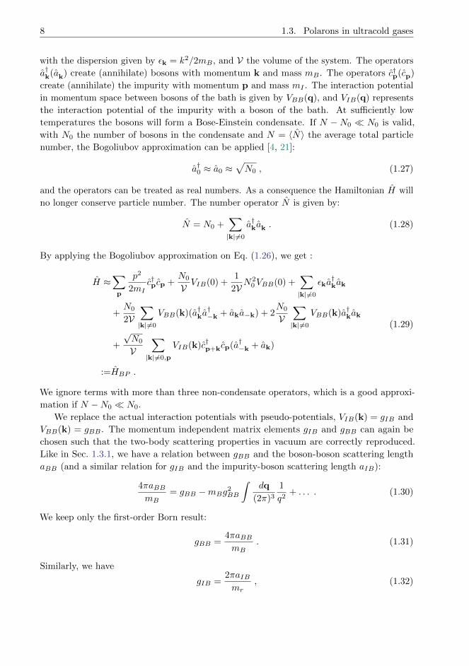
In Fig. 2.12 and Fig. 2.13 we show the contribution of each order to the one-body self-
energy for kFas = 1. At an order Nmax the noise will dominate over the signal given a certain
simulation time. The factorial increase of diagrams will nearly limit Nmax. The different
signs of the diagrams, on the other hand, will have a big impact on Nmax. For example:
the two diagrams that contribute to the third-order self-energy have an opposite sign and
cancel each other almost (see Sec. 2.6). Even though there are only two diagrams, it requires
considerable computational effort to see this cancellation and to calculate ΣN=3(p = 0, τ)
accurately. We observe that ΣN (p = 0, τ) starts oscillating as function of the diagram order
and seems to diverge. For orders larger than 9, ΣN (p = 0, τ) has a bad signal-to-noise ratio,
due to our finite simulation time, and therefore we do not go beyond Nmax.
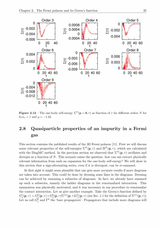
Chapter 2. The Fermi polaron and its Green’s function 35
-0.006
-0.004
-0.002
0
0 20 40
Σ(τ
)
τ
Order 3
-0.0004
0
0.0004
0.0008
0 20 40
Σ(τ
)
τ
Order 4
-0.004
-0.002
0
0 20 40 60
Σ(τ
)
τ
Order 5
0
0.002
0.004
0 20 40 60
Σ(τ
)
τ
Order 6
-0.009
-0.006
-0.003
0
0 20 40 60
Σ(τ
)
τ
Order 7
0
0.003
0.006
0 20 40 60
Σ(τ
)
τ
Order 8
-0.012
-0.008
-0.004
0
0 20 40 60
Σ(τ
)
τ
Order 9
Figure 2.12 – The one-body self-energy ΣN (p = 0, τ) as function of τ for different orders N for
kF as = 1 and µ = −1.22.
2.8 Quasiparticle properties of an impurity in a Fermi
gas
This section contains the published results of the 3D Fermi polaron [28]. First we will discuss
some relevant properties of the self-energies ΣN (p, τ) and ΠN (p, τ), which are calculated
with the DiagMC method. In the previous section we observed that ΣN (p, τ) oscillates and
diverges as a function of N . This scenario raises the question: how can one extract physically
relevant information from such an expansion for the one-body self-energy? We will show in
this section that a sign-alternating series, even if it is divergent, can be re-summed.
At first sight it might seem plausible that one gets more accurate results if more diagrams
are taken into account. This could be done by dressing some lines in the diagrams. Dressing
can be achieved by summing a subseries of diagrams. In fact, we already have summed
up such a subseries, namely the ladder diagrams in the renormalized interaction. This
summation was physically motivated, and it was necessary in our procedure to renormalize
the contact interaction. Let us give another example. Take the Green’s function defined by
G1↓(p, τ) = G0
↓(p, τ)+G0↓(p, τ)Σ(1)(p, τ)G1
↓(p, τ) (see Sec. 2.4 for the definition of Σ(1)(p, τ)).
Let us call G0↓ and Γ0 the ‘bare propagators’. Propagators that include more diagrams will

36 2.8. Quasiparticle properties of an impurity in a Fermi gas
-0.016
-0.012
-0.008
-0.004
0
0.004
0.008
0.012
0.016
0 20 40 60
Σ(τ
)
τ
Order 9Order 8Order 7Order 6Order 5Order 4Order 3
Figure 2.13 – The one-body self-energy ΣN (p = 0, τ) as function of τ for different orders N for
kF as = 1 and µ = −1.22.
Figure 2.14 – The upper diagram shows a fourth-order Σ-diagram which contains a first-order
subdiagram in the dashed circle. In the lower diagram the G0↓-propagators are replaced by G1
↓-
propagators (bold lines) and the upper diagram is included implicitly.

Chapter 2. The Fermi polaron and its Green’s function 37
be called dressed or bold propagators. In the DiagMC simulation we could for example
replace all G0↓ with the dressed G1
↓. From Fig. 2.14 it is clear that diagrams which contain a
first-order diagram as a subdiagram have to be excluded to avoid double counting. In this
way an infinite subset of diagrams is included in each diagram in an implicit way.
We will discuss more advanced schemes and see that taking into account more diagrams
does not always lead to better and more accurate results. We will look at different schemes to
calculate the ground-state properties for the polaron and the molecule to check the robustness
of the results.

Quasiparticle properties of an impurity in a Fermi gas
Jonas Vlietinck1, Jan Ryckebusch1, and Kris Van Houcke1
1Department of Physics and Astronomy, Ghent University, Proeftuinstraat 86, 9000 Gent, Belgium
Abstract
We report on a study of a spin-down impurity strongly coupled to a spin-up Fermisea (a so-called Fermi polaron) with the diagrammatic Monte-Carlo (DiagMC) technique.Conditions of zero temperature and three dimensions are considered for an ultracoldatomic gas with resonant interactions in the zero-range limit. A Feynman diagrammaticseries is developed for the one-body and two-body propagators providing informationabout the polaron and molecule channel respectively. The DiagMC technique allowsus to reach diagram orders that are high enough for extrapolation to infinite order.The robustness of the extracted results is examined by checking various resummationtechniques and by running the simulations with various choices for the propagatorsand vertex functions. It turns out that dressing the lines in the diagrams as much aspossible is not always the optimal choice. We also identify classes of dominant diagramsfor the one-body and two-body self-energy in the region of strong interaction. Thesedominant diagrams turn out to be the leading processes of the strong-coupling limit.The quasiparticle energies and Z-factor are obtained as a function of the interactionstrength. We find that the DiagMC results for the molecule and polaron properties arevery similar to those obtained with a variational ansatz. Surprisingly, this variationalansatz gives very good predictions for the quasiparticle residue even when this residueis significantly smaller than one.
1 Introduction
The notion of a ‘bare’ particle loses its significance once it is strongly coupled to a medium.Landau introduced the notion of a quasiparticle whose properties may be very different fromthose of a bare particle [1]1. The most prominent example is an electron moving in a crystal:the electron displaces the nearby ions and carries this distortion with it. The presence ofthe phonon cloud changes the mass and energy of the electron, that is dubbed as ‘polaron’[2]. More generally, a polaron arises whenever a quantum impurity is strongly coupled to anenvironment. These quantum-mechanical quasiparticles play a key role in the low-energybehavior of a macroscopic quantum liquid.
In recent years, the field of ultracold atoms has provided an exciting framework for studyingpolaronic effects. A key idea is that models designed for describing the rich and non-trivialstructure of the solid state, can be emulated in a clean and controllable manner with ultracoldatoms. For example, so-called Fermi polarons [3, 4, 5], spin-down impurities that are strongly
1The references of the citations in this text are located at the end of this chapter
38 2.8. Quasiparticle properties of an impurity in a Fermi gas

coupled to a spin-up Fermi sea, can be created in a degenerate two-component atomicFermi gas when going to the limit of strong spin-imbalance close to a Feshbach resonance.The impurity is coherently dressed with particle-hole excitations of the Fermi sea. Theproperties of the Fermi polaron are important for the quantitative understanding of a stronglyimbalanced Fermi gas [6].
In this paper, we focus on the ‘attractive Fermi polaron’, with an attractive interactionbetween the impurity and the fermions of the bath. A recent experiment using an ultracoldgas of 6Li atoms in three dimensions revealed the existence of Fermi polarons through anarrow quasiparticle peak in the impurities’ radio-frequency (rf) spectrum [4]. At a criticalinteraction strength, the disappearance of this peak was interpreted as a transition frompolaronic to molecular binding, when the impurity and an atom of the sea form a two-body bound state. Such a transition had theoretically been predicted in three dimensions(3D) by Prokof’ev and Svistunov [3]. To determine the transition point, they developeda diagrammatic Monte Carlo technique (DiagMC) capable of solving the Fermi polaronmodel[3, 8]. Calculations of the ground-state energy showed that for a sufficiently strongattraction between the impurity atom and the atoms of the spin-up Fermi sea, a molecularstate becomes energetically favorable. The crossing point was found at an interaction strength(kFa)c = 1.11(2), with kF the Fermi momentum of the spin-up sea and a the s-wave scatteringlength. A variational treatment developed by Chevy based on an expansion up to singleparticle-hole excitations on top of the unperturbed Fermi sea turned out to be remarkablyaccurate [9]. A combination of Chevy’s ansatz with a variational wave function in themolecular limit [10, 11, 12] also revealed the polaron-to-molecule transition, very close to theDiagMC result.
In the present work, we study the quasiparticle properties of the Fermi polaron problemin 3D with the DiagMC technique [3, 8]. This technique evaluates a series of Feynmandiagrams for the one-particle and two-particle proper self-energies. A full description ofthe DiagMC algorithm was presented in Ref. [8]. Building on the work of Ref. [8] we haveimplemented the DiagMC algorithm independently. We explore various DiagMC schemes[13] and series resummation methods to check the robustness of the results against thepossible uncertainties of summing the series. First, we confirm the transition point. Next, wecalculate the quasiparticle residue which we compare to experimental data and variationalresults. The quasiparticle residue, or Z-factor, gives the overlap of the non-interacting wavefunction and the fully interacting one,
Zp = |〈ΨN↑0 |0↓, FS(N↑)〉|2 , (1)
with |ΨN↑0 〉 the fully interacting ground state and |0↓, FS(N↑)〉 a free spin-down atom carrying
momentum p = 0 in a non-interacting Fermi sea FS of N↑ spin-up atoms. The spin-upatoms are non-interacting since p-wave scattering is negligible. The residue reflects theimpurity’s probability of free propagation.
The outline of the paper is as follows. In Section 2 we introduce the model and the structureof the Feynman diagrammatic expansion. In Section 3 we discuss the results of the numericalcalculations. Thereby, we investigate on how the results depend on the choices made withregard to the diagrammatic series, like the use of bare versus dressed propagators. Alsothe resummation of the diagrammatic series is discussed in depth. The results for thequasiparticle properties, like the residue, are the subject of Section 4.
Chapter 2. The Fermi polaron and its Green’s function 39

2 Model and Diagrammatic structure
We consider a dilute two-component gas of ultra-cold fermionic atoms interacting via thevan der Waals-potential. The Hamiltonian has a kinetic and interaction term
H =∑
k,σ=↑↓εkσ c
†kσ ckσ +
1
V∑
k,k′,q
V (k− k′) c†k+ q
2 ↑c†−k+ q
2 ↓c−k′+ q
2 ↓ck′+ q
2 ↑.
The operators c†kσ (ckσ) create (annihilate) fermions with momentum k and spin σ. Thespin-σ fermions have mass mσ and dispersion εkσ = k2/2mσ, and V is the volume ofthe system. We take ~ = 1 throughout the paper, and consider the mass-balanced casem↑ = m↓ = m. All the theoretical considerations are for zero temperature (or T TF withTF the Fermi temperature). The diluteness of the system ensures that the range b of thepotential is much smaller than the typical inter-particle distance 1/kF , or kF b 1, withkF the Fermi momentum of the spin-up sea, and therefore the details of the interactionpotential become irrelevant. Accordingly, without loss of generality, one can model theshort-ranged interaction as a contact interaction, V (r) = g0δ(r), in combination with thestandard ultra-violet divergence regularization procedure described below.
The one-body and two-body propagators provide access to information about the ‘polaron’and ‘molecule’ channel respectively. The polaron and molecule are two distinct objectsbelonging to different charge sectors. The one-body and two-body propagators are discussedin Sections 2.1 and 2.3. The adopted regularization procedure for the renormalized interactionis the subject of Section 2.2. The DiagMC method is introduced in Section 2.4.
2.1 One-body propagator
The polaron quasiparticle properties can be extracted from the impurity’s Green’s functiondefined as
G↓(k, τ) = −θ(τ)〈ΦN↑0 |ck↓(τ)c†k↓(0) |ΦN↑
0 〉 , (2)
with ck↓(τ) the annihilation operator in the Heisenberg picture,
ck↓(τ) = e(H−µN↓−µ↑N↑)τ ck↓e−(H−µN↓−µ↑N↑)τ . (3)
The propagator G↓(k, τ) is written in the momentum imaginary-time representation, µ is
a free parameter, Nσ is the number operator for spin-σ particles, and µ↑ is the chemicalpotential of the spin-up sea. The state
|ΦN↑0 〉 = |〉↓|FS(N↑)〉 , (4)
consists of the spin-down vacuum and the non-interacting spin-up Fermi sea. Since weare dealing with an impurity spin-down atom, G↓ is only non-zero for times τ > 0. Theground-state energy and Z-factor can be extracted from the Green’s function of Eq. (2).
Inserting a complete set of eigenstates |ΨN↑n 〉 of the full Hamiltonian (2) for one spin-down
40 2.8. Quasiparticle properties of an impurity in a Fermi gas

particle and N↑ spin-up particles into Eq. (2) yields for k = 0
G↓(0, τ) = −θ(τ)∑
n
|〈ΨN↑n |c†0↓|Φ
N↑0 〉|2e−(En(N↑)−EFS−µ)τ
τ→+∞= −Zp e−(Ep−µ)τ ,
with Ep the energy of the polaron, En(N↑) the energy eigenvalues of the Hamiltonian (2)and EFS = 3 εFN↑/5 the energy of the ideal spin-up Fermi gas, with εF = k2
F /(2m) theFermi energy.
The difference between the polaronic and molecular state is embedded in the factors
|〈ΨN↑n |c†0↓|Φ
N↑0 〉|2 in Eq. (5). For situations where the polaron is a well-defined quasiparticle in
the ground state |ΨN↑0 〉, we have Eq. (1) for the Z-factor and Ep = E0(N↑)−EFS . If, on the
other hand, the ground state |ΨN↑0 〉 is a dressed molecule the overlap 〈ΨN↑
0 |c†0↓|ΦN↑0 〉 is zero
[11]. This is clear from the expansion of the molecular state in the number of particle-holeexcitations,
|ΨN↑0 〉 =
(∑′
k
ξkc†−k↓c
†k↑ +
∑′
k,k′,q
ξkk′qc†q−k−k′↓c
†k↑c†k′↑cq↑ + . . .
)|ΦN↑−1
0 〉 . (5)
The coefficients ξ are variational parameters, and the primes indicate that the sums on k,k′ and q are restricted to |k|, |k′| > kF and |q| < kF . Even if a molecule is formed in theground state, the polaron can be a well-defined excited state (in the sense of a narrow peakin the spectral function), and Zp can be non-zero.
For vanishing interactions V the impurity Green’s function of Eq. (2) becomes
G0↓(k, τ) = −θ(τ)e−(εk↓−µ)τ . (6)
The one-body propagator for the spin-up sea is defined as
G↑(k, τ) = −〈ΨN↑0 |Tτ
[ck↑(τ)c†k↑(0)
]|ΨN↑
0 〉 , (7)
with Tτ the time-ordering operator. Without interactions, one obtains the free propagator
G0↑(k, τ) =
−e−(εk↑−εF )τθ(|k| − kF ) if τ > 0 ,
e−(εk↑−εF )τθ(kF − |k|) if τ < 0 .
Our goal is to calculate the G↓ of Eq. (2) to extract Ep by means of Eq. (5). This isachieved by summing all irreducible one-particle self-energy diagrams with the DiagMCalgorithm (which works in momentum-imaginary-time representation). The irreducible self-energy Σ(k, ω) in imaginary-frequency representation is obtained after a numerical Fouriertransform, and inserted into Dyson’s equation to give G↓,
[G↓(k, ω)
]−1=[G0↓(k, ω)
]−1 − Σ(k, ω) , (8)
with ω the imaginary frequency. A graphical representation of the Dyson equation is shownin the top panel of Fig. 1. As was shown in Ref. [8], the polaron energy Ep and Z-factor Zp
Chapter 2. The Fermi polaron and its Green’s function 41

= +
= +
Σ
Π
G G0
Γ Γ0
Figure 1 – Graphical representation of the Dyson equation and the Bethe-Salpeter equation. Thefree (dressed) one-body impurity propagator is denoted by G0
↓ (G↓). The Σ and Π are the one-bodyand two-body self-energies, respectively. The Γ is the fully dressed interaction, wheres Γ0 is thepartially dressed interaction obtained by summing all the bare ladders G0
↓G0↑ (see Eqs. (14) and
(15)).
can be extracted directly from the self-energy Σ(0, τ),
Ep =
∫ +∞
0
dτ Σ(0, τ) e(Ep−µ)τ , (9)
Zp =1
1−∫ +∞
0dτ τ Σ(0, τ) e(Ep−µ)τ
. (10)
The effective mass m∗ of the polaron is evaluated with the estimator[8]
m∗ =1/Zp
1/m+B0, (11)
with
B0 =
∫ +∞
0
dτ e(Ep−µ)τ
[1
3∇2
kΣ(k, τ)|k=0
], (12)
which can conveniently be estimated by expanding Σ(k, τ) in Legendre polynomials. Oneobtains
1
3∇2
kΣ(k, τ)|k=0 =15
2∆3
∫ ∆
0
dk Σ(k, τ)
(3k2
∆2− 1
), (13)
and the integral can be evaluated during the MC simulation. The upper limit of integration(∆) is optimized to minimize the statistical noise while avoiding a systematic error at toolarge ∆. We also used an alternative way by calculating the quasiparticle spectrum E(k)and fitting m∗ via E(k) = Ep + k2/(2m∗).
2.2 Renormalized interaction
We introduce the s-wave scattering length a for collisions between spin-up and spin-downparticles. One of the advantages of working with Feynman diagrams is that one can workdirectly in the zero-range limit kF b→ 0 (or, equivalently, Λ/kF → +∞ with Λ an ultravioletmomentum cut-off) while keeping kFa constant. Thereby, the ultra-violet physics can betaken into account by means of a summation over all Feynman ladder diagrams.
42 2.8. Quasiparticle properties of an impurity in a Fermi gas

In momentum-imaginary-frequency representation (p,Ω), one obtains for the partially dressedinteraction
Γ0(p,Ω) = g0 + g0 Π0(p,Ω) Γ0(p,Ω) , (14)
with Π0 the two-particle self-energy consisting of one ‘bare’ ladder
Π0(p,Ω) = − 1
2πV∑
|q|<Λ
∫dω G0
↑(p
2+ q, ω)G0
↓(p
2− q,Ω− ω)
=1
V∑
|q|<Λ
θ(|p/2 + q| − kF )
iΩ− p2/(4m)− q2/m+ µ+ εF,
(15)
where the momentum cutoff Λ is required to keep the sum finite. The bare coupling constantV (p) =
∫dre−ip·rV (r) = g0 can be eliminated in favor of the physical scattering length a by
using standard scattering theory
1
g0=
m
4πa− 1
V∑
|k|<Λ
1
2εk. (16)
The Γ0(p,Ω) from Eq. (14) can be expressed in terms of the s-wave scattering length a, bytaking the limit Λ→ +∞ and g0 → 0− with a fixed. In this zero-range limit, one gets
[Γ0(p,Ω)]−1 = [Γ0(p,Ω)]−1 − Π(p,Ω) , (17)
with
Π(p,Ω) = −∫
dq
(2π)3θ(kF − q)
1
iΩ− q2
2m −(p−q)2
2m + µ+ εF. (18)
Here, we have taken the thermodynamic limit (V → +∞ and N↑/V fixed). The integral inEq. (18) can be evaluated analytically, and the dressed interaction in vacuum is given by
[Γ0(p,Ω)]−1 =m
4πa− m
8π
√p2 − 4m(iΩ + µ+ εF ) , (19)
for Ω 6= 0 or µ < −εF , and assuming the principal branch. For µ < −[εF + 1/(ma2)], theFourier transform to imaginary time can be done analytically, producing
Γ0(p, τ) = − 4π
m3/2e−( p
2
4m−µ−εF )τ
(1√πτ
+1√ma
eτ
ma2 erfc(−√τ
m
1
a
)), (20)
with erfc(x) the complementary error function. As in Ref. [8], we use Γ0(p, τ) as a partiallydressed interaction vertex in the diagrammatic series, instead of the bare interaction vertexg0. This dressed vertex is calculated here in imaginary time representation by performingthe Fourier transform of Eq. (17) numerically.
In a next step, the interaction vertex will be fully dressed by calculating the two-particleself-energy Π and plugging it into the Bethe-Salpeter equation,
[Γ(p,Ω)]−1 = [Γ0(p,Ω)]−1 −Π(p,Ω) . (21)
A graphical representation of this equation is shown in Fig. 1. The self-energy Π containsall connected two-particle diagrams that are irreducible with respect to cutting a single Γ0
propagator. To avoid double counting, the diagrams for Π should not contain any ladders,since those have been summed in Γ0 by means of the Eq. (14). This rule also holds whensumming diagrams for the one-body self-energy Σ, built from free propagators G0
σ and Γ0.
Chapter 2. The Fermi polaron and its Green’s function 43

2.3 Two-body propagator
Here, we consider the pair annihilation operator,
Pk =∑
q
ϕ(q) ck−q↑cq↓ , (22)
with ϕ(q) the momentum representation of the wave function ϕ(r) for relative motion of thetwo fermions of opposite spin. The two-particle propagator is defined as
G2(k, τ) = −θ(τ)〈ΦN↑0 |Pk(τ)P †k(0) |ΦN↑
0 〉 , (23)
where we included the fact that the impurity spin-↓ atom propagates forward in time.
Inserting the complete basis |ΨN↑+1n 〉 for (N↑ + 1) spin-up particles and one spin-down
particle, gives
G2(0, τ) = −θ(τ)∑
n
|〈ΨN↑+1n |P †0 |Φ
N↑0 〉|2e−(En(N↑+1)−EFS(N↑)−µ↑−µ)τ
τ→+∞= −Zmol e
−(Emol−µ)τ ,
(24)
with Emol the molecule energy and Zmol the molecule Z-factor. If the molecule is a well-defined quasiparticle in the ground state, we have
Zmol = |〈ΨN↑+10 |P †0 |Φ
N↑0 〉|2 , (25)
and Emol = E0(N↑ + 1)− EFS(N↑)− µ↑. Note that the value of Zmol depends on the wavefunction ϕ(q). The functional from of this pair wave function depends on the nature ofexperiment used to probe the molecule.
In practice, it is easier to calculate the molecule energy from the fully dressed interaction Γ(see Eq. (21)). This function is closely related to the pair correlation function, namely,
Γ(k, τ) = g0δ(τ) + g0 P(k, τ) g0 , (26)
withP(r, τ) = −θ(τ)〈ΦN↑
0 |(Ψ↑Ψ↓)(r, τ)(Ψ†↓Ψ†↑)(0, 0)|ΦN↑
0 〉 , (27)
the pair correlation function. The field operators Ψ†σ(r) =∑
k e−ikrc†k,σ/
√V create a spin-σ
fermion at position r. In Eq. (27) the pair of particles is created at the same position (whichcorresponds to ϕ(q) = 1 in Eq. (22)). The structure of the fully dressed interaction Γ andthe two-particle propagator G2 now implies that both structures have the same poles (seeEq. (26)). Therefore, the exponential tail of the function Γ(k = 0, τ) can conveniently beused for estimating the molecule energy, rather than the tail of G2(0, τ). This is equivalentwith looking for this pole of the Bethe-Salpeter equation (21). The molecule’s energy Emol isgiven by the parameter µ that satisfies the equation
[Γ0(p = 0,Ω = 0)]−1 = Π(p = 0,Ω = 0) , (28)
where the left-hand-side is known analytically, and the right-hand-side is evaluated with theDiagMC algorithm in imaginary-time domain.
44 2.8. Quasiparticle properties of an impurity in a Fermi gas

2.4 Diagrammatic Monte Carlo
DiagMC evaluates the series of Feynman diagrams for the self-energy in a stochastic way.We deal with both the one-body and two-body self-energies. In a first step, the self-energy isbuilt from the free propagators G0
σ and the partially dressed interaction Γ0 (obtained throughsummation of G0
↓G0↑ ladders; as discussed in Section 2.2). We will refer to this series as the
‘bare series’. Fig. 2 shows the one-body and two-body self-energy diagrams up to order 3in the bare scheme. The order of a diagram is N when there are N dressed interactions Γ(i.e., N boxes) present in the Σ-diagram, and N − 1 boxes in the Π-diagram. Note that thediagrams cannot contain ladders since these have been taken into the vertex function Γ0. Toillustrate the factorial growth with order, the number of one-body self-energy diagrams forgiven order N ≤ 12 is given in the second column of Table 1 for the bare series.
In a second step, we will use dressed propagators or ‘bold lines’ in the diagrams. Such dressed(skeleton) series are evaluated with the Bold DiagMC technique [13, 3]. We consider the casewith only dressed G↓ propagators while keeping Γ0 of Eqs. (17) and (18) as renormalizedinteraction, and the case whereby both the one-body propagators and interactions are dressed.We will refer to these skeleton series as ‘bold G’ and ‘bold G-Γ’, respectively. In the lattercase, the Bold DiagMC algorithm is constructed as follows: given approximate one-body andtwo-body self-energies Σ and Π, the Dyson and Bethe-Salpeter equation are solved to deliverthe one-body propagator G↓ and the dressed interaction Γ (see Eqs. (8) and (21)). In a nextstep, these are used to dress the series for Σ and Π, which are evaluated stochastically withDiagMC up to order N∗. This self-consistent cycle is repeated until convergence is reached.Fig. 3 shows the skeleton (bold G-Γ) series for the one- and two-body self-energies up toorder 4. Evidently, when dressing the lines in the self-energies, one has to keep track oftwo-particle reducibility, and systematically avoid any double counting. This typically meansthat at any order N the numbers in the second column of Table 1 (Bare) are an upper limitof the number of diagrams in the third and fourth column. At N = 2 and N = 4, however,the number of diagrams increases due to the fact that ladders should be included again onceG↓ is bold. All the diagrams of Table 1 are summed explicitly during the (Bold) DiagMCsimulation.
3 Resummation and boldification
When considering a diagrammatic series, it is natural to ask whether there are dominantclasses of diagrams. Identification of the dominant diagrams potentially allows one to makegood approximations. To address this issue, we constructed a histogram counting how manytimes a certain topology is sampled. We consider first the bare series. It turns out thatfor the one-body self-energy, roughly half of the simulation time is spent on sampling twodiagrams at each order. These two diagrams are shown in Figure 4 for diagram order six.To understand why these two diagrams are dominant at a fixed N , we use an argumentfirst made by Hugenholtz[14]. For the dilute spin-up gas, momentum integration inside theFermi sea is heavily restricted in phase space (momentum integration runs up to the Fermimomentum kF ∼ (N↑/V)1/3). This implies the presence of a backward (or hole) spin-uppropagator reducing the contribution of the diagram significantly, while the forward (particle)propagator enhances the contribution roughly with a factor
∫|k|>kF dk. As a consequence,
Chapter 2. The Fermi polaron and its Green’s function 45

N Bare Bold G Bold G-Γ1 1 1 12 0 1 03 2 2 14 6 7 25 34 34 136 210 206 747 1,526 1,476 5448 12,558 12,123 4,4589 115,618 111,866 41,22110 1,177,170 1,143,554 421,41211 13,136,102 12,816,572 4,722,88112 159,467,022 156,217,782 57,553,440
Table 1 – Factorial increase of the number of Feynman diagrams. At fixed order N , the numberof one-body self-energy diagrams is given for different types of series: the bare series, the skeletonseries with dressed G↓ (bold G), and the skeleton series with dressed G↓ and Γ lines (bold G-Γ).
+=
+ + ...
= +
+ + ...
Σ
Π
Figure 2 – Diagrammatic expansion for the one-body self-energy Σ and the two-body self-energyΠ. Here, the diagrams are built from the bare propagators G0
σ (thin lines), and the partially dressedinteraction Γ0 (light grey box). All diagrams have a ‘backbone’ structure, since we have a singleimpurity propagating forward in time and interacting with a Fermi sea of free particles.
46 2.8. Quasiparticle properties of an impurity in a Fermi gas

!"
!#$$$!
!
" !!
! !#$$$
!
Σ
Π
Figure 3 – Skeleton diagrammatic expansion for the one-body and two-body self-energy: theimpurity propagator and interaction lines that appear in the diagram are fully dressed solutions ofthe Dyson equation and the Bethe-Salpeter equation (see Fig. 1).
Figure 4 – The figure contains the two dominant one-body self-energy diagrams for N = 6.Imaginary time runs from right to left.
Chapter 2. The Fermi polaron and its Green’s function 47
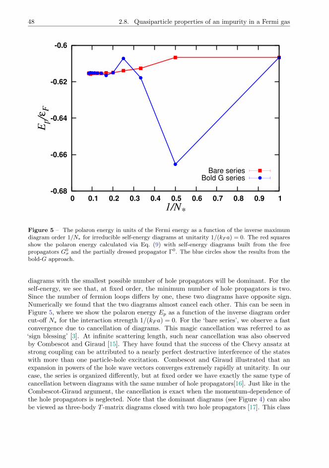
-0.68
-0.66
-0.64
-0.62
-0.6
0 0.1 0.2 0.3 0.4 0.5 0.6 0.7 0.8 0.9 1
Ep/εF
1/N*
Bare series
Bold G series
Figure 5 – The polaron energy in units of the Fermi energy as a function of the inverse maximumdiagram order 1/N∗ for irreducible self-energy diagrams at unitarity 1/(kF a) = 0. The red squaresshow the polaron energy calculated via Eq. (9) with self-energy diagrams built from the freepropagators G0
σ and the partially dressed propagator Γ0. The blue circles show the results from thebold-G approach.
diagrams with the smallest possible number of hole propagators will be dominant. For theself-energy, we see that, at fixed order, the minimum number of hole propagators is two.Since the number of fermion loops differs by one, these two diagrams have opposite sign.Numerically we found that the two diagrams almost cancel each other. This can be seen inFigure 5, where we show the polaron energy Ep as a function of the inverse diagram ordercut-off N∗ for the interaction strength 1/(kFa) = 0. For the ‘bare series’, we observe a fastconvergence due to cancellation of diagrams. This magic cancellation was referred to as‘sign blessing’ [3]. At infinite scattering length, such near cancellation was also observedby Combescot and Giraud [15]. They have found that the success of the Chevy ansatz atstrong coupling can be attributed to a nearly perfect destructive interference of the stateswith more than one particle-hole excitation. Combescot and Giraud illustrated that anexpansion in powers of the hole wave vectors converges extremely rapidly at unitarity. In ourcase, the series is organized differently, but at fixed order we have exactly the same type ofcancellation between diagrams with the same number of hole propagators[16]. Just like in theCombescot-Giraud argument, the cancellation is exact when the momentum-dependence ofthe hole propagators is neglected. Note that the dominant diagrams (see Figure 4) can alsobe viewed as three-body T -matrix diagrams closed with two hole propagators [17]. This class
48 2.8. Quasiparticle properties of an impurity in a Fermi gas

-4.3
-4.2
-4.1
-4
-3.9
-3.8
-3.7
0 0.1 0.2 0.3 0.4 0.5 0.6 0.7 0.8 0.9 1
Ep/εF
1/N*
Bare series
Bold G series
Figure 6 – Same plot as Figure 5, but now considering the interaction strength parameter1/(kF a) = 1.333. In the bare series, small oscillations prevent us from extrapolating to infinitediagram order.
of diagrams, in which there are at most two particle-hole excitations, has been consideredpreviously for the polaron problem [12, 15]. It was shown that they exactly reproduce theSkorniakov and Ter-Martirosian equation [18] in the BEC limit. In this strong-couplinglimit, the dominant process is scattering between a dimer and a spin-up fermion, which isdiagrammatically represented by the three-body T-matrix diagrams. Away from this limit,the considered class of diagrams turns out to give a quantitatively good correction to thelowest order result. We find that this is due to their dominance, even away from the BEClimit.
When going towards the BEC side (1/a > 0), the cancellation between dominant diagramsof the type shown in Figure 4 is no longer perfect. Figure 6 shows the polaron energy as afunction of 1/N∗ for 1/(kFa) = 1.333. For the bare series, the oscillations prevent one fromextracting Ep for 1/N∗ → 0.
To cure the bad convergence of the bare series for 1/(kFa) > 0 one can include more diagramsby dressing the propagators. We start by dressing the spin-down propagator lines, whilekeeping the partially dressed Γ0. Diagrams reducible with respect to cutting two spin-downlines should no longer be sampled, since they are included implicitly. For 1/(kFa) = 0 theself-energy Σ(k, τ) converges in this ‘bold G scheme’ for N∗ ≥ 7. Extrapolation to infinite N∗gives the exact Σ and G↓. Figure 5 includes the polaron energy as function of diagram order
Chapter 2. The Fermi polaron and its Green’s function 49

cut-off when the one-body self-energy is built with the exact G↓. The bare and bold seriesconverge to the same energy. Remarkably, the dressed scheme gives worse results at lowN∗. This indicates that approximations based on a few low order diagrams are completelyuncontrolled, and including more diagrams by dressing the lines does not necessarily improvethe quality of the results.
For 1/(kFa) = 1.333, we see that dressing the impurity lines helps to get rid of the residualoscillations in the bare scheme (see Figure 6). One might expect that dressing even more,by using a fully dressed Γ instead of Γ0, might lead to even better convergence. Figure 7shows however that, even for 1/(kFa) = 0, the fully bold series (bold G-Γ scheme) doesnot seem to converge (N∗ is the diagram cut-off for both Σ and Π, and a Bold DiagMCsimulation is done for each N∗), in contrast to the results of Ref.[8]. The data for the fullybold simulation of Ref.[8] was obtained by using the exact G and Γ (i.e. extrapolated to theN∗ → ∞ limit with resummation factors). They were not obtained with a self-consistentsimulation, which explains the difference. Moreover, data is not shown above N∗ = 7, whereoscillations do occur. In order to understand why the series no longer converges, we introducean intermediate scheme (which we call bold G-Γ1): the self-energy is built from the fullyconverged G↓ and a partially dressed interaction Γ1, built from summing the ladders G↓G0
↑.The result is also shown in Figure 7, and we again observe convergence to the same answeras in Figure 5. The key difference between both schemes is that in the bold G-Γ1 scheme,both dominant diagrams shown in Fig. 4 still explicitly contribute to the self-energy, whereasin the fully bold scheme the upper dominant diagram becomes reducible and is taken intoaccount self-consistently. This means that the balance of cancellation between diagrams isbroken, and a single dominant diagram keeps contributing at each order. So, it turns outthat dressing the diagrams as much as possible is not always a good idea. In this respect,our findings disagree with Ref.[8].
A second method to cure the bad convergence of the bare series on the BEC side, is toemploy series resummation techniques. We will use the Abelian resummation techniques[19]which have been used when calculating the equation of state of the unitary gas with BoldDiagMC[20]. This resummation technique works as follows. One starts from a seriesf(x) =
∑n dnx
n that has a finite radius of convergence R > 0. The idea is to sum the seriesat some point x0 outside of the radius R by analytically continuing the function f . Thisprovides a good procedure for summing the divergent series in the sense that it respects basicoperations (sum, multiplication and derivative) and that it preserves distinctness[19]. It iswell-known that with analytic continuation, one can encounter problems with the existenceand/or uniqueness of the solution[21]. However, one can formally define a domain called the‘Mittag-Leffler star’ where the function can be analytically continued along straight lines[0, x0]. Note that this star will always contain the disk of convergence. It can be shown[19]that for each point x0 of the Mittag-Leffler star, the limit
limε→0+
∑
n
dnxn0 e−ελn , (29)
with λn = n log(n) for n > 0 and λ0 = 0, exists and is equal to the analytic continuation off to the point x0. Note that within the disk of convergence the procedure works equally well,and can improve the rate of convergence. We apply the Abelian resummation technique tothe expansion of the self-energy Σ and Π. As the analytic structure of Σ and Π is unknown,it is currently impossible to determine whether there is a finite radius of convergence and
50 2.8. Quasiparticle properties of an impurity in a Fermi gas

-0.68
-0.66
-0.64
-0.62
-0.6
-0.58
-0.56
0 0.1 0.2 0.3 0.4 0.5 0.6 0.7 0.8 0.9 1
Ep/εF
1/N*
G - Γ1 scheme
bold G - bold Γ scheme
Figure 7 – The polaron energy in units of the Fermi energy as a function of the inverse maximumdiagram order 1/N∗ for irreducible self-energy diagrams at unitarity 1/(kF a) = 0. The blue circlesshow results from a fully Bold DiagMC simulation: the self-energy diagrams are built from fullydressed one-particle propagators G↓ and two-particle propagators Γ up to self-energy diagram orderN∗. The red squares show the polaron energy calculated with diagrams built with the exact G↓ anda partially dressed interaction Γ1 containing the sum of all G↓G
0↑ ladders.
whether we are in the Mittag-Leffler star. In practice, we apply different resummationtechniques (i.e., different functions λn), and test the uniqueness of the result.
We use following λn: (i) Lindelof 1: λn = n log(n) for n > 0 and λ0 = 0; (ii) Lindelof 2:λn = (n − 1) log(n − 1) for n > 1 and λ0 = λ1 = 0; (iii) Gauss 1: λn = n2 for n ≥ 0; (iv)Gauss 2: λn = (n − 1)2 for n ≥ 1 and λ0 = 0; (iv) Gauss 3: λn = (n − 2)2 for n ≥ 2 andλ0 = λ1 = 0. Before applying these resummation techniques to our diagrammatic series,we illustrate its power with an example for the geometric series. Figure 8 shows the sumsfε(x0 = −3) =
∑n x
n0 e−ελn for a few choices of λn. At small ε, the computation of fε is no
longer feasible due to finite computer precision. By extrapolating to ε = 0, we indeed find1/(1− x0) with high precision. The Lindelof curve gives a slighly less accurate extrapolationbecause it suppresses high order contributions in a much smoother fashion than the Gaussianresummation. When applying these techniques to our diagrammatic series, it is the growthof the statistical error bars (due to factorial complexity) that prevents us from going tovery small values of ε. Figure 9 shows the polaron energy calculated with the resummedself-energy as a function of the control parameter ε for 1/(kFa) = 1.333. The polaron energy
Chapter 2. The Fermi polaron and its Green’s function 51

-0.1
0
0.1
0.2
0.3
0.4
0.5
0.6
0.7
0 0.1 0.2 0.3 0.4 0.5
f ε(x0=-3)
ε
Gauss 1
Gauss 2
Lindelof 1
Figure 8 – Illustration of the Abelian resummation technique for the geometric series. We evaluatefε(x0) =
∑n x
n0 e−ελn for x0 = −3. and various choices of λn. The value of the analytically continued
function 1/(1− x0) is retrieved for ε→ 0+.
Ep can be extracted with high accuracy. The major source of error bar stems from theuncertainty in the extrapolation.
Histogramming the different topologies of the two-body self-energies Π revealed a dominantdiagram at each order. This diagram is shown in Figure 10. Again it shows a three-bodyT -matrix structure that is closed with a single spin-up hole propagator. Upon increasingthe diagram order up to 20, we observe a steady growth in the contribution of this diagram.This is illustrated in Figure 11, where we plot the n-th order contribution Πn to the two-body self-energy as a function of imaginary time τ for external momentum zero. Figure 12illustrates that we can nonetheless get accurate values for the molecule energy Emol by usingdifferent Abelian resummation techniques and extrapolating to ε = 0+. Again, the Gaussianresummation methods allow one to reach very small values of ε. The quoted error bars arerather conservative as we include the extrapolated results obtained with all choices for λn.
We also tested the resummability of the fully bold series (bold G - bold Γ scheme), since thiswas used in the Bold DiagMC method for determining the equation of state of the unitarygas[20]. When applying the Abelian resummation techniques and extrapolate to ε = 0+ at1/(kFa) = 0, the correct polaron energy is retrieved. This constitutes an independent checkfor the resummation of the skeleton series.
52 2.8. Quasiparticle properties of an impurity in a Fermi gas

-4.04
-4.03
-4.02
-4.01
-4
-3.99
-3.98
0 0.2 0.4 0.6 0.8 1
Ep/εF
ε
Gauss 1
Gauss 3
Lindelof 1
Figure 9 – Abelian resummation of the bare series of one-body self-energy diagrams at 1/(kF a) =1.333. The polaron energy Ep/εF is extracted in the limit ε = 0+ for different choices of λn.
Figure 10 – At fixed order, there is one dominant diagram for the two-body self-energy. Here, wedraw this diagram at order six.
Chapter 2. The Fermi polaron and its Green’s function 53

-0.015
-0.01
-0.005
0
0.005
0.01
0.015
0 2 4 6 8 10 12
Πn(p=0,τ)
τ
n=2
n=3
n=14
n=15
n=18
n=19
Figure 11 – The two-particle self-energy Π at external momentum zero as a function of imaginarytime for kF a = 1. The Πn are the contribution of all n-th order diagrams, and here shown for variousn. As n increases, Πn keeps on growing. We work in units kF = 1, m = 1, ~ = 1 and µ/εF = −3.2.The noise in the curves indicates the magnitude of the statistical error.
4 Quasiparticle properties
As an independent cross-check of Ref. [3], which uses alternate ways of resumming thediagrammatic series, we calculate the ground-state energies of the polaron and molecule.Figure 13 shows these energies shifted by the vacuum molecule energy Eb = −1/(ma2) inunits of the Fermi energy εF . A selection of the polaron and molecule energies is also givenin Table 2. We find the transition point at (kFa)c = 1.15(3), in agreement with Ref. [3].Close to the transition point, we find polaron energies that differ about 1% with the polaronenergies of Ref.[3], which, we believe, is due to a small systematic error in the lowest orderdiagram in Ref.[3]. The variational energies obtained from a wave-function ansatz for thepolaron[9] and the molecule[11] are very close to the Monte Carlo results. Note that Chevy’svariational ansatz for the polaron state is completely equivalent with the non-self-consistentT -matrix approximation [12] which is exactly our bare series at N∗ = 1. Fixed node-difussionMonte Carlo (FN-DMC) results are also in good agreement with the DiagMC data. For1/(kFa) = 2 it seems that systematic errors on the FN-DMC results were underestimated,since FN-DMC should in principle give an upper bound to the true ground-state energy.
Figure 14 shows the effective mass of the polaron as calculated with DiagMC. We compare
54 2.8. Quasiparticle properties of an impurity in a Fermi gas

-2.66
-2.62
-2.58
-2.54
0 0.2 0.4 0.6 0.8 1
Emol/
εF
ε
Gauss 1
Gauss 2
Gauss 3
Lindelof 1
Lindelof 2
Figure 12 – Abelian resummation of the bare series of two-particle self-energy diagrams at kF a = 1.The molecule energy Emol/εF is extracted in the limit ε = 0+ for different choices of λn.
with the ENS experiment [5] at unitarity, DiagMC calculations by Prokof’ev-Svistunov[3],FN-DMC[6, 7], a variational calculation up to two particle-hole excitations[12], and the firstorder (N∗ = 1) result in the bare scheme and the fully bold G-Γ scheme. The experimentaleffective mass, which is in perfect agreement with DiagMC [3], was extracted from the lowfrequency breathing modes, and in particular the Fermi polaron breathing mode. The lowestorder bare calculation, also known as T -matrix approximation, is equivalent to the Chevyansatz, while the lowest order bold calculation corresponds to the self-consistent T -matrixapproximation. These results show that including only single particle-hole pair excitions doesnot lead to accurate results for the effective mass, while the variational calculation basedon diagrams taking into account at most two particle-hole pairs excitations agrees with theDiagMC results[12].
Experimental and theoretical quasiparticle residues are shown in Fig. 15. To create andprobe polarons, the MIT experiment[4] starts from a cloud of 6Li atoms with most atomsoccupying the lowest hyperfine state |1〉 (spin-up), and about 2% of the atoms occyping thehyperfine state |3〉 (spin-down) in the degenerate regime T ≈ 0.14 TF with TF the Fermitemperature. A broad Feshbach resonance is used to enhance the scattering between atomsin states |1〉 and |3〉. Radio-frequency (rf) spectra of the spin-up and spin-down componentsare measured. The atoms are transferred to a third empty state with very weak final-stateinteractions. Therefore, the measured transition rate I can be connected with the impurity’s
Chapter 2. The Fermi polaron and its Green’s function 55

-0.8
-0.6
-0.4
-0.2
0
0.2
-0.5 0 0.5 1 1.5 2
(E-E
b)/
εF
1/kFa
Polaron DiagMC-this workMolecule DiagMC-this work
Chevy’s ansatzMolecular ansatz
FN-DMCProkof’ev-SvistunovProkof’ev-Svistunov
Figure 13 – The extracted polaron and molecule energy as a function of the interaction strength1/(kF a). The energies are expressed as (E − Eb)/εF , with Eb = −1/(ma2) the molecule energy invacuum. The FN-DMC results are from Ref.[6], the variational results for the polaron from Ref.[9]and for the molecule from Ref.[11]. DiagMC results by Prokof’ev and Svistunov[3] are also shown.
spectral function ρ↓ in linear response theory[22, 23]
I(ωL) ∝∑
k
nF (εk − µ− ωL) ρ↓(k, εk − µ− ωL) , (30)
with ωL the frequency of the rf photons and nF (x) = 1/(1+eβx) the Fermi distribution. Notethat the spectral function depends on the temperature. Density inhomogeneities are takencare of through tomographic reconstruction [4]. At sufficiently weak attractions, the Fermipolaron is observed as a narrow peak in the impurity spectrum that is not matched by thebroad environment spectrum. The peak position gives the polaron energy Ep, and was foundto be in perfect agreement with the DiagMC results of Ref. [3]. The polaron Z-factor wasmeasured by determining the ratio of the area under the impurity peak that is not matchedby the environment, and the total area under the impurity’s spectrum. The experimentalZ-factor from Ref. [4] is shown in Figure 15, together with the Z-factor calculated fromChevy’s ansatz[11, 24], the fully self-consistent result in lowest order (N∗ = 1) and ourDiagMC simulation. DiagMC data for the Z-factor is also given in Table 2.
The results obtained via DiagMC simulation agree extremely well with Chevy’s variationalansatz. This is very surprising in the strongly interacting regime where Zp is significantly
56 2.8. Quasiparticle properties of an impurity in a Fermi gas
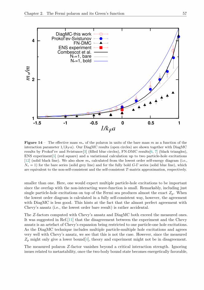
1
2
4
-1.5 -1 -0.5 0 0.5 1
m*/m
1/kFa
DiagMC-this workProkof’ev-Svistunov
FN-DMCENS experimentCombescot et al.
N*=1, bareN*=1, bold
Figure 14 – The effective mass m∗ of the polaron in units of the bare mass m as a function of theinteraction parameter 1/(kF a). Our DiagMC results (open circles) are shown together with DiagMCresults by Prokof’ev and Svistunov[3] (filled blue circles), FN-DMC results[6, 7] (black triangles),ENS experiment[5] (red square) and a variational calculation up to two particle-hole excitations[12] (solid black line). We also show m∗ calculated from the lowest order self-energy diagram (i.e.,N∗ = 1) for the bare series (solid grey line) and for the fully bold G-Γ series (solid blue line), whichare equivalent to the non-self-consistent and the self-consistent T -matrix approximation, respectively.
smaller than one. Here, one would expect multiple particle-hole excitations to be importantsince the overlap with the non-interacting wave-function is small. Remarkably, including justsingle particle-hole excitations on top of the Fermi sea produces almost the exact Zp. Whenthe lowest order diagram is calculated in a fully self-consistent way, however, the agreementwith DiagMC is less good. This hints at the fact that the almost perfect agreement withChevy’s ansatz (i.e., the lowest order bare result) is rather accidental.
The Z-factors computed with Chevy’s ansatz and DiagMC both exceed the measured ones.It was suggested in Ref.[11] that the disagreement between the experiment and the Chevyansatz is an artefact of Chevy’s expansion being restricted to one particle-one hole excitations.As the DiagMC technique includes multiple particle-multiple hole excitations and agreesvery well with Chevy’s ansatz, we see that this is not the case. However, since the measuredZp might only give a lower bound[4], theory and experiment might not be in disagreement.
The measured polaron Z-factor vanishes beyond a critical interaction strength. Ignoringissues related to metastability, once the two-body bound state becomes energetically favorable,
Chapter 2. The Fermi polaron and its Green’s function 57

0
0.2
0.4
0.6
0.8
1
-1.5 -1 -0.5 0 0.5 1 1.5 2
Zp
1/kFa
DiagMCChevy’s ansatz
N*=1, boldMIT experiment
Figure 15 – The polaron quasiparticle residue Zp as a function of the interaction parameter1/(kF a). DiagMC results (open circles) are compared with variational ansatz[11] (black solid line),the fully bold G-Γ series at N∗ = 1 or self-consistent T -matrix approximation (solid blue line) andthe MIT experiment[4] (blue circles).
all polarons disappear and the polaron peak vanishes. In the experiment T/TF = 0.14(3),and finite-temperature effects are thus expected to become important. Indeed, close to(kFa)c = 1.15(3) the energy difference between the molecule and polaron state is of the orderof 0.1 TF (Fig. 13). Therefore, one expects that T = 0 calculations underestimate the critical1/(kFa) measured at T ≈ 0.1 TF . Similarly, the measured 1/(kFa)c can be interpretedas an upper bound for the T = 0 situation. On the other hand, due to depletion of theexperimental spectrum, the measured Z might only give a lower bound, which means that theexperimentally determined critical 1/(kFa) might be underestimated. These uncertaintiesmight explain why the critical 1/(kFa) in the experiment is lower than the value obtainedwith DiagMC for a single impurity. Fixed-node Monte-Carlo simulations for a finite densityof impurities, on the other hand, predict phase separation before the systems even reachesthe polaron-to-molecule transition[6], and the vanishing Z-factor might be a manifestation ofthis phase separation.
58 2.8. Quasiparticle properties of an impurity in a Fermi gas

1/(kFa) Ep/EF Emol/EF Zp-1.8 -0.1793(1) 0.9727(4)-1.6 -0.1961(1) 0.9665(5)-1.4 -0.2159(2) 0.9590(3)-1.2 -0.2393(2) 0.9502(3)-1.0 -0.2687(2) 0.9376(4)-0.8 -0.3052(2) 0.9209(5)-0.6 -0.3526(2) 0.8978(8)-0.4 -0.4141(2) 0.8670(10)-0.2 -0.4976(2) 0.8237(15)0.0 -0.615(1) 0.7586(27)0.2 -0.782(1) 0.6720(42)0.4 -1.028(2) 0.5672(28)0.6 -1.385(2) -1.180(13) 0.4410(32)0.8 -1.880(2) -1.830(8) 0.3258(58)1.0 -2.540(3) -2.618(6) 0.2283(70)1.2 -3.372(4) -3.554(6) 0.1559(69)1.4 -4.373(5) -4.633(5) 0.1102(68)1.6 -5.554(8) -5.867(6) 0.0771(58)1.8 -6.889(12) -7.251(5) 0.0578(35)
Table 2 – Selection of DiagMC data for the polaron energy Ep, molecule energy Emol and polaronresidue Zp for several values of the interaction strength parameter 1/(kF a).
5 Conclusions
We have considered the Fermi-polaron system in three dimensions, in which a single spin-downimpurity is strongly coupled to a non-interacting Fermi sea of spin-up particles. Although thissystem contains strongly interacting fermions, it can be solved with the Diagrammatic Monte-Carlo method. This method is based on the stochastic evaluation of a series of Feynmandiagrams. To extract ground-state properties, one has to overcome a factorial complexity dueto the increase of the number of diagrams. Nonetheless, extrapolation to infinite diagramorder becomes possible when the diagrams cancel each other better than the factorial increasein number. At interaction strength 1/(kFa) = 0, we find such perfect cancellation (withinour statistical errors). When considering the series built on bare propagators on the BECside, however, oscillations with diagram order remain and prevent a controlled extrapolationto the infinite diagram order. We have followed two strategies around this problem: thefirst is to consider skeleton series (built on dressed propagators), and the second the useof resummation techniques. Though dressed series can be evaluated to higher orders, wehave found that in some cases dressing can destroy a favorable cancellation of diagrams. Forall interaction strengths we found that the (skeleton) series of the one-body and two-bodyself-energy is resummable by means of Abelian resummation. Bare series, skeleton series andresummed series give robust answers in their respective region of applicability (i.e. wherethe infinite diagram order extrapolation is controlled).
We have identified classes of dominant diagrams for the one-body and two-body self-energy inthe crossover region of strong interaction. The dominant diagrams turn out to be the leading
Chapter 2. The Fermi polaron and its Green’s function 59

processes of the strong-coupling limit: scattering between a dimer and a spin-up fermion,which is diagrammatically represented by the three-body T-matrix diagrams. Including justthese dominant diagrams gives a quantitatively good correction to the lowest order result,even away from the strong-coupling limit.
We have shown that not only the polaron and molecule energies agree very well with avariational ansatz from weak to strong attraction, but also the polaron residue or Z-factor.Though this agreement must be due to strong cancellation of diagrams, we only observedconvergence for the bare series at 1/(kFa) = 0. A full explanation for the success of thevariational ansatz is still missing, and it is therefore unclear in which cases the ansatz isappropriate.
This work is supported by the Fund for Scientific research - Flanders. The authors would liketo thank C. Lobo, N. Prokof’ev, B. Svistunov, F. Werner and M. Zwierlein for the helpfuldiscussions and suggestions. We thank R. Combescot, S. Pilati, N. Prokof’ev, M. Punk, B.Svistunov and M. Zwierlein for sending us their data.
References
[1] L.D. Landau, Phys. Z. Sowjetunion 3, 664 (1933).
[2] E.M. Lifshitz and L.P. Pitaevskii, Statistical Mechanics, Part 2 (Pergamon Press, NewYork, 1980).
[3] N.V. Prokof’ev and B.V. Svistunov, Phys. Rev. B 77, 020408 (2008).
[4] A. Schirotzek, C.H. Wu, A. Sommer and M.W. Zwierlein, Phys. Rev. Lett. 102, 230402(2009).
[5] S. Nascimbene, N. Navon, K.J. Jiang, L. Tarruell, M. Teichmann, J. McKeever, F. Chevyand C. Salomon, Phys. Rev. Lett. 103, 170402 (2009).
[6] S. Pilati and S. Giorgini, Phys. Rev. Lett. 100, 030401 (2008).
[7] S. Pilati, private communication.
[8] N.V. Prokof’ev and B.V. Svistunov, Phys. Rev. B 77, 125101 (2008).
[9] F. Chevy, Phys. Rev. A 74, 063628 (2006).
[10] C. Mora and F. Chevy, Phys. Rev. A 80, 033607 (2009).
[11] M. Punk, P.T. Dumitrescu and W. Zwerger, Phys. Rev. A 80, 053605 (2009).
[12] R. Combescot, S. Giraud and X. Leyronas, EPL 88, 60007 (2009).
[13] N.V. Prokof’ev and B.V. Svistunov, Phys. Rev. Lett. 99, 250201 (2007).
[14] N.M. Hugenholtz, Physica 23, 533 (1957).
[15] R. Combescot and S. Giraud, Phys. Rev. Lett. 101, 050404 (2008).
[16] S. Giraud, Ph.D. thesis, Universite Paris VI, 2010, http://tel.archives-ouvertes.fr/tel-00492339
60 2.8. Quasiparticle properties of an impurity in a Fermi gas

[17] X. Leyronas and R. Combescot Phys. Rev. Lett. 99, 170402, (2007).
[18] G.V. Skorniakov and K.A. Ter-Martirosian, Zh. Eksp. Teor. Fiz. 31, 775 (1956) [Sov.Phys. JETP 4, 648 (1957)].
[19] G.H. Hardy, Divergent Series (Oxford University Press, New York, 1956).
[20] K. Van Houcke, F. Werner, E. Kozik, N. Prokofev, B. Svistunov, M.J.H. Ku, A. T.Sommer, L.W. Cheuk, A. Schirotzek and M.W. Zwierlein, Nature Phys. 8, 366 (2012).
[21] P. Dennery and A. Krzywicki, Mathematics for Physicists (Dover, New York, 1996).
[22] Y. Ohashi and A. Griffin, Phys. Rev. A 72, 013601 (2005).
[23] P. Massignan, G.M. Bruun and H.T.C. Stoof, Phys. Rev. A 77, 031601(R) (2008).
[24] C. Trefzger and Y. Castin, arXiv:1210.8179.
Chapter 2. The Fermi polaron and its Green’s function 61

62 2.8. Quasiparticle properties of an impurity in a Fermi gas

CHAPTER 3
The 2D Fermi polaron
In chapter 2 we discussed why ultracold gases provide a very good test system to study
strongly interacting many-body systems. With the use of optical potentials the degrees of
motion in one direction can be frozen out and it becomes possible to study low-dimensional
systems. It is generally known that the behavior of a quantum system can change drastically
by lowering the dimensionality. A dramatic example is the ideal, uniform Bose gas which
undergoes the BEC phase transition in 3D at a finite temperature, while in 2D no condensation
is possible at a finite temperature [19]. In this chapter we study the 2D Fermi polaron by
making use of a diagrammatic series for the Green’s function.
3.1 Renormalized interaction
For the 3D Fermi polaron we calculated a renormalized interaction which is well-defined in
the continuum limit. It turns out that for the 2D Fermi polaron we also encounter divergences
if we use the interaction V↓↑(r−r′) = g0δ(r−r′). For the 1D Fermi polaron these divergences
are absent and there is no regularization requirement[29, 30]. We calculate a renormalized
interaction for the 2D Fermi polaron, thereby following a similar approach as in the 3D case
(see Sec. 2.3).
Consider the expression given in Eq. (2.23), now in 2D:
1
Γ0(p,Ω)=
1
g0−∫
B,|q|>kF
dq
(2π)2
1
iΩ− εp−q↓ + µ− εq↑ + εF. (3.1)
with εp−q↓ = (p−q)2
2m↓and εq↑ = q2
2m↑. The integral is over the first Brillouin zone B =
]− π/b, π/b]2 of the reciprocal lattice, with b the lattice spacing. With the use of Eq. (1.20)
the interaction strength parameter g0 can be removed in favour of the two-body binding
63

64 3.1. Renormalized interaction
energy εB in Eq. (3.1),
1
Γ0(p,Ω)= −
∫
B
dq
(2π)2
1
εq↓ + εq↑ + εB−∫
B,|q|>kF
dq
(2π)2
1
iΩ− εp−q↓ + µ− εq↑ + εF. (3.2)
Note that we use the convention here that εB > 0 (hence the extra minus in front of εB).
By grouping the two integrands together, this expression is well-defined in the continuum
limit, l → 0 and g0 → 0− such that εB is fixed. We consider only the mass-balanced case
m↑ = m↓ = m, with εk↓,↑ = εk = k2
2m . To evaluate Eq. (3.2) we write Γ0−1(p,Ω) as
Γ0−1(p,Ω) = Γ0−1
(p,Ω)− Π(p,Ω) , (3.3)
with1
Γ0(p,Ω)= −
∫dq
(2π)2
(1
iΩ− εp−q + µ− εq + εF+
1
εq + εq + εB
), (3.4)
and Π(p,Ω):
Π(p,Ω) = −∫
dq
(2π)2
θ(kF − |q|)iΩ− εq − εp−q + µ+ εF
. (3.5)
The function Γ0−1
(p,Ω) can be calculated analytically, for Ω 6= 0 or µ < −εF :
Γ0−1
(p,Ω) =m
4πln
[− εBiΩ + µ+ εF − εp
2
], (3.6)
and
Π(p,Ω) =−∫
dq
(2π)2
θ(kF − |q|)iΩ− εp−q − εq + µ+ εF
=− m
4π
(ln
[− 2(z + 2εF ) + εp
]− ln
[− z +
√(z − εp)2 − 4εF εp
]),
(3.7)
with z = iΩ + µ − εF , and we have assumed µ < −εF to obtain this last equality. After
combining Eqs. (3.3), (3.6) and (3.7), one gets
Γ0−1
(p,Ω) =m
4πln
[− 2εB
z −√
(z − εp)2 − 4εF εp
]. (3.8)
We now take the Fourier transform of Eq. (3.6) to imaginary-time representation to obtain
Γ0(p, τ) (see appendix B):
Γ0(p, τ) =1
2π
∫ +∞
−∞dΩ e−iΩτ Γ0(p,Ω) ,
= −4πεBm
e−(εp2 −εF−µ)τ
[∫ +∞
0
dxe−xεBτ
π2 + ln2(x)+ eεBτ
]θ(τ) ,
(3.9)
for µ < −εF − εB. The integral in Eq. (3.9) can be computed numerically. For τ → 0+ we
make use of the following assymptotic behavior:∫ +∞
0
dxe−xεBτ
π2 + ln2(x)=
1
εBτ
∫ +∞
0
dye−y
π2 + ln2( yεBτ
)
∼τ→0
1
εBτ
1
ln2(εBτ).
(3.10)

Chapter 3. The 2D Fermi polaron 65
Similar as in the 3D case, we consider the sum of(
Γ0(p, τ)− Γ0(p, τ))
and Γ0(p, τ) to obtain
Γ0(p, τ). The function Γ0(p, τ) contains the sharp, divergent behavior if τ → 0+, which is
handled through the analytic expression Eq. (3.10). The difference(
Γ0(p, τ)− Γ0(p, τ))
is
a bounded function and can easily be tabulated numerically.
3.2 DiagMC for the 2D Fermi polaron
In this section we highlight some differences for the DiagMC method for the 2D Fermi polaron
compared to the 3D Fermi polaron. We propose different probability distributions to sample
new imaginary times for Γ0-interactions and to sample new momenta for the G0↑-propagators.
Since Γ0(p, τ) contains a strongly divergent behavior for τ → 0+, it is important to
choose a good proposal function W1(τ) that allows one to generate small times.
Let us first estimate a typical value of τ if Γ0(p, τ) is used as a renormalized interaction
in the Feynman diagrams. Consider therefore the following integral over the first order
expansion for τ → 0 of Γ0(p, τ), given in Eq. (3.10) with εB = 1:∫ 0.1
0
dτ1
τ
1
ln2(τ). (3.11)
From the following ratio R we can estimate the importance of short time contributions to
the integral in Eq. (3.11),
R =
∫ τmin0
dτ 1τ
1ln2(τ)∫ 0.1
0dτ 1
τ1
ln2(τ)
, (3.12)
with the time τmin < 0.1. If we set τmin = 10−100, R = 0.01, which means that there is still
a significant contribution to the integral in Eq. (3.11) from such small times. To have no
loss of accuracy when storing these times on a computer, we sample and keep track of the
logarithm of the times. Choosing the probability density W1(τ) ∝ 1τ
1ln2(εBτ)
allows us to
sample the desired times. Sampling a new time τnew < τ0 from W1(τ) can be done via
r =
∫ τnew0
dτW1(τ)∫ τ00dτW1(τ)
, (3.13)
ln(τnew) =ln(εB)(1− r) + ln(τ0)
r, (3.14)
with r a random number between 0 and 1. The upper limit τ0 should be chosen in such a
way that τ0 <1εB
.
We observed that the tail for Γ0(p, τ) for large times has an exponential decay: Γ0(p, τ)τ→∞∼
e−a(p)τ . The coefficients a(p) are determined before we start the similation. To include
sampling in the range [τ0,∞[ we add a second probability density W2(τ). We choose:
W2(τ) = a(p)e−a(p)τ for τ > 0 . (3.15)
To change the momentum of a forward spin-up propagator we use the following probability
density: W p(|q| = q, φ) = W p(q)/(2π), with (q, φ) polar coordinates, and
W p(q) ∝ qe− τ2m q
2
. (3.16)

66 3.3. Diagrammatic Monte Carlo Study of the Fermi polaron in two dimensions
Notice that W p(q, φ) ∝ G0↑ for q > kF , and should therefore be a good proposal function. In
the case we want to change the momentum of a forward spin-up propagator, we sample a
new momentum qnew > kF :
r =
∫ qnewkF
dqW p(q)∫∞kFdqW p(q)
, (3.17)
qnew =
√τ
2mk2F − ln(1− r)
τ2m
, (3.18)
with r a random number in the range [0, 1]. If we have a backward spin-up propagator, we
propose to change the momentum via
Wh(q) ∝ qe τ2m q
2
, (3.19)
which is ∝ G0↑ for q < kF . Note that we again use the convention that τ > 0, even for a hole
propagator (see Eq. (2.60)). A new qnew < kF is given by:
r =
∫ qnew0
dqWh(q)∫ kF
0dqWh(q)
, (3.20)
qnew =
√ln(re
τ2mk
2F − r + 1)τ
2m
. (3.21)
The angle φ is sampled uniformly between 0 and 2π.
3.3 Diagrammatic Monte Carlo Study of the Fermi po-
laron in two dimensions
This section contains the published results of the 2D Fermi polaron [31]. For the 3D Fermi
polaron, a favorable cancellation between the higher-order diagrams was observed. Therefore,
the lowest-order approximation already provides a good approximation to the ground-state
energy and the Z-factor. Here we will investigate whether this also holds in two dimensions.
We will discuss the cancellation of higher-order diagrams for the 2D Fermi polaron in detail
and we will point out the differences and similarities with the 3D case.
In Sec. 2.2 we noticed that disconnected diagrams in the Feynman-Dyson perturbation
series for the 3D Fermi polaron are absent. Since the topology of the diagrams will not
change if we lower the dimension for the Fermi-polaron system, this statement will also
hold for the 2D case. We will use this property to establish a direct link between a n-ph
variational approach and a DiagMC calculation with a selected class of diagrams. This will
enable us to investigate the accurateness of a n-ph variational treatment.

Diagrammatic Monte Carlo study of the Fermi polaron in
two dimensions
Jonas Vlietinck1, Jan Ryckebusch1, and Kris Van Houcke1,2
1Department of Physics and Astronomy, Ghent University, Proeftuinstraat 86, 9000 Gent, Belgium2Laboratoire de Physique Statistique, Ecole Normale Superieure, UPMC, Universite Paris Diderot,
CNRS, 24 rue Lhomond, 75231 Paris Cedex 05, France
Abstract
We study the properties of the two-dimensional Fermi polaron model in which animpurity attractively interacts with a Fermi sea of particles in the zero-range limit.We use a diagrammatic Monte Carlo (DiagMC) method which allows us to samplea Feynman diagrammatic series to very high order. The convergence properties ofthe series and the role of multiple particle-hole excitations are discussed. We studythe polaron and molecule energy as a function of the coupling strength, revealing atransition from a polaron to a molecule in the ground state. We find a value for thecritical interaction strength which complies with the experimentally measured oneand predictions from variational methods. For all considered interaction strengths,the polaron Z factor from the full diagrammatic series almost coincides with the one-particle-hole result. We also formally link the DiagMC and the variational approachesfor the polaron problem at hand.
1 Introduction
Experiments with ultracold gases are a powerful tool to investigate the (thermo)-dynamics ofquantum many-body systems under controlled circumstances. With Feshbach resonances [1]1,for example, one has the ability to tune the interaction strength. Optical potentials [2] canbe exploited to modify the dimensionality of the studied systems. The properties of a singleimpurity that interacts strongly with a background gas, for example, can be addressed withultracold atoms.
The so-called Fermi polaron problem refers to a single spin-down impurity that is coupled toa non-interacting spin-up Fermi sea (FS). This problem corresponds to the extreme limitof spin imbalance in a two-component Fermi gas [3, 4, 5] and has implications on thephase diagram of the strongly spin-polarized Fermi gas [6, 34, 8]. At weak attraction, oneexpects a “polaron” state [9], in which the impurity is dressed with density fluctuations ofthe spin-up Fermi gas. Recent experiments have observed indications of a transition fromthis polaronic state to a molecular state (a two-body bound state of the impurity and an
1The references of the citations in this text are located at the end of this chapter
Chapter 3. The 2D Fermi polaron 67

atom of the sea) upon increasing the attraction strength in three dimensions (3D) [10] andin two dimensions (2D) [11]. Experimentally, the 2D regime can be accomplished by meansof a transverse trapping potential V (z) = 1
2mω2zz
2 (here, ωz is the frequency and z is thetransverse direction) that fulfills the condition kBT εF ~ωz (T is the temperatureand εF is the Fermi energy of the FS). When excitations in the z dimension are possible,one reaches the so-called quasi-2D regime [13, 12]. The purely 2D limit is reached forεF /~ωz → 0 and will be the subject of this paper.
The existence of a polaron-molecule transition in 3D has been predicted with the aid of thediagrammatic Monte Carlo (DiagMC) method [14, 15, 16] and of variational methods [9,17, 18, 19]. For the latter, the maximum number of particle-hole (p-h) excitations of the FSis limited to one or two [9, 17, 18, 19]. One might naively expect that the role of quantumfluctuations increases in importance with decreasing dimensionality and that high-orderp-h excitations could become more important in one and two dimensions. For the one-dimensional (1D) Fermi polaron the known analytical solution displays no polaron-moleculetransition [20]. Like for the 3D polaron, the approximate method in which the truncatedHilbert space contains one p-h and two p-h excitations of the FS gives results for the 1Dpolaron approaching the exact solution [21, 22]. In 2D, the Fermi polaron properties havebeen studied with variational wave functions [23, 24, 25]. To observe a polaron-moleculetransition in 2D it is crucial to include particle-hole excitations in both the polaron andmolecule wave functions [24]. In the limit of weak interactions, the 1p-h and 2p-h variationalAnsatze for the polaron branch provide similar results. Surprisingly, this is also the situationfor strong correlations [25].
In this work we focus on the 2D Fermi polaron for attractive interactions and study the roleof multiple particle-hole (mp-h) excitations for the ground-state properties of the system.The quasiparticle properties of the polaron are computed with the DiagMC method. Thistechnique evaluates stochastically to high order a series of Feynman diagrams for the one-particle and two-particle self-energies. For the details of the DiagMC method and theadopted method for determining the ground-state energies from the computed self-energies,we refer to Refs. [16, 15]. In this work we present DiagMC predictions for the interaction-strength dependence of the polaronic and molecular ground-state properties in 2D. We firstbriefly discuss the model and the diagrammatic method. We then discuss the results ofthe simulations, with particular emphasis on the role of the mp-h excitations. We alsodiscuss how variational results for the polaron problem can be obtained within the DiagMCformalism.
2 Formalism
We consider a two-component Fermi gas confined to 2D at temperature T = 0. Even thoughwe will consider the zero-range interaction in continuous space, we start from a lattice modelto avoid ultraviolet divergences from the onset. The corresponding Hamiltonian reads
H =∑
k∈B,σ=↑↓εkσ c
†kσ ckσ + g0
∑
r
b2 Ψ†↑(r)Ψ†↓(r)Ψ↓(r)Ψ↑(r) , (1)
68 3.3. Diagrammatic Monte Carlo Study of the Fermi polaron in two dimensions

with Ψσ(r) and ck,σ being the operators for annihilating a spin-σ fermion with mass mσ and
dispersion εkσ = k2/2mσ in position and momentum space. The components of the positionvector r are integer multiples of the finite lattice spacing b. Further, g0 is the bare interactionstrength. The wave vectors k are in the first Brillouin zone B =]− π/b, π/b]. The continuumlimit is reached for b→ 0. We adopt the convention ~ = 1 and consider the mass-balancedcase m↑ = m↓ = m. We make use of the T matrix [26] for a single spin-↑ and spin-↓ fermionin vacuum,
− 1
g0=
1
V∑
k∈B
1
εB + εk↑ + εk↓, (2)
where V is the area of the system and εB is the two-body binding energy [which depends onm, g0, and b and εB(m, g, b) > 0] of a weakly bound state. Such a state always exists foran attractive interaction in 2D. With the above relation we eliminate the bare interactionstrength g0 in favor of the quantity εB . Moreover, the diagrammatic approach allows us totake the continuum limit b→ 0 and g0 → 0− while keeping εB fixed. Summing all ladderdiagrams gives a partially dressed interaction vertex Γ0:
= + + + ...
= +
P
0
, (3)
where the dot represents the bare interaction vertex g0 and the lines represent bare-particlepropagators for the spin-down impurity (dashed lines) and the spin-up Fermi sea (solid lines).In momentum-imaginary frequency this graphical representation corresponds to
[Γ0(p, iΩ)]−1 = g−10 −Π0(p, iΩ) , (4)
with
Π0(p, iΩ) =1
V∑
k∈B
θ(|p2 + k| − kF )
iΩ− εp2−k↓ − εp
2 +k↑ + µ+ εF, (5)
with θ(x) being the Heaviside step function and µ < 0 being a free parameter representing an
energy offset of the impurity dispersion. Further, kF and εF =k2F2m are the Fermi momentum
and the Fermi energy of the spin-up sea. The combination of Eqs. (2) and (4) gives
1
Γ0(p, iΩ)= − 1
V∑
k∈B
[1
εB + εk↑ + εk↓+
θ(|p2 + k| − kF )
iΩ− εp2−k↓ − εp
2 +k↑ + µ+ εF
]. (6)
The relevant parameter that characterizes the interaction in Eq. (6) is εB. Equation (6) iswell defined in the thermodynamic and b→ 0 limits. One finds
1
Γ0(p, iΩ)=m
4πln
[2εB
−z +√
(z − εp)2 − 4εF εp
], (7)
Chapter 3. The 2D Fermi polaron 69

with z ≡ iΩ + µ− εF . In deriving the above expression for Γ0(p, iΩ) we have taken µ < −εF .Since Feynman diagrams for the self-energy will be evaluated in the momentum-imaginary-time representation (p, τ), we need to evaluate the Fourier transform
Γ0(p, τ) =1
2π
∫ +∞
−∞dΩ e−iΩτ Γ0(p, iΩ) . (8)
In order to determine the leading behavior of Γ0(p, τ) for small τ , we introduce the vertexfunction Γ0, which differs from Γ0 by ignoring the Fermi surface when integrating out theinternal momenta. This amounts to ignoring the Heaviside function in Eq. (5). We obtain
1
Γ0(p, iΩ)=m
4πln
[− εBiΩ + µ+ εF − εp
2
]. (9)
In the (p, iΩ)-representation,
1
Γ0− 1
Γ0=m
4πln
[ −2(z + 2εF ) + εp
−z +√
(z − εp)2 − 4εF εp
]. (10)
The (p, τ) representation of Γ0 is
Γ0(p, τ) = −4πεBm
e−(εp2 −εF−µ)τ
[ ∫ +∞
0
dxe−xεBτ
π2 + ln2(x)
+ eεBτθ(εp2− εF − εB − µ)
]θ(τ) (11)
for µ < −εF − εB, ensuring that only τ > 0 contributes for all momenta p. The integralin Eq. (11) can be computed numerically, but converges poorly for τ → 0+. Under thoseconditions we make use of the asymptotic behavior:
∫ +∞
0
dxe−xεBτ
π2 + ln2(x)∼τ→0
1
εBτ
1
ln2(εBτ). (12)
To obtain Γ0(p, τ) we computed numerically the following Fourier transform:
Γ0(p, τ)− Γ0(p, τ) =1
2π
∫ +∞
−∞dΩ e−iΩτ
[Γ0(p, iΩ)− Γ0(p, iΩ)
]. (13)
The left-hand side of Eq. (13) can be computed more easily than Γ0(p, τ) as it contains
no singularities. Next, the function Γ0(p, τ) is obtained as Γ0(p, τ) +[Γ0(p, τ)− Γ0(p, τ)
].
Although the functions Γ0(p, τ) and Γ0(p, τ) are extremely sharp and divergent for τ → 0,they are integrable. Special care should be taken when using these functions in the MonteCarlo code. It is important to correctly sample very short times, and one needs to make surethere is no loss of accuracy when keeping track of imaginary time differences of the Γ0 lines inthe diagrams. Just like for the 3D polaron problem [14, 15, 16], we consider a diagrammaticseries for the self-energy built from the free one-body propagators for the impurity and thespin-up Fermi sea and from the renormalized interaction Γ0. We refer to this series as the
70 3.3. Diagrammatic Monte Carlo Study of the Fermi polaron in two dimensions

= +
Π
Σ
Γ Γ0
G↓ G0↓
+=
Figure 1 – Graphical representation of the Dyson equation. The free (dressed) one-body impuritypropagator is denoted by G0
↓ (G↓). Σ and Π are the one-body and two-body self-energies, respectively.Γ is the fully dressed interaction, whereas Γ0 is the partially dressed interaction as shown in Eq. (3).
bare series, which we evaluate with the DiagMC method. The diagram topologies in 2D and3D are exactly the same. The major differences between the diagrammatic-series evaluationsin 2D and 3D are the renormalized interaction Γ0(p, τ) and the phase-space volume elements.The one and two-body self-energies are related to the one-particle propagator G and the fullydressed interaction Γ by means of a Dyson equation, as illustrated schematically in Fig. 1.From the poles of G and Γ we can extract the polaron and the molecule energy, respectively.The fully dressed interaction is closely related to the two-particle propagator [16].
For the 3D Fermi polaron problem there are two dominant diagrams at each given orderthat emerge next to many diagrams with a much smaller contribution [16]. These dominantdiagrams contribute almost equally but have opposite sign. In 2D, however, the numericalcalculations indicate that at a given order the very same two diagrams dominate, but toa lesser extent; that is, the nondominant diagrams have a larger weight in the final 2Dresult. By weight of a given diagram we mean the absolute value of its contribution tothe self-energy. We note that the sign of a single diagram at fixed internal and externalvariables depends only on its topology and not on the values of the internal and externalvariables. We stress that this is not true for a Fermi system with two interacting componentswith finite density [27, 28]. In 2D the total weight of a given order (i.e., the sum of theabsolute values of the contributions of diagrams) is distributed over more diagrams thanin 3D. Because the sign alternation occurs over a broader distribution of the weights, weget more statistical noise in sampling the self-energy in 2D compared to 3D. In 3D we canevaluate the diagrammatic series for the one-body self-energy accurately up to order 12,whereas in 2D we can reach order 8.
In principle, other choices for the propagators (“bare” versus “dressed” propagators) arepossible, and this was discussed in detail for the 3D Fermi polaron in our previous paper[16]. Replacing the bare propagators by dressed ones reduces the number of diagrams at eachgiven order. One may expect that this replacement could allow one to reach higher orders.For the 3D polaron, however, the most favorable conditions of cancellations between thecontributions from the various diagrams were met in the bare scheme [16]. In the DiagMCframework a higher accuracy can be reached under conditions of strong cancellations betweenthe various contributions. From numerical investigations with various propagators for the2D Fermi polaron we could draw similar conclusions as in the 3D studies. Accordingly, allnumerical results for the quasiparticle properties presented below are obtained for a seriesexpansion with bare propagators.
To characterize the magnitude of the interaction strength we use the dimensionless parameterη ≡ ln[kFa2D] = ln[2εF /εB]/2. Here, a2D > 0 is the 2D scattering length, related to the
Chapter 3. The 2D Fermi polaron 71

-0.06
-0.04
-0.02
0
0.02
0.04
0.06
0.08
0 1 2 3 4 5 6 7 8 9
(EpN-E
p)/
εF
N
η=1.5η=0.5
η=-0.25
Figure 2 – Dependence of the polaron energy ENp on the cutoff diagram order N . Ep is the valueobtained after extrapolation to N → +∞ (and resummation for η = −0.25). Results are shown forη = −0.25, η = 0.5, η = 1.5. The lines represent an exponential fit.
dimer binding energy by εB = 1/(2mra22D) with mr = m↑m↓/(m↑ +m↓) being the reduced
mass. The BCS regime corresponds to η 1 while the Bose-Einstein condensate (BEC)regime corresponds to η −1. The system is perturbative in the regimes |η| 1, while thestrongly correlated regime corresponds to |η| . 1. [29] In the weak-coupling regime [smallinteraction strengths g0 in the Hamiltonian of Eq. (1) or large positive η in the zero-rangelimit], we find that the one-body and the two-body self-energy Σ and Π converge absolutelyas a function of the maximum diagram order. This is demonstrated in Fig. 2 for η = 1.5,where the polaron energy ENp converges exponentially as a function of the cutoff diagramorder N . Similar convergence is also found for the molecule energy. Under conditions ofconvergence with diagram order, extrapolation to order infinity can be done in a trivial way.Similar convergence is also seen for η = 0.5. In the strongly correlated regime the series startsoscillating with order when η . 0, and the oscillations get stronger the deeper we go intothe BEC regime. The oscillations in the extracted polaron energy are illustrated in Fig. 2for η = −0.25. To obtain meaningful results we rely on Abelian resummation techniques[16, 27]. We evaluate the series σε =
∑N σ
(N)e−ελN , with σN being the one-body self-energyfor diagram order N and λN being a function that depends on the diagram order N . Foreach ε the polaron energy Ep is calculated from σε and an extrapolation is done by taking thelimit ε→ 0. The whole procedure is illustrated in Fig. 3. To estimate the systematic errorof the extrapolation procedure, different resummation functions λN are used. As becomes
72 3.3. Diagrammatic Monte Carlo Study of the Fermi polaron in two dimensions

-3.98
-3.96
-3.94
-3.92
-3.9
-3.88
-3.86
-3.84
0 0.2 0.4 0.6 0.8 1
Ep/ε
F
ε
Gauss 1Lindelof 1
Gauss 2
Figure 3 – Abelian resummation of the bare series for the one-body self-energy diagrams atη = −0.25. We evaluate σε =
∑N σ
(N)e−ελN , with σN being the one-body self-energy for diagramorder N . We use the following functions λN : (i) Gauss 1: λN = (N − 1)2 for N > 1 and λN = 0 forN = 1, (ii) Lindelof 1: λN = (N − 1) log(N − 1) for N > 2 and λN = 0 for N ≤ 2, and (iii) Gauss2: λN = (N − 3)2 for N > 3 and λN = 0 for N ≤ 3. The polaron energy Ep/εF is extracted in thelimit ε = 0+ for various choices of λN .
clear from Fig. 3 the whole resummation procedure is a stable one and induces uncertaintieson the extracted energies of the order of a few percent. All the results of Fig. 4 are obtainedwith the Abelian resummation technique. The stronger the coupling constant is the largerthe size of the error attributed to the resummation. An accurate extrapolation to infinitediagram order could be achieved for all values of η.
3 Results and discussion
In Fig. 4, polaron and molecule energies are displayed for a wide range of the parameter η.DiagMC results include all diagrams up to order 8 and extrapolation to the infinite diagramorder. In the region η . 0 a small discrepancy (of the order of 0.1% of the ground-stateenergy) is found with the variational results [25] of Parish and Levinsen based on the wave-function Ansatz up to 2p-h excitations. Clearly, a phase transition appears at the criticalvalue ηc = −0.95± 0.15. A variational result which includes 2p-h excitations for the polaron
Chapter 3. The 2D Fermi polaron 73

-0.8
-0.6
-0.4
-0.2
0
0.2
-3 -2 -1 0 1 2 3 4
(E+
εB)/
εF
η
MoleculePolaron
1 p-h Polaron
Figure 4 – Polaron and molecule ground-state energies E in units of the Fermi energy εF as afunction of η. The momentum of the impurity is equal to zero. Energies are shifted by the two-bodybinding energy εB/εF = 2e−2η to magnify the details. The solid line is the DiagMC result for N = 1.The symbols are the result of the full DiagMC calculations (including diagrams up to order 8).
and 1p-h excitations for the molecule, gives η = −0.97. [25] Both mentioned calculations arein agreement with the experimental result η = −0.88(0.20) [11].
The DiagMC method allows one to include a large number of particle-hole excitations thatdress the impurity. Truncation of the Hilbert space to a maximum number of p-h pairscan nonetheless be achieved within the DiagMC approach. This allows one to arrive at thevariational formulation. Previous variational studies using a wave function Ansatz up to1p-h or 2p-h excitations showed that these truncations give remarkably accurate results [30].
To understand why the truncation is possible within a Feynman diagrammatic approach forthe self-energy, we first remark that a variational approach is easily established within apath-integral formalism. Path integrals with continuous imaginary time, for example, arebased on an expansion of the evolution operator,
e−βK = e−βK0(1−
∫ β
0
dτ1K1(τ1) +
∫ β
0
dτ1
∫ τ1
0
dτ2 K1(τ1)K1(τ2)− . . .), (14)
where K = H − µN = K0 + K1 − µN , with[K0, K1
]6= 0. The operator K1(τ) =
eK0τ K1e−K0τ , which defines the series expansion, is expressed in the interaction picture.
74 3.3. Diagrammatic Monte Carlo Study of the Fermi polaron in two dimensions

Further, β = 1/kBT , with kB being Boltzmann’s constant and T being temperature, H isthe Hamiltonian, N the number operator, and µ is the chemical potential. The imaginary-time evolution operator in Eq. (14) can be used as a ground-state projection operator:for sufficiently long imaginary time β the excited-state components of a trial state areexponentially suppressed. One typically evaluates all the terms in the expansion equation (14)in the eigenbasis of K0. This procedure forms the basis of path-integral Monte Carlosimulation of lattice models, where K1 is usually the kinetic energy term [31]. A discretizedtime version is used in path-integral Monte Carlo methods in continuous space [32, 33]. Eitherway, the contributions to the path integral have the direct physical interpretation of a timehistory of the many-particle system. At each instant of time, one can constrain the accessiblestates of the Hilbert space, in line with what is done in a variational approach. Within thestandard Feynman diagrammatic formalism for Green’s functions, however, this truncationof the Hilbert space is not easy to accomplish for an arbitrary system, as one expands inpowers of the two-body interaction term of the Hamiltonian. This will be explained in thenext paragraph.
It turns out to be formally easier to start from finite T and to take the β →∞ limit in theend. For a many-fermion system, the finite-temperature Green’s function in position andimaginary-time representation (x, τ) is defined as
Gασ(x, τ) = −Tr[e−βKTτ ψHα(x, τ)ψ†Hσ(x, 0)]
Tr[e−βK ], (15)
with α and σ denoting an appropriate set of quantum numbers (such as spin) and Tτbeing the time-ordering operator. The field operator in the Heisenberg picture ψHα(x, τ) =
eKτ ψα(x)e−Kτ annihilates a fermion in state α at position x and time τ . To arrive at theFeynman diagrammatic expansion, one makes a perturbative expansion for the evolution
operator e−βK in both the numerator and the denominator of Eq. (15) (the finite T ensuresthat both exist). The expansion of the partition function Z in the denominator can berepresented graphically by the series of all fully closed diagrams (connected and disconnected).When β approaches +∞, the denominator is proportional to 〈Ψ0|Ψ0〉 (|Ψ0〉 is the groundstate of the interacting many-body system), and the disconnected diagrams correspond toall possible vacuum fluctuations of the system at hand. The expansion in the numeratorfactorizes into an expansion of connected diagrams for Gασ and disconnected diagrams forZ. So the sum of disconnected diagrams drops out, as expected for an intensive quantitylike Gασ(x, τ). It is exactly this factorization that prevents one from truncating the Hilbertspace at any instant of time in the evolution. In other words, variational calculations basedon Feynman diagrams for the self-energy are generally not feasible.
In the polaron problem vacuum fluctuations are absent since |Ψ0〉 corresponds to the spin-down vacuum and a non-interacting spin-up Fermi sea. In other words, the vacuum cannotbe polarized in the absence of an impurity. As a consequence, we face a situation similar tothe path integral with a direct physical interpretation of the time history of the impurity.This peculiar feature allows one to restrict the Hilbert space at each given time. If we allowat most 1p-h excitations at each instant of time, only one diagram survives: the lowest-orderself-energy diagram built from Γ0 and the free spin-up single-particle propagator G0
↑. Theequivalence between this diagram and the 1p-h variational approach had already been pointedout in Ref. [21]. An np-h variational approach is achieved by allowing at most n backwardspin-up lines at each step in the imaginary-time evolution.
Chapter 3. The 2D Fermi polaron 75

For large η it is obvious from Fig. 4 that the polaron energy from the full series expansionbecomes equal to the 1p-h result. Even for stronger interactions (smaller η) the first-orderresults remain close to the full DiagMC one. Within the statistical accuracy of the numericalcalculations, convergence for the one-body self-energy is already reached after inclusion of2p-h excitations. Indeed, for all values of η, we find agreement between our 2p-h variationalDiagMC approach and the full DiagMC approach within statistical error bars. For themolecular branch, we retrieve the result for the two-body self-energy from the full seriesexpansion after including 1p-h excitations. For the 3D Fermi-polaron a similar conclusionwas drawn. Also in 3D, the first-order result is a very good approximation [16]. Going up to2p-h pairs gives a perfect agreement with full DiagMC results. From the above considerationsit follows, however, that the diagrammatic truncations which provide good results for thepolaron problem may not be appropriate for the more complex many-body problem withcomparable densities for both components.
The quasiparticle residue or Z factor of the polaron gives the overlap of the noninteractingwave function and the fully interacting one. This overlap is very small for a molecularground state of the fully interacting system [16]. The Z factor as a function of η is shownin Fig. 5. Note that the polaron Z factor does not vanish in the region η . −1 where theground state is a molecule. The Z factor is, however, still meaningful since the polaron is awell-defined (metastable) excited state of the 2D system. Again, the first-order result givesa good approximation to the full result. The measured Z factor for the 3D situation hasbeen reported in Ref. [34, 10]. The 2D experimental data are reported in Ref. [11], and theη dependence of the quasiparticle weight Z is presented in arbitrary units. We reproduce theobservation that Z strongly increases between ηc . η . 1 and saturates to a certain valuefor η > 1.
4 Conclusion
Summarizing, we have developed a framework to study with the DiagMC method the ground-state properties of the 2D Fermi polaron for attractive interactions. We have shown that theframework allows one to select an arbitrary number of np-h excitations of the FS, therebymaking a connection with typical variational approaches which are confined to n=1 andn=2. We have studied the quasiparticle properties of the ground state for a wide rangeof interaction strengths. A phase transition between the polaron and molecule states isfound at interaction strengths compatible with experimental values and with variationalpredictions. To a remarkable degree, it is observed that for all interaction strengths the fullDiagMC results (which include all np-h excitations) for the ground-state properties can bereasonably approximated by n=1 truncations. In a n=2 truncation scheme the full resultis already reached within the error bars. This lends support for variational approaches tothe low-dimensional polaron problem, for which one could have naively expected a largesensitivity to quantum fluctuations.
76 3.3. Diagrammatic Monte Carlo Study of the Fermi polaron in two dimensions

0
0.1
0.2
0.3
0.4
0.5
0.6
0.7
0.8
0.9
1
-1 0 1 2 3 4
Z
dFigure 5 – The quasiparticle residue Z of the polaron as a function of η. The solid line representsthe 1p-h result (N = 1 diagram).
Acknowledgments
This work is supported by the Fund for Scientific research - Flanders. We would like to thankC. Lobo, N. Prokof’ev, B. Svistunov, and F. Werner for helpful discussions and suggestions,and we thank J. Levinsen and M. Parish for sending us their data.
References
[1] C. Chin, R. Grimm, P. Julienne and E. Tiesinga, Rev. Mod. Phys. 82, 1225 (2010).
[2] I. Bloch, Nat. Phys. 1, 23 (2005).
[3] G.B. Partridge, W. Li, Y.A. Liao, R.G. Hulet, M. Haque and H.T.C. Stoof, Phys. Rev.Lett. 97, 190407 (2006).
[4] Y. Shin, C.H. Schunck, A. Schirotzek and W. Ketterle, Nature (London)451, 689 (2008).
[5] S. Nascimbene, N. Navon, K.J. Jiang, L. Tarruell, M. Teichmann, J. McKeever, F. Chevyand C. Salomon, Phys. Rev. Lett. 103, 170402 (2009).
Chapter 3. The 2D Fermi polaron 77

[6] S. Pilati and S. Giorgini, Phys. Rev. Lett. 100, 030401 (2008).
[7] P. Massignan, Z. Yu and G.M. Bruun, Phys. Rev. Lett. 110, 230401 (2013).
[8] G. Bertaina and S. Giorgini, Phys. Rev. Lett. 106, 110403 (2011).
[9] F. Chevy, Phys. Rev. A 74, 063628 (2006).
[10] A. Schirotzek, C.-H. Wu, A. Sommer, and M. W. Zwierlein, Phys. Rev. Lett. 102,230402 (2009).
[11] M. Koschorreck, D. Pertot, E. Vogt, B. Frohlich, M. Feld and M. Kohl, Nature (London)485, 619 (2012).
[12] P. Dyke ,E. D. Kuhnle, S. Whitlock, H. Hu ,M. Mark, S. Hoinka, M. Lingham, P.Hannaford and C.J. Vale, Phys. Rev. Lett.106, 105304 (2011).
[13] J. Levinsen and S. K. Baur, Phys. Rev. A 86, 041602 (2012).
[14] N.V. Prokof’ev and B.V. Svistunov, Phys. Rev. B 77, 020408 (2008).
[15] N.V. Prokof’ev and B.V. Svistunov, Phys. Rev. B 77, 125101 (2008).
[16] J. Vlietinck, J. Ryckebusch and K. Van Houcke, Phys. Rev. B 87, 115133 (2013).
[17] M. Punk, P.T. Dumitrescu and W. Zwerger, Phys. Rev. A 80, 053605 (2009).
[18] R. Combescot, S. Giraud and X. Leyronas, EPL 88, 60007 (2009).
[19] C. Mora and F. Chevy, Phys. Rev. A 80, 033607 (2009).
[20] J.B. McGuire, J. Math. Phys. 7, 123 (1966).
[21] R. Combescot, A. Recati, C. Lobo and F. Chevy, Phys. Rev. Lett. 98, 180402 (2007).
[22] S. Giraud and R. Combescot, Phys. Rev. A 79, 043615 (2009).
[23] S. Zollner, G.M. Bruun and C.J. Pethick, Phys. Rev. A 83, 021603(R) (2011).
[24] M.M. Parish, Phys. Rev. A 83, 051603(R) (2011).
[25] M.M. Parish and J. Levinsen, Phys. Rev. A 87, 033616 (2013).
[26] L.D. Landau and E.M. Lifshitz, Statistical Physics (Pergamon, New York, 1980), Vol.2.
[27] K. Van Houcke, F. Werner, E. Kozik, N. Prokof’ev, B. Svistunov, M.J.H. Ku, A.T.Sommer, L.W. Cheuk, A. Schirotzek and M.W. Zwierlein, Nat. Phys. 8, 366 (2012).
[28] K. Van Houcke, F. Werner, N. Prokof’ev and B. Svistunov, arXiv:1305.3901.
[29] P. Bloom, Phys. Rev. B 12, 125 (1975).
[30] R. Combescot and S. Giraud, Phys. Rev. Lett. 101, 050404 (2008).
[31] N.V. Prokof’ev, B.V. Svistunov and I.S. Tupitsyn, J. Exp. Theor. Phys. 87, 310 (1998).
[32] D.M. Ceperley, Rev. Mod. Phys. 67, 279 (1995).
[33] M. Boninsegni, N. Prokof’ev and B. Svistunov, Phys. Rev. Lett. 96, 070601 (2006).
78 3.3. Diagrammatic Monte Carlo Study of the Fermi polaron in two dimensions

[34] C. Kohstall, M. Zaccanti, M. Jag, A. Trenkwalder, P. Massignan, G.M. Bruun, F.Schreck, and R. Grimm, Nature (London) 485, 615 (2012)
Chapter 3. The 2D Fermi polaron 79

80 3.3. Diagrammatic Monte Carlo Study of the Fermi polaron in two dimensions

CHAPTER 4
Large Bose polarons
In Sec. 1.3.3 we introduced the BEC-polaron system and showed that it can be described by
a Frohlich type of Hamiltonian if the Bogoliubov approximation is valid. A polaron system
which can be described by a Frohlich type of Hamiltonian will be called a large polaron. To
calculate the properties of this system, we again make use of a Feynman diagrammatic series.
Before we start discussing the results of the BEC-polaron, we first present some properties
for the series of the Frohlich Hamiltonian. In Sec. 4.1 we show how diagrams are constructed.
In Sec. 4.2 we give a short presentation of the DiagMC method to evaluate the diagrammatic
series.
4.1 Feynman diagrams for large polarons
In Sec. 2.2 we considered a series of Feynman diagrams for the Fermi polaron. A similar
strategy can be followed to set up a diagrammatic series for the Frohlich Hamiltonian. Since
HIBpol (see Eq. (1.6)) has a different structure than H↓↑ (see Eq. (1.25)), we expect here a
different type of diagrams than in the Fermi polaron case. The Feynman-Dyson perturbation
series for the one-particle Green’s function G(p, τ), with p the momentum of the impurity
and τ the imaginary time, is given by:
G(p, τ) =−∞∑
n=0
(−1)n1
n!
∫ ∞
0
dτ1 . . .
∫ ∞
0
dτn
〈Φ0|T[HIBpol (τ1) . . . HIB
pol (τi+1) . . . HIBpol (τn)cp(τ)c†p(0)
]|Φ0〉 ,
(4.1)
81

82 4.1. Feynman diagrams for large polarons
with |Φ0〉 the phonon vacuum state without impurity and the operators are given in the
interaction picture. The free Green’s function for the impurity is
G0(p, τ) = −θ(τ)〈Φ0|cp(τ)c†p(0)|Φ0〉= −θ(τ)e−(εp−µ)τ ,
(4.2)
with εp = p2
2mIthe dispersion of the impurity with mass mI and µ a free parameter. The
free Green’s function for an elementary excitation (phonon) is given by:
D(q, τ) = −θ(τ)〈Φ0|bq(τ)b†q(0)|Φ0〉= −θ(τ)e−ω(q)τ ,
(4.3)
with ω(q) the dispersion of the elementary excitations. The first non-zero contribution D1
(this happens when n = 2) in Eq. (4.1) gives:
D1 = −∫ τ
0
dτ2
∫ τ2
0
dτ1〈Φ0|T[HIBpol (τ1)HIB
pol (τ2)cp(τ)c†p(0)]|Φ0〉
= −∫ τ
0
dτ2
∫ τ2
0
dτ1
∫dq
(2π)3V 2(q)〈Φ0|T
[c†p−q(τ1)cp(τ1)
(b†q(τ1) + b−q(τ1)
)
c†p(τ2)cp−q(τ2)(b†−q(τ2) + bq(τ2)
)cp(τ)c†p(0)
]|Φ0〉 .(4.4)
The time-ordered product can be worked out with Wick’s theorem:
D1 = −∫ τ
0
dτ2
∫ τ2
0
dτ1
∫dq
(2π)3V 2(q) c†p−q(τ1)Êcp(τ1) Ìb†q(τ1)Ëc†p(τ2)Í
cp−q(τ2)Êbq(τ2)Ëcp(τ)Íc†p(0)Ì .
(4.5)
The contraction between the impurity operators is given by:
c†p(τ1)Êcp′(τ2)Ê = −G0(p, τ2 − τ1)δ(p− p′) , (4.6)
and the contraction for the elementary-excitations operators is
b†q(τ1)Êbq′(τ2)Ê = −D(q, τ2 − τ1)δ(q− q′) . (4.7)
The contribution D1 can now be written in terms of free Green’s functions:
D1 = −∫ τ
0
dτ2
∫ τ2
0
dτ1
∫dq
(2π)3V 2(q)G0(p, τ1)G0(p−q, τ2− τ1)D(q, τ2− τ1)G0(p, τ − τ2) .
(4.8)
The Feynman diagram that represents D1 is shown in Fig. 4.1. It is clear that all the
higher-order diagrams have the same sign, since all non-zero contractions give positive
contributions. The matrix elements in Eq. (4.1) are non-zero only if n is even. We define the
diagram order N = n/2.

Chapter 4. Large Bose polarons 83
D1
DA2 DB
2 DC3
Figure 4.1 – The upper figure represents the first-order diagram D1. The lower figure shows the
different topologies for the second-order diagrams. The diagrams D1, D2A and D2B are irreducible
diagrams. A solid line represents a free-impurity propagator and a dashed line stands for an
elementary excitation. The interaction vertices are denoted by dots. Imaginary time runs from left
to right.
We show now how all topologies of order N can be created. First, one draws a BBL from
0 to τ with 2N vertices. This BBL consists out of 2N + 1 G0-propagators. In the following
step, we draw N lines above the BBL, going from one vertex to another vertex, in a way
that each vertex has one incoming lines and two outgoing lines. In Fig. 4.1 the different
topologies for order 2 are shown. One can check that for each order there exist (2N − 1)!!
different topologies.
4.2 DiagMC for large polarons
In this section we give a short overview of the updates of the DiagMC method [32, 33] to
evaluate diagrams for Bose polaron systems. To reduce the configuration space of diagrams,
we prefer to consider only diagrams for the irreducible one-body self-energy Σ(p, τ). These
diagrams contain no uncovered G0-propagators. In the DiagMC simulation we sample G0Σ-
diagrams: these are irreducible Σ-diagrams with an (uncovered) G0-propagator attached.
We also use a cyclic representation of the diagrams.
To change the topology for a diagram at order N , we choose a nearest-neighbor pair of
vertices and swap the two D-propagators ending in these vertices, see Fig. 4.2. The update
is rejected if the new diagram is not a G0Σ-diagram.
To change the times, we propose to change the time of a randomly chosen G0-propagator
and the above lying D-propagators. This update also changes the total time of a diagram.
To sample over all possible momenta, we include an update that changes the momentum
of a randomly chosen D-propagator and the momentum of the piece of the BBL that lies
below such that momentum conservation is restored.
To change the diagram order, we propose to add a D-propagator with time τD and
momentum q. We choose uniformly a time τ1 on the BBL, which becomes the time of the
left end of the new D-propagator, see Fig. 4.3. Then we need a probability density W (q, τD)

84 4.2. DiagMC for large polarons
τA τB τA τB
Figure 4.2 – Two irreducible G0Σ-diagrams are shown. The ends of the two D-propagators at τAand τB are swapped.
τ1
q, τD
Figure 4.3 – Two irreducible G0Σ-diagrams are shown. A D-propagator with momentum q and
time τD is added to the left diagram at time τ1 .
to propose a momentum and an imaginary time. A good choice for W (q, τD) depends on the
specific form of V (q) and ω(q). For the acoustic and the BEC polaron, we use the following
distribution for W (q, τD)dqdτD:
W (q, θ, φ, τD)q2 sin(θ)dqdθdφdτD ∝ q2 sin(θ)V 2(q)eω(q)τDdqdθdφdτD , (4.9)
where we used spherical coordinates (q, θ, φ) for q. We first sample a value for θ and φ.
Then we sample a value for q and τD from W ′(q, τD) ∝ q2V 2(q)eω(q)τDdqdτD. Since we
cannot sample from W ′(q, τD) directly, we tabulate the distribution first. The update is
rejected if the new diagram is not a G0Σ-diagram. In the delete-update we select at random
a D-propagator to remove.
Collecting statistics
For each MC-step in the simulation we can collect statistics for the self-energy, which is stored
in the histogram ΣMC(τi) with τi the time of bin i. In the DiagMC simulation we keep the
external momentum fixed. Since we are only interested in the Σ-part of a G0Σ-diagram, the
uncovered propagator can be seen as an extra weighting factor. If we sample a G0Σ-diagram,
where the Σ-part has time τ ′ and the uncovered G0-propagator has time τ0, we can update
the histogram ΣMC(τi) as follows:
ΣMC(τ ′i) = ΣMC(τ ′i) +1
G0(p, τ0), (4.10)
with τ ′i the time of the bin that contains the time τ ′.Since the diagrams have no alternating signs, we are able to obtain good statistics for
very large diagram orders(∼ 104). The normalization of the self-energy can be done in a
similar way as was done for the Fermi polaron. In Eq. (2.84) we used the first order worm

Chapter 4. Large Bose polarons 85
diagram to normalize the collected statistics for the self-energy. Here, we can use the first
order G0Σ-diagram.
We will see in Sec. 4.3 that in some cases we need to reach very high diagram orders. In
that case, it can take a long time for the simulation to go from the first order to the largest
order and back. The reason is that the add/delete updates allow us to change only one order
at a time. To overcome this issue, we first do a DiagMC run for low orders, for example
from order 1 to order N1 and we collect statistics for the one-body self-energy ΣMC1→N1
(τi).
The order N1 is chosen such that the simulation can go fast from order 1 to N1. From this
run we know the number n1 of times that a diagram at order N1 is sampled. In a second
step, we can do a new simulation from order N1 to N2 and collect statistics for the one-body
self-energy ΣMCN1→N2
(τi). In this second run, we keep track of the number n′1 (n2) that order
N1 (N2) is sampled. In a third run we can collect statistics for ΣMCN2→N3
(τi) and count the
number n′2 (n3) that a diagram of order N2 (N3) is sampled. If needed, we can continue
this way to reach the desired diagram orders. The final one-body self-energy ΣMC(τi) that
includes all diagram orders is now given by:
ΣMC(τi) = ΣMC1→N1
(τi) +n1
n′1ΣMCN1→N2
(τi) +n1
n′1
n2
n′2ΣMCN2→N3
(τi) + . . . . (4.11)
By using the first-order G0Σ-diagram as the normalization diagram, we can obtain the
normalized self-energy Σ(τ):
Σ(τ) =ΣMC(τi)
n0∆i
∫ ∞
0
dτ2
∫ τ2
0
dτ1
∫dq
(2π)3V (q)2G0(p, τ1)G0(p− q, τ2 − τ1)D(q, τ2 − τ1) ,
(4.12)
with n0 the number of times that the first-order diagram was sampled. The time τ is
contained in bin i with binsize ∆i and time τi.
4.3 DiagMC study of the acoustic and the BEC polaron
This section contains the results of two large polaron systems: the BEC polaron and the
acoustic polaron [34]. First, we show how to regularize the ultraviolet divergence for the
BEC polaron. Second, we calculate the ground-state energies of these systems and perform a
detailed comparison with a Feynman variational method. We also investigate whether some
class of dominant diagrams can be found.

Diagrammatic Monte Carlo study of the acoustic and the
BEC polaron
Jonas Vlietinck1, Wim Casteels3, Kris Van Houcke1,2, Jacques Tempere3,4, JanRyckebusch1, and Jozef T. Devreese3
1Department of Physics and Astronomy, Ghent University, Proeftuinstraat 86, 9000 Gent, Belgium2Laboratoire de Physique Statistique, Ecole Normale Superieure, UPMC, Universite Paris Diderot,
CNRS, 24 rue Lhomond, 75231 Paris Cedex 05, France3TQC, Universiteit Antwerpen, Universiteitsplein 1, 2610 Wilrijk, Belgium
4Lyman Laboratory of Physics, Harvard University, Cambridge, Massachusetts 02138, USA
Abstract
We consider two large polaron systems that are described by a Frohlich type ofHamiltonian, namely the Bose-Einstein condensate (BEC) polaron in the continuumand the acoustic polaron in a solid. We present ground-state energies of these twosystems calculated with the Diagrammatic Monte Carlo (DiagMC) method and with aFeynman all-coupling approach. The DiagMC method evaluates up to very high ordera diagrammatic series for the polaron Green’s function. The Feynman all-couplingapproach is a variational method that has been used for a wide range of polaronicproblems. For the acoustic and BEC polaron both methods provide remarkably similarnon-renormalized ground-state energies that are obtained after introducing a finitemomentum cutoff. For the renormalized ground-state energies of the BEC polaron,there are relatively large discrepancies between the DiagMC and the Feynman predictions.These differences can be attributed to the renormalization procedure for the contactinteraction.
1 Introduction
By virtue of the Coulomb interaction the presence of a charge carrier in a charged latticeinduces a polarization. This effect is well-known from the description of an electron or a holein a polar or ionic semiconductor. The term polaron was coined by Landau in 1933 [1]1 todenote the quasiparticle comprised of a charged particle coupled to a surrounding polarizedlattice. For lattice-deformation sizes of the order of the lattice parameter, one refers to thesystem as a small or Holstein polaron [2, 3]. For lattice-deformation sizes that are largecompared to the lattice parameter, the lattice can be treated as a continuum. This system is
1The references of the citations in this text are located at the end of this chapter
86 4.3. DiagMC study of the acoustic and the BEC polaron

known as a large polaron for which Frohlich proposed the model Hamiltonian [4]
Hpol =∑
k
~2k2
2mc†kck +
∑
k
~ω(k)b†kbk +∑
k,q
V (q) c†k+qckb†−q + h.c. . (1)
Here, the c†k (ck) are the creation (annihilation) operators of the charge carriers with bandmass m and momentum k. The second term in the above Hamiltonian gives the energy ofthe phonons which carry the polarization. Thereby, the operator b†k (bk) creates (annihilates)a phonon with wave vector k and energy ~ω(k). The last term in eq. (1) denotes theinteraction between the charge carrier and the phonons. A plethora of physical phenomenacan be described by the above Frohlich type of Hamiltonian by varying the dispersion ω(k)and the interaction strength V (q). Frohlich considered the special situation of longitudinaloptical (LO) phonons which are dispersionless ω(k) = ωLO. In the LO limit, the interactionamplitude V (q) in Eq. (1) adopts the form
VLO(q) = −i~ωLOq
(4παLOV
)1/2( ~2mωLO
)1/4
. (2)
Here, V is the volume of the crystal and αLO the dimensionless coupling parameter:
αLO =e2
~
√m
2~ωLO
(1
ε∞− 1
ε0
), (3)
with ε∞ (ε0) the electronic (static) dielectric constants of the crystal and e the charge ofthe electron. The Frohlich polaron which is defined by the Eqs. (1)-(2) and the dispersionω(k) = ωLO, has no analytical solution.
More generally, solutions to the Eq. (1) describe a quasiparticle interacting with a bath ofnon-interacting bosons with energies ~ω(k) through the mediation of the interaction V (q).One example is the acoustic polaron which corresponds to the interaction of a charge carrierwith acoustic phonons [5]. Another example is the BEC polaron consisting of an impurityatom interacting with the Bogoliubov excitations of an atomic Bose-Einstein condensate(BEC) [6, 7, 8]. Other examples are an electron on a helium film (“ripplopolaron”) [9, 10, 11]and a charge carrier in a piezoelectric semiconductor (“piezopolaron”) [12].
Due to the relative simplicity of the model Hamiltonian of eq. (1) it is an ideal testing groundfor conducting comparative studies with various many-body techniques (see for exampleRefs. [13, 14] for an overview). The weak coupling regime (small αLO) was described byFrohlich with second-order perturbation theory [4] which is equivalent to the Lee-Low-Pinesscheme using a canonical transformation [15]. For the strong coupling regime (large αLO)Landau and Pekar developed a variational technique which predicts the formation of a boundstate of the charge carrier in his self-induced potential [16, 17]. Feynman developed a superiorall-coupling approach [18, 19] which captures all the coupling regimes.
A numerical solution of the Frohlich Hamiltonian of Eq. (1) with the interaction of Eq. (2)has been proposed in Refs. [20, 21]. Thereby, a series expansion for the polaron Green’sfunction was evaluated with the aid of a Diagrammatic Monte Carlo (DiagMC) method. Themethod is “exact” in the sense that the series expansion is convergent and sign-definite andtherefore it can be stochastically evaluated with a controllable error. The polaron’s energy isextracted from the asymptotic behavior of its Green’s function.
Chapter 4. Large Bose polarons 87

-14
-12
-10
-8
-6
-4
-2
0
0 2 4 6 8 10
E/hωLO
αLO
DiagMCFeynman
0
0.01
0.02
0.03
0 2 4 6 8 10
ΔE
αLO
Figure 1 – Ground-state energies for the Frohlich polaron are shown as a function of the coupling
strength αLO of Eq. (3). The inset shows the relative difference ∆E = EMC−EF
EMC, with EF (EMC)
the computed energy from the Feynman (DiagMC) approach.
Polaron systems are ideal for comparative studies of many-body techniques. Examples ofsuch studies for the Fermi polaron are reported in Refs. [22, 23, 24]. For the Fermi polaron, acomparison has been made between the DiagMC method and the variational technique whichincludes a limited number of particle-hole excitations. It was demonstrated that a variationalone particle-hole calculation is already a good approximation, even for strong interactionsbetween the impurity and the particles in the Fermi sea [23, 24]. Recently a comparativestudy of the neutron polaron has been conducted with quantum Monte Carlo and effectivefield theories [25]. For the ground-state energy of the Frohlich polaron of Eqs. (1) and (2) ithas been shown in Ref. [20] that Feynman’s approach reproduces the DiagMC results to aremarkable accuracy. We have reproduced those numerical results. As can be appreciatedfrom fig. 1 the deviations between the variational Feynman and DiagMC predictions for theground-state energies of the Frohlich polaron, are of the order of a few percent, even forthe large coupling strengths. It is not clear, however, how accurate the Feynman techniqueis for polaron systems described by a Hamiltonian of the type of Eq. (1) with alternatedispersions ω(k) and interaction amplitudes V (q). Indeed, Feynman’s approach is basedon a variational action functional that models the coupling to the phonons by a singlephononic degree of freedom with a variationally determined mass and harmonic couplingto the electron. This is a rather natural choice for LO phonons, which are dispersionless.However, it seems intuitively less suitable in situations that the phonons’ energies cover afinite range of values. Thornber [26] has argued that in those situations, Feynman’s model isunlikely to yield accurate results for the system’s dynamical properties, but that the system’sground-state energy can still be captured accurately. To our knowledge, this assertion has notyet been sufficiently confirmed. In order to remedy this situation, in this work we comparepolaron ground-state energies calculated with the Feynman variational approach againstDiagMC results. This will allow us to test the robustness of the Feynman approach. Thetwo prototypical polaron problems considered in this work are the BEC polaron and theacoustic polaron. These problems have been selected because they highlight complementaryaspects. The effect of broadening the range of phonon energies is captured by the acoustic
88 4.3. DiagMC study of the acoustic and the BEC polaron

polaron. The BEC polaron problem allows one to additionally cover the issues related torenormalizing V (q).
The structure of this manuscript is as follows. In section 2 the Hamiltonians for the BECand acoustic polaron are introduced. In Sects. 3.1 and 3.2 the adopted many-body methodsfor obtaining the ground-state energies of those Hamiltonians are sketched. Results of thetwo techniques for the ground-state energies of the BEC and acoustic polaron are containedin Sec. 4.
2 Large polaron models
2.1 BEC polaron
The Hamiltonian of an impurity immersed in a bath of interacting bosons [8] is given by asum of two terms H = HB + HI with,
HB =∑
k
εk a†kak +
1
2V∑
k,k′,q
VBB(q) a†k′−qa†k+qakak′ ,
HI =∑
k
~2k2
2mIc†kck +
1
V∑
k,k′,q
VIB(q) c†k+qcka†k′−qak′ .
(4)
The operators a†k(ak) create (annihilate) bosons with momentum k, mass m and energy
εk = ~2k2/2m. Further, V is the volume of the system. The operators c†k(ck) create(annihilate) the impurity with momentum k and mass mI . The boson-boson and impurity-boson interactions in momentum space are VBB(q) and VIB(q). These potentials are replacedby the pseudopotentials gBB and gIB. These constants are chosen such that the two-bodyscattering properties in vacuum are correctly reproduced. The sum of all vacuum ladderdiagrams, given by the T -matrix, represents all possible ways in which two particles canscatter in vacuum. For zero momentum and frequency the T -matrix is given by T (0):
T (0) = gIB − gIB∑
k
2mr
~2k2T (0) , (5)
with mr = (1/mI + 1/m)−1 the reduced mass. For low-energy collisions the first-order Bornapproximation can be applied to model the boson-boson and boson-impurity collisions. As a
result, gIB = 2πaIB~2
mr, with aIB the boson-impurity scattering length and gBB = 4πaBB~2
m ,with aBB the boson-boson scattering length.
In the Bogoliubov approximation [27], the Hamiltonian HB of eq. (4) is written in thediagonal form
HB ≈ E0 +∑
k6=0
~ω(k)b†kbk , (6)
Chapter 4. Large Bose polarons 89

where the operators b†k(bk) create (annihilate) Bogoliubov quasi-particles. The quasi-particlevacuum energy is
E0 =V2n2gBB +
1
2
∑
k6=0
(~ω(k)− εk − n0gBB
), (7)
with n = N/V the total density and n0 = N0/V the density of the condensed bosons. Theaverage total particle number N = 〈N〉 is fixed, with
N = N0 +∑
k6=0
a†kak , (8)
and N0 the number of bosons in the condensate. The collective Bogoliubov excitations obeythe dispersion relation
~ω(k) =√
(εk + n0gBB)2 − (n0gBB)2 . (9)
At long wavelengths, the spectrum becomes ω(k) = |k|c, which is characteristic of a soundwave with velocity c =
√n0gBB/m. The excitation spectrum is conveniently written in the
form
ω(k) = kc
√1 +
(kξ)2
2, (10)
with k = |k| and ξ = 1/√
2mn0gBB the healing length of the Bose condensate.
Application of the Bogoliubov transformation to the impurity part HI of eq. (4) gives [6, 7, 8]
HI ≈∑
k
~2k2
2mIc†kck + n0gIB +
∑
q6=0,k
VBP (q) c†k+qck(b†−q + bq
), (11)
in which we have defined
VBP (q) =gIBV
√N0εqω(q)
=gIB√N0
V
((ξq)2
(ξq)2 + 2
)1/4
. (12)
For gIB = 2πaIB~2
mra dimensionless coupling constant αIB can be defined [8]
αIB =a2IBaBBξ
. (13)
The final expression for the Hamiltonian for the BEC polaron is given by
HBP = E0+n0gIB+∑
k
~2k2
2mIc†kck+
∑
k 6=0
~ω(k)b†kbk+∑
q6=0,k
VBP (q) c†k+qck(b†−q+ bq
). (14)
Obviously, the HBP has the format of a Frohlich-type of Hamiltonian defined in Eq. (1).When presenting numerical results for the BEC polaron, lengths will be expressed in units of
ξ, energies in units of ~2
mξ2 and phonon wave vectors in units of 1/ξ. In this way, all quoted
variables are dimensionless. In the numerical calculations, we consider an 6Li impurity in aNa condensate for which mI/mB = 0.263158 [8].
90 4.3. DiagMC study of the acoustic and the BEC polaron

2.2 Acoustic polaron
In a crystal with two or more atoms per primitive cell, the dispersion relation ω(k) for thephonons develops acoustic as well as optical branches. The acoustic polaron comprises acharge carrier interacting with the longitudinal acoustic phonons and can be described bythe Frohlich type of Hamiltonian of Eq. (1) with the dispersion ω(k) = sk, with s the soundvelocity [5]. For the acoustic polaron, the interaction VAC(q) in the Frohlich Hamilonianadopts the form [5]:
VAC(q) =
(4παACV
)1/2 ~2
m
√q , (15)
with V the volume of the crystal and αAC a dimensionless coupling parameter. Whendiscussing results concerning the acoustic polaron, lengths will be expressed in units of~/(ms), energies in units of ms2 and phonon wave vectors in units of ms/~. The summationsover the phonon momenta | k | have a natural cut-off at the boundary k0 of the first Brillouinzone. At strong coupling, the Feynman approach to the acoustic polaron predicts theemergence of a self-induced binding potential for the impurity (“self-trapped state”). For asystem with both Frohlich and acoustic phonons, the Feynman approach predicts that thedominant mechanism for this transition is the interaction with the acoustic phonons [28].Only considering the acoustic phonons results in a transition of the first order for k0 > 18and a critical point at k0 ≈ 18 and αAC ≈ 0.151 [5]. This transition was also predicted bythe path integral Monte Carlo method [29].
3 Numerical methods
3.1 Feynman variational path integral
The Feynman approach is based on the Jensen-Feynman inequality for the free energy F ofa system with action S [19]:
F ≤ F0 +1
~β〈S − S0〉S0 . (16)
Here, F0 is the free energy of a trial system with action S0, 〈...〉S0 denotes the expectation
value with respect to the trial system and β = (kBT )−1
is the inverse temperature. Feynmanproposed a variational trial system of a charge carrier harmonically coupled with springfrequency W to a fictitious particle with mass M . For T = 0 the Jensen-Feynman inequalityof eq. (16) applied to this system produces an upper bound EFp for the polaronic ground-stateenergy [18, 19]:
Ep ≤3~Ω
4
(√(1 +M/mI)− 1
)2
1 +M/mI+∑
k
|Vk|2~
∫ ∞
0
duD (k, u)M (k, u) , (17)
with Ω = W√
1 +M/m . The function D (k, u) is the phonon Green’s function in momentum-imaginary-time representation (k, τ)
D (k, τ) = −θ (τ) exp [−ω(k)τ ] , (18)
Chapter 4. Large Bose polarons 91

where θ(τ) is the Heaviside function. The memory function M (k, u) is:
M (k, u) = exp
[− ~k2
2 (mI +M)
(u+
M
mI
1− exp [−Ωu]
Ω
)]. (19)
The u-integral in eq. (17) is of the following form:
∫ ∞
0
du exp[−au+ be−u
]= − (−b)−a Γ (a,−b, 0) , (20)
with Γ (a, z0, z1) =∫ z1z0ta−1e−tdt the generalized incomplete gamma function. The parame-
ters M and Ω are used to minimize the upper bound for the ground state energy of eq. (17).This approach captures the different coupling regimes.
3.2 One-body propagator and DiagMC
The Green’s function of the polaron in the (k, τ) representation is defined as:
G(k, τ) = −θ(τ)〈vac|ck(τ)c†k(0)|vac〉, (21)
withck(τ) = eHτ cke
−Hτ , (22)
the annihilation operator in the Heisenberg representation and |vac〉 the vacuum state. TheBEC polaron Hamiltonian HBP of Eq. (14) contains a vacuum energy E0 + n0gIB whichwe choose as the zero of the energy scale. Accordingly, HBP |vac〉 = 0. We define |ν(k)〉as those eigenfunctions of HBP with energy eigenvalue Eν(k) and with one impurity withmomentum k. Inserting a complete set of eigenstates in Eq. (21) gives
G(k, τ) = −θ(τ)∑
ν
|〈ν(k)|c†k|vac〉|2e−Eν(k)τ . (23)
Under the conditions that the polaron is a stable quasi-particle in the ground state (in thesense that it appears as a δ-function peak in the spectral function), one can extract itsenergy Ep(k) and Z-factor Z0 by studying the long imaginary time behavior of the polaron’sGreen’s function:
G(k, τ, µ) ≡ G(k, τ) eµττ→+∞∼ −Z0(k) e−(Ep(k)−µ)τ , (24)
whereZ0(k) = |〈Ψ(k)|c†k|vac〉|2, (25)
with Ψ(k) the fully interacting ground state. The unphysical parameter µ is introduced tocontrol the exponential tail of G in imaginary time, and to ensure that it is always descending.The particular choice of µ has no impact on the final results. The asymptotic behavior ofeq. (24) is associated with a pole singularity for the Green’s function in imaginary-frequencyrepresentation. For (Ep(k)− µ) > 0 one has
G(k, ω, µ) =
∫ +∞
0
dτ eiωτ G(k, τ, µ) =Z0(k)
iω + µ− Ep(k)+ regular part . (26)
92 4.3. DiagMC study of the acoustic and the BEC polaron

The one-body self-energy Σ(k, ω, µ) is related to the Green’s function by means of the Dysonequation
G(k, ω, µ) =1
1G0(k,ω,µ) − Σ(k, ω, µ)
, (27)
with G0(k, ω, µ) the free impurity Green’s function (see Eq. (29)). Since the Eqs. (26) and(27) possess the same pole structure, the following expression for the polaronic ground-stateenergy Ep = Ep(k = 0) can be obtained [20]:
Ep = Σ(k = 0, ω = 0, µ = Ep)
=
∫ ∞
0
dτ Σ(τ, µ) e(Ep−µ)τ , (28)
with Σ(τ, µ) ≡ Σ(0, τ, µ). Calculating the Green’s function boils down to summing a seriesof Feynman diagrams over all topologies and orders, thereby integrating over all internalvariables (like momentum and imaginary time). It is shown in [20] that DiagMC is verysuitable to accurately compute the Green’s function through a series expansion.
Figure 2 – Irreducible diagrams for the polaron’s self-energy Σ(k, τ, µ). Imaginary time runs fromleft to right. A solid line represents a free-impurity propagator and a dashed line stands for anelementary excitation. The interaction vertices are denoted by dots.
In fig. 2 some Feynman diagrams for Σ are shown. The algebraic expression for thesediagrams is given in terms of free propagators and interaction vertices:
(i) The free-impurity propagator in imaginary time is determined by
G0(k, τ, µ) = −θ(τ)e−(εk−µ)τ . (29)
(ii) The propagator for an elementary phonon excitation, either of the Bogoliubov type forthe BEC polaron, or acoustic phonons for the acoustic polaron is defined in Eq. (18).
(iii) A vertex factor V (q) whenever an elementary excitation carrying momentum q iscreated or annihilated.
We consider irreducible diagrams and evaluate a large number of diagrams D in order tonumerically compute the Σ(k, τ, µ)
Σ(k, τ, µ) =∞∑
n=1
∑
ξn
∑
qi=1,...,n
∫ ∫ ∫
0<τ1<...<τi<...<τ2n−2<τ
dτ1 . . . dτi . . . dτ2n−2
×D(ξn,k, τ, µ, τ1, . . . , τi, . . . , τ2n−2,q1, . . . ,qi, . . . ,qn) ,
(30)
where ξn represents the topology, n the diagram order, qi are the independent internalmomenta and τi is the internal imaginary times. We define the diagram order by counting
Chapter 4. Large Bose polarons 93

the number of elementary excitations (the number of dashed propagators in Fig. (2)). TheDiagMC technique allows one to sample over all topologies, all orders and all values of theinternal variables, and thus to determine Σ.
10-6
10-4
10-2
1
102
104
106
0 1 2 3 4 5 6 7 8
Σ(τ,µ)
τ
0
4x10⁴
8x10⁵
0 4x10⁻⁴ 8x10⁻⁴
Σ(τ,µ)
τ
Figure 3 – The one-body self-energy Σ(τ, µ) for µ = −790 for the BEC polaron plotted as a functionof imaginary time τ . Results are obtained for αIB = 5 and qc = 200 and exclude the first-ordercontribution to Σ(τ, µ) which can be easily computed analytically. The inset shows Σ(τ, µ) for smallimaginary times.
4 Results and discussion
4.1 BEC polaron
For the Frohlich polaron for which the ground-state energies are displayed in Fig. 1, theone-body self-energy Σ(τ, µ) can be computed by means of the procedure sketched in Sec. 3.2.For the BEC polaron, on the other hand, one encounters ultraviolet divergences whenevaluating Σ(τ, µ) and its energy cannot be extracted. Renormalization/regularization ofthe impurity-boson pseudopotential is required to obtain physically relevant results for theenergies. As a first step in the renormalization procedure, we introduce a momentum cutoffqc upon replacing the momentum summations in Eq. (14) by integrals:
∑
k
→ V(2π)3
∫
|k|<qcdk . (31)
This allows us to calculate Σ(τ, µ) and the accompanying ground-state energy EMCp . From
now on we will make the distinction between the polaron energy calculated by DiagMC(EMC
p ) and calculated by the Feynman approach (EFp ). Obviously, EMC,Fp depends on qc
and in order to stress this dependence we use the notation EMC,Fp (qc). In fig. 3 we show an
94 4.3. DiagMC study of the acoustic and the BEC polaron

example of the time dependence of the one-body self-energy Σ(τ, µ) for the BEC polaron forqc = 200. As can be noticed, after introducing a momentum cutoff qc, the τ dependence iswell behaved and the asymptotic regime of Σ(τ, µ) can be identified. The
∑∞n=0 in eq. (30)
implies a summation over an infinite number of diagram orders. In practice, we set a cutoffNmax for n in evaluating Σ(τ, µ). For each Nmax we can find a corresponding imaginary timeτmax for which we observe that ΣNmax
n=0 Σ(n)(τ < τmax, µ) = Σ∞n=0Σ(n)(τ < τmax, µ) within thenumerical noise. Hereby, Σ(n)(τ, µ) is the contribution from the n-th order diagrams to theself-energy. Upon increasing Nmax the value of τmax increases accordingly. An optimal Nmax
is reached when we can find a τmax in the asymtotic regime that allows us to fit the tailof Σ(τ, µ). In this way we make an extrapolation for τ → ∞ which determines the valueNmax. Typical values of Nmax are of the order 104 for large values of αIB . With the aid ofthe Eq. (28), EMC
p (qc) can be extracted from the computed Σ(τ, µ). The error on EMCp (qc)
contains a statistical error and a systematic error stemming from the fitting procedure. Ascan be appreciated from fig. 3, the grid in imaginary time has to be chosen carefully, sincethe short-time behavior of Σ(τ, µ) is strongly peaked. The Σ(p, τ, µ) for these short timesdelivers a large contribution to the energy.
0.1
1
10
100
1000
10000
100000
0 2 4 6 8 10
-Ep
αIB
qc=10qc=100qc=200
qc=3000
Figure 4 – The non-renormalized BEC-polaron energy Ep as a function of the coupling strengthαIB as computed with the DiagMC (symbols) and with the Feynman (lines) approaches. Resultsare shown for four values of the cutoff momentum.
In fig. 4, results for the non-renormalized energies EFp (qc) and EMCp (qc) are presented as a
function of the dimensionless coupling parameter αIB defined in eq. (13). The αIB and qcdependence of the DiagMC energies is remarkably similar to those of the Feynman energies.We observe that EMC
p (qc) lies a few percent below EFp (qc) for all combinations of αIB andqc considered.
In Ref. [8] a renormalization procedure to eliminate the qc dependence of the computedpolaron energy is outlined. When determinig the T -matrix of Eq. (5) up to second order,the following relation between the scattering length aIB and the coupling strength gIB is
Chapter 4. Large Bose polarons 95

obtained:2πaIB~2
mr= gIB −
g2IB(2π)3
∫
|q|<qcdq
2mr
~2q2. (32)
Using this expression, the n0gIB term in eq. (14) can be replaced by :
n0gIB →2πaIBn0~2
mr+ Eren(qc) , (33)
whereby we have defined Eren(qc) :
Eren(qc) =n0g
2IB
(2π)3
∫
|q|<qcdq
2mr
~2q2. (34)
This renormalization procedure was developed in the context of the Feynman approach [8].The same procedure can also be applied in the DiagMC framework. In both frameworks, therenormalized polaron ground-state energy can be found by evaluating the sum
EMC,Fp = EMC,F
p (qc →∞) + Eren(qc →∞) . (35)
-15
-10
-5
0
2 4 6 8 10
EM
Cp +
Ere
n
10-3
qc
-0.6
-0.4
-0.2
0
4 8
EF p+
Ere
n
10-3
qc
Figure 5 – The renormalized BEC-polaron energies [EMCp (qc) +Eren(qc)] at αIB = 3 are given as a
function of the momentum cutoff qc. The inset figure shows [EFp (qc) + Eren(qc)] as a function of qc.
In order to illustrate the convergence of the Eq. (35) in both approaches, in fig. 5 theenergies [EMC
p (qc) + Eren(qc)] and [EFp (qc) + Eren(qc)] are plotted as a function of qc for arepresentative value αIB = 3 of the coupling strength. We notice that the DiagMC andthe Feynman approach display an analogous qc dependence. Convergence is reached forqc & 3000. Fig. 6 shows that the Feynman path-integral predictions for the BEC-polaronground-state energies overshoot the DiagMC ones. The relative difference between the twopredictions increases with growing values of qc. The very good agreement between the twomethods that was found in fig. 4 for the non-renormalized energies, is no longer observed forthe renormalized energies. Indeed, the latter are obtained with eq. (35), which amounts tosubstracting two numbers of almost equal magnitude. Accordingly, the final result for therenormalized BEC-polaron ground-state energy is highly sensitive to the adopted many-body
96 4.3. DiagMC study of the acoustic and the BEC polaron

-200
-150
-100
-50
0
50
0 2 4 6 8 10
Ep+Eren
αIB
qc=10 qc=100
qc=3000
Figure 6 – The renormalized BEC-polaron energies [Ep(qc) + Eren(qc)] as a function of αIB fordifferent values of the momentum cutoff qc. Lines are the Feynman path-integral and symbols arethe DiagMC results.
-0.2
0
0.2
0.4
0.6
0.8
1
1.2
1.4
0 0.2 0.4 0.6 0.8 1
Ep+Eren
αIB
FeynmanDiagMC
PT
Figure 7 – The renormalized BEC-polaron energies [Ep(qc) + Eren(qc)] at small values of αIB atqc = 2000. The dot-dashed line is the Feynman path-integral result, symbols represent the DiagMCresults, while the short dashed line is the prediction from second-order perturbation theory (PT).
technique and renormalization procedure. Fig. 7 illustrates that for small αIB both methodsreproduce the result from second-order perturbation theory.
The DiagMC method samples diagrams according to their weight and it can be recorded howmany times a specific diagram is sampled. In this way, one can identify those diagrams withthe largest weight in the self-energy Σ(τ, µ). At fixed diagram order, we have observed thatthe number of first-order subdiagrams–the definition of which is explained in the caption offig. 8–plays a crucial role in the weight of the diagram. Our studies indicate that for qc > 50the most important diagram is the one with the highest number of first-order subdiagrams.We have considered many combinations of αIB and qc and could draw this conclusions in
Chapter 4. Large Bose polarons 97

all those situations. The dominance of this diagram becomes more explicit with increasingvalues of qc.
Figure 8 – A diagram of order five for the one-body self-energy. Line conventions as in Fig. 2.Imaginary time runs from left to right. A first-order subdiagram occurs whenever a first-orderdiagram drops out from the full diagram by cutting the solid line at two selected times. For example,the considered diagram contains four first-order subdiagrams.
4.2 Acoustic polaron
We now discuss the numerical results for the ground-state energy of the acoustic polaronintroduced in Sec. 2.2. In Figs. 9 and 10 we show a selection of the predictions EFp from the
Feynman upper-bound method of Eq. (17) together with the DiagMC results EMCp which
are computed with the aid of Eq. (28). For the cut-off k0 = 10 and k0 = 50 an excellent
agreement between EFp and EMCp is found. From the relative difference ∆E =
EMCp −EFpEMCp
, a
value αAC can be found where ∆E is largest in the considered region of αAC . For k0 = 10we find αk0=10
AC = 0.28 ± 0.04 and for k0 = 50, αk0=50AC = 0.052 ± 0.001. For α < αc, ∆E
increases with αAC and for α > αc ∆E decreases with increasing αAC . We remark thatαk0=10c and αk0=50
c coincides with the coupling strength for the transition [28] as computedwith the Feynman approach.
From a detailed analysis of the DiagMC results for k0 = 50 we find that the class of diagramsof the type sketched in fig. 8 plays a dominant role for αAC < αc. For αAC > αc we observea dramatic change in the importance of those diagrams, and we can no longer identify a classof a diagrams that provides the major contribution to the self-energy Σ(τ, µ).
The knowledge of a certain class of dominant diagrams can be exploited to develop ap-proximate schemes. Indeed, one can set up a self-consistent scheme thereby summing overan important class of diagrams, including the observed dominant ones. In practice, theprocedure can be realized by introducing bold (or dressed) propagators
Σ(i−1)(p, ω, µ) =
∫dω′
∫dq
(2π)3G(i−1)(p− q, ω − ω′, µ)D(q, ω′)
G(i)(p, ω, µ) =1
G0−1(p, ω, µ)− Σ(i−1)(p, ω, µ),
with ω and ω′ the imaginary frequencies. The self-energy Σ(i−1) and the dressed Green’sfunction G(i)(p, ω, µ) are calculated for subsequent values of i, starting from i = 1, until
98 4.3. DiagMC study of the acoustic and the BEC polaron

-60
-50
-40
-30
-20
-10
0
0 0.1 0.2 0.3 0.4 0.5 0.6 0.7
Ep
αAC
DiagMCFeynman
0.01
0.03
0.05
0.1 0.3 0.5 0.7
∆ E
αAC
Figure 9 – Non-renormalized ground-state energies EFp and EMC
p for the acoustic polaron as a
function of αAC for k0 = 10. The inset shows ∆E =EMCp −EFp
EMCpas a function of αAC .
-700
-600
-500
-400
-300
-200
-100
0
0 0.02 0.04 0.06 0.08 0.1
Ep
αAC
DiagMCFeynman
0.04
0.08
0.12
0.04 0.08
∆ E
αAC
0.04
0.08
0.12
0.04 0.08
∆ E
αAC
Figure 10 – As in Fig. 9 but for k0 = 50. The vertical dashed line denotes the coupling strengthαAC = 0.052 corresponding with the transition as computed in Ref. [5].
G(i)(p, ω, µ) is converged. In this way Σ(i)(p, ω, µ) will contain all diagrams for which thelines of the phonon propagators do not cross.
Chapter 4. Large Bose polarons 99

5 Conclusions
We have studied the ground-state energies of the BEC polaron and the acoustic polaron,two large polaron systems that can be described by a Frohlich type of Hamiltonian. Whencalculating energies for the BEC polaron with the DiagMC and the Feynman variationaltechnique, we encounter similar ultraviolet divergences. For the acoustic polaron, theultraviolet regularization is achieved by a hard momentum cutoff which is naturally set atthe edge of the first Brillouin zone. In this case, the DiagMC and Feynman predictions forthe ground-state energies agree within a few percent. The largest deviation between thepredictions of both methods, was found at a coupling strength that marks the transitionbetween a quasifree and a self-trapped state. For the BEC polaron, a more involving two-steprenormalization procedure is required. The first step is the introduction of a hard momentumcutoff. In line with the results for the acoustic polaron, the DiagMC and Feynman non-renormalized ground-state energies of the BEC polaron which are produced in this step areremarkably similar. Therefore, one can infer that the Feynman variational method reproducesthe “exact” DiagMC non-renormalized polaron ground-state energies at a finite momentumcutoff.
In order to obtain the physical, or renormalized, BEC-polaron energies from the non-renormalized ones, an additional procedure is required. Thereby, the contact interactionis renormalized with the aid of the lowest-order correction obtained from the Lippmann-Schwinger equation (34). Despite the fact that the absolute difference between the Feynmanand DiagMC BEC-polaron energies remains unaffected by this procedure, the final result forthe physical energies displays a large relative difference.
Acknowledgments
This work is supported by the Flemish Research Foundation (FWO Vlaanderen) throughproject numbers G.0119.12N and G.0115.12N. Discussions with S.N. Klimin and L.A. Pena-Ardila are gratefully acknowledged. The computational resources (Stevin SupercomputerInfrastructure) and services used in this work were provided by Ghent University, the HerculesFoundation, and the Flemish Government.
References
[1] L. D. Landau, Phys. Z. Sowjetunion 3, 664 (1933)
[2] G. Wellein, H. Roder, and H. Fehske, Phys. Rev. B 53, 9666 (1996)
[3] D. J. J. Marchand and M. Berciu, Phys. Rev. B 88, 060301 (2013)
[4] H. Frohlich, Adv. Phys. 3, 325 (1954)
[5] F. M. Peeters and J. T. Devreese, Phys. Rev. B 32, 3515 (1985)
[6] F. M. Cucchietti and E. Timmermans, Phys. Rev. Lett. 96, 210401 (2006)
100 4.3. DiagMC study of the acoustic and the BEC polaron

[7] K. Sacha and E. Timmermans, Phys. Rev. A 73, 063604 (2006)
[8] J. Tempere, W. Casteels, M. K. Oberthaler, S. Knoop, E. Timmermans, and J. T.Devreese, Phys. Rev. B 80, 184504 (2009)
[9] V. Shikin and Y. Monarkha, J. Low Temp. Phys. 16, 193 (1974)
[10] S. A. Jackson and P. M. Platzman, Phys. Rev. B 24, 499 (1981)
[11] G. E. Marques and N. Studart, Phys. Rev. B 39, 4133 (1989)
[12] G. D. Mahan and J. J. Hopfield, Phys. Rev. Lett. 12, 241 (1964)
[13] J. T. Devreese and A. S. Alexandrov, Advances In Polaron Physics, Vol. 159 (Springer-Verlag Berlin, 2010)
[14] J. T. Devreese, ArXiv: 1012.4576(2010)
[15] T. D. Lee, F. E. Low, and D. Pines, Phys. Rev. 90, 297 (1953)
[16] L. D. Landau and S. I. Pekar, Zh. Eksp. Teor. Fiz. 16, 341 (1946)
[17] S. I. Pekar , Berlin, Akademie Verslag (1951)
[18] R. P. Feynman, Phys. Rev. 97, 660 (1955)
[19] R. P. Feynman, Statistical mechanics: A set of lectures (Addison-Wesley Publ. Co.,Reading, MA, 1990)
[20] N. V. Prokof’ev and B. V. Svistunov, Phys. Rev. Lett. 81, 2514 (1998)
[21] A. S. Mishchenko, N. V. Prokof’ev, A. Sakamoto, and B. V. Svistunov, Phys. Rev. B62, 6317 (2000)
[22] P. Massignan, M. Zaccanti, and G. M. Bruun, Rep. Prog. Phys. 77, 034401 (2014)
[23] J. Vlietinck, J. Ryckebusch, and K. Van Houcke, Phys. Rev. B 87, 115133 (2013)
[24] J. Vlietinck, J. Ryckebusch, and K. Van Houcke, Phys. Rev. B 89, 085119 (2014)
[25] M. M. Forbes, A. Gezerlis, K. Hebeler, T. Lesinski, and A. Schwenk, Phys. Rev. C 89,041301 (2014)
[26] K. K. Thornber, Phys. Rev. B 9, 3489 (1974)
[27] L. Pitaevskii and S. Stringari, Bose-Einstein Condensation, 1st ed. (Oxford UniversityPress, 2003)
[28] A. Sumi and Y. Toyozawa, J. Phys. Soc. Japan 35, 137 (1973)
[29] R. Fantoni, Phys. Rev. B 86, 144304 (2012)
Chapter 4. Large Bose polarons 101

102 4.3. DiagMC study of the acoustic and the BEC polaron

CHAPTER 5
Summary
In recent years, the research field of ultracold atoms has provided an exciting framework for
studying polaronic effects. The key idea is that models designed for describing the rich and
non-trivial structure of the solid state, can be emulated in a clean and controllable manner
with ultracold atoms. The ongoing experimental developments have sparked off the search for
improved numerical methods to obtain a good quantitative understanding of polaronic effects.
In this work, we have performed a systematic study of three distinct polaronic systems:
the Fermi polaron in three dimensions, the Fermi polaron in two dimensions and the large
Bose polaron in three dimensions. In all three situations, we have used the Diagrammatic
Monte-Carlo (DiagMC) method to sample a very large number of diagrams and extract the
system’s “exact” ground-state properties as a function of the interaction strength between
the impurity and the bath in the system.
Fermi polaron in three dimensions
We have studied the Fermi-polaron system, in which a single spin-down impurity is strongly
coupled to a non-interacting Fermi sea of spin-up particles. To calculate its ground-state
properties we have used the Green’s function formalism and a series expansion for the physical
quantities in terms of Feynman diagrams. The effective interaction between the impurity and
spin-up particles has been modeled with a contact potential. This choice leads to ultraviolet
divergences when approaching the continuum limit. To overcome this difficulty, a sum over
an infinite number of Feynman ladder diagrams has been introduced. This procedure results
in a renormalized interaction for which a diagrammatic expansion can be performed in the
continuum limit. The first-order diagram of this series and the corresponding ground-state
energy can be computed with generally used numerical integration methods. A remarkable
property is that the first-order prediction for the energy is identical to the energy obtained
103

104
with a one particle-hole (1 p-h) variational calculation.
The evaluation of higher-order contributions to the energy do not necessarily improve the
quality of the prediction of the system’s energy. The underlying reason for this observation
is that the diagrammatic series for a system of strongly interacting fermions does not
necessarily converge. In order to obtain reliable results for the system’s energy, one has to
numerically compute the contribution of high-order diagrams and check explicitly whether an
extrapolation to order infinity becomes possible. The evaluation of high-order diagrams can
be done with DiagMC. This method is based on the stochastic evaluation of a large series of
Feynman diagrams. In order to extract the ground-state properties from the simulations, one
has to overcome a factorial complexity connected with the increase of the number of diagrams
as one increases the order. Nonetheless, extrapolation to infinite diagram order becomes
possible when the diagrams cancel each other better than the factorial increase of the number
of diagrams. At the interaction strength 1/(kFa) = 0 (with a the scattering length and
kF the Fermi momentum), we observe a situation of perfect cancellations within statistical
errors. On the BEC side, the series built with bare propagators gives rise to oscillations
with diagram order. As a consequence, a controlled extrapolation to the infinite diagram
order is not directly feasible. We have followed two strategies to overcome this complication.
First, a reformulation of the problem based on a skeleton series with dressed propagators.
Second, the use of resummation techniques. The series expansion with dressed propagators
can sometimes be evaluated to higher orders. In some cases, however, the dressing of the
propagators destroys a favorable cancellation of diagrams. For all interaction strengths we
have observed that the series of the one-body and two-body self-energy is resummable by
means of Abelian resummation. We can conclude that the bare series, the skeleton series
and resummed series lead to the same result within the error bars.
We have identified classes of dominant diagrams for the one-body and two-body self-
energy in the crossover region of strong correlations. The dominant diagrams turn out to
be the leading processes of the strong-coupling limit: scattering between a dimer and a
spin-up fermion, which is diagrammatically represented by the three-body T-matrix diagrams.
Including just these dominant diagrams gives a quantitatively good correction to the lowest
order result, even away from the strong-coupling limit.
Our numerical results indicate that for weak to strong attractions, the “exact” polaron and
molecule energies agree very well with those from a variational ansatz. A similar observation
is made for the polaron’s residue or Z-factor. This agreement could be attributed to a strong
cancellation of diagrams. Explicit convergence for the bare series is only observed for the
1/(kFa) = 0 situation. A full explanation for the success of the variational ansatz is still
missing, and it is therefore unclear in which other cases the ansatz is appropriate.
Fermi polaron in two dimensions.
Since the behavior of a quantum system can change drastically by lowering the dimension,
we have investigated the properties of a 2D Fermi-polaron system with the DiagMC method.
Using a contact potential to model the interaction between the impurity and a spin-up
particle, we have faced divergences in the applied formalism. Those divergences can be

Chapter 5. Summary 105
removed by introducing a renormalized interaction. Thereby, the two-body binding energy is
the relevant parameter to characterize the interaction strength. From our studies it emerges
that in 2D the total weight of a given diagram order (i.e. the sum of the absolute values
of the contributions of diagrams) is distributed over more types of diagrams than in 3D.
Because the sign alternation occurs over a broader distribution of the weights, the statistical
noise in sampling the self-energy is significantly larger in 2D compared to 3D. Nevertheless,
we succeeded in performing a reliable and accurate extrapolation to infinite diagram order.
The DiagMC method allows one to include a large number of particle-hole excitations
that dress the impurity. Truncation of the Hilbert space to a maximum number n of p-h
pairs can nonetheless be achieved within the DiagMC approach. This allows us to make a
connection with typical variational approaches which are confined to n = 1 and n = 2.
The quasiparticle properties of the ground state can be studied for a wide range of
interaction strengths. A phase transition between the polaron and molecule states is found at
interaction strengths compatible with experimental values and with variational predictions.
To a remarkable degree, it is observed that for all interaction strengths the full DiagMC
results (which include all np-h excitations) for the ground-state properties can be reasonably
approximated by n = 1 truncations. For the 2D Fermi polaron, the “exact” results are almost
equal to the one obtained in a n = 2 truncation scheme, although one could have naively
expected a large sensitivity to quantum fluctuations.
Large Bose polaron
The BEC polaron and the acoustic polaron are two large polaron systems that can be
described by a Frohlich type of Hamiltonian. The diagrammatic expansion of the Green’s
function for large polarons can also be evaluated with the DiagMC method. Since all the
diagrams have the same sign, we are able to reach a large diagram order (typically ∼ 104).
The evaluation of the diagrammatic series up to high orders facilitates the extrapolation to
order infinity.
Upon calculating the ground-state energies for the BEC polaron with the DiagMC and the
Feynman variational technique, one comes accross ultraviolet divergences. For the acoustic
polaron, the ultraviolet regularization is achieved by a hard momentum cutoff which is
naturally set at the edge of the first Brillouin zone. In this case, the DiagMC and Feynman
predictions for the ground-state energies agree within a few percent. The largest deviation
between the predictions of both methods, was found at a coupling strength that marks
the transition between a quasi-free and a self-trapped state. For the BEC polaron, a more
involving two-step renormalization procedure is required. The first step is the introduction of
a hard momentum cutoff. In line with the results for the acoustic polaron, the DiagMC and
Feynman non-renormalized ground-state energies of the BEC polaron which are produced
in this step are remarkably similar. Therefore, one can infer that the Feynman variational
method reproduces the “exact” DiagMC non-renormalized polaron ground-state energies at
a finite momentum cutoff.
In order to obtain the physical, or renormalized, BEC-polaron energies from the non-
renormalized ones, an additional procedure is required. Thereby, the contact interaction

106
is renormalized with the aid of the lowest-order correction obtained from the Lippmann-
Schwinger equation. Despite the fact that the absolute difference between the Feynman and
DiagMC BEC-polaron energies remains unaffected by this procedure, the final result for the
physical energies displays a relatively large discrepancy.
Outlook
The first-order result of the bare series for the Fermi polaron is a good approximation for
the real ground-state energy. This was due to strong cancellations of higher-order diagrams.
Since we have considered equal masses for the impurity and the spin-up fermions, it is not
clear that this strong cancellation should also holds for the mass-imbalanced Fermi-polaron.
Therefore, further research is needed to inspect the accuracy of the first-order result for
mass-imbalanced systems.
We have identified a class of dominant diagrams for the Fermi polaron, the BEC and
the acoustic polaron. Taking into account only these diagrams gave in some cases already
very good results. The knowledge of dominant diagrams can thus be of great value in the
development of approximate schemes.

APPENDIX A
Canonical transformation
Consider the Hamiltonian given in Eq. (1.29):
HBP =∑
p
p2
2mIc†pcp + n0VIB(0) +
1
2Vn2VBB(0) +
∑
k6=0
εka†kak
+n0
2
∑
k 6=0
VBB(k)(a†ka†−k + aka−k) +
∑
k6=0
n0(2VBB(k)− VBB(0))a†kak
+
√N0
V∑
k 6=0,p
VIB(k)c†p+kcp(a†−k + ak) ,
(A.1)
where we introduced the condensate density n0 = N0/V and the average total density
n = 〈N〉/V. We can diagonalize the bosonic part in Eq. (A.1) by performing the following
canonical Bogoliubov transformation:
ak = (uk bk − vk b†−k) (A.2)
a†k = (uk b†k − vk b−k) . (A.3)
The coefficients uk and vk can be chosen to be real and spherically symmetric. The new
operators bk and b†k fulfill the commutation relations:
[bk, b†k′ ] = δk,k′ and [bk, bk′ ] = [b†k, b
†k′ ] = 0 , (A.4)
under the condition that
u2k − v2
k = 1 . (A.5)
107

108
Substituting the operators given in Eq. (A.2) and (A.3) into (A.1) gives:
HBP =∑
p
p2
2mIc†pcp +
V2n2gBB +
∑
k 6=0
((εk + n0gBB)v2
k − n0gBBukvk)
+∑
k 6=0
((εk + n0gBB)(u2
k + v2k)− 2ukvkn0gBB
)(b†kbk)
+1
2
∑
k6=0
(n0gBB(u2
k + v2k)− (εk + n0gBB)2ukvk
)(b†kb
†−k + bkb−k)
+
√N0gIBV
∑
k6=0,p
c†p+kcp(uk − vk)(b†−k + bk) + n0gIB .
(A.6)
We use following pseudo-potentials: VBB(k) = gBB and VIB(k) = gIB . The bosonic part of
Eq. (A.6) is diagonal if
n0gBB(u2k + v2
k)− (εk + n0gBB)2ukvk = 0 . (A.7)
To solve Eqs. (A.5) and (A.7) for uk and vk, we make use of hyperbolic functions,
uk = cosh(φk) (A.8)
vk = sinh(φk) . (A.9)
This implies that the following set of equations should be solved:
u2k + v2
k = cosh(2φk) (A.10)
2ukvk = sinh(2φk) (A.11)
tanh 2φk =a
b. (A.12)
with a = n0gBB and b = εk + n0gBB . Solving Eq. (A.12) to φk gives:
φk =1
2arctanh(γ) , (A.13)
with γ = a/b. Substitute (A.13) in (A.10) and (A.11) and rewrite cosh(arctanh(γ)) as follows:
cosh (arctanh(γ)) =1
2
√
1 + γ
1− γ +1√1+γ1−γ
=
(1 + γ
1− γ + 1
)√1− γ1 + γ
=
√1
1− γ2
= cosh 2φk =b√
b2 − a2.
(A.14)

Appendix A. Canonical transformation 109
The following relations for hyperbolic functions were used:
arctanh(γ) =1
2ln
(1 + γ
1− γ
)(A.15)
cosh(φk) =eφk + e−φk
2. (A.16)
In a similar way we can show that
sinh(2φk) = sinh(arctanh(a/b)) =a√
b2 − a2. (A.17)
So we get the following set of equations:
u2k + v2
k =b√
b2 − a2(A.18)
2ukvk =a√
b2 − a2, (A.19)
which can now be solved for the coefficients uk and vk:
u2k =
1
2
(b√
b2 − a2 + 1
)=
1
2
(εk + n0gBB
ω(k)+ 1
)(A.20)
v2k =
1
2
(b√
b2 − a2 − 1
)=
1
2
(εk + n0gBB
ω(k)− 1
), (A.21)
with ω(k) =√
(εk + n0gBB)2 − (n0gBB)2. The coefficient of the operator part b†kbk of
Eq. (A.6) is
(εk + n0gBB)2
ω(k)− (n0gBB)2
ω(k)= ω(k) . (A.22)
The coefficient of the boson-impurity operator part becomes:
√N0gIBV (uk − vk) =
√N0gIB
√u2k + v2
k − 2ukvk
=
√N0gIBV
√b√
b2 − a2− a√
b2 − a2
=
√N0gIBV
√εkω(k)
.
(A.23)
With Eqs. (A.18), (A.19) and (A.23), we get for Eq. (A.6)
HBP =∑
p
p2
2mIc†pcp +
V2n2gBB +
1
2
∑
k6=0
(ω(k)− εk − n0gBB) +∑
k6=0
ω(k)b†kbk
+
√N0gIBV
∑
k6=0,p
√εkω(k)
c†p+kcp(b†−k + bk) + n0gIB .
(A.24)

110
The dispersion ω(k) can be rewritten with the aid of Eq. (1.31)
ω(k) =√ε2k + 2n0gBBεk
=
√k24πn0aBB
mB
√k2
2(8πn0aBB)+ 1 ,
(A.25)
with k = |k|. By introducing the healing length of the condensate ξ = 1√8πn0aBB
and the
speed of sound in the condensate c =√
4πn0aBBmB
, we get:
ω(k) = ck√
1 + (ξk)2/2 , (A.26)
and
√εkω(k)
=
√√√√√√
k2
2mB√(k2
2mB
)2
+ 2n04πaBBk2
2m2B
=
√√√√k2
2mBk
2mBξ
√(kξ)2 + 2
=
((ξk)2
(ξk)2 + 2
)1/4
.
(A.27)
The Hamiltonian HBP finally becomes
HBP =E0 + n0gIB +∑
p
p2
2mIc†pcp +
∑
k6=0
ck
√1 +
(ξk)2
2b†kbk
+gIB√N0
V∑
k6=0,p
((ξk)2
(ξk)2 + 2
)1/4
c†p+kcp(b†−k + bk) ,
(A.28)
with
E0 =V2n2gBB +
1
2
∑
k 6=0
(ω(k)− εk − n0gBB) . (A.29)

APPENDIX B
Fourier transform of Γ0(p,Ω)
∫ +∞−∞
e−iΩτ
d−√−iΩ+a
dΩ, with a > 0 and τ > 0
We consider the integral∮C f(z)dz, with C the contour shown in Fig. B.1 with z0 = −ia, and
f(z) given by:
f(z) =e−izτ
d−√−iz + a
. (B.1)
A B
C
DE
F
Figure B.1 – The contour C in the complex plane. The dot represents the point z0 (see text).
111

112
According to the residue theorem, the following relation can be written:∮
Cf(z)dz =
∫ B
A
f(z)dz +
∫ C
B
f(z)dz +
∫ D
C
f(z)dz +
∫ E
D
f(z)dz
+
∫ F
E
f(z)dz +
∫ A
F
f(z)dz
= −2πiRes f, zp ,
(B.2)
where Res f, zp denotes the residue of f at the pole zp = i(d2 − a). If d < 0 there is no
pole. The pole lies in the contour if d2 < a. With the Lemma of Jordan one can show that∫ CBf(z)dz =
∫ AFf(z)dz = 0. It can easily be shown that
∫ EDf(z)dz = 0. The expression in
Eq. (B.2) can be written as follows:
∮
Cf(z)dz =
∫ B
A
f(z)dz +
∫ D
C
f(z)dz +
∫ F
E
f(z)dz
=
∫ +∞
−∞f(z)dz +
∫ −ia+η
−i∞+η
e−izτ
d−√−iz + a
dz +
∫ −i∞−η
−ia−η
e−izτ
d−√−iz + a
dz .
(B.3)
We substitute y = iz − iη − a (y = iz + iη − a) with η small, in the second (third) integral
on the right-hand side of Eq. (B.3),
∫ −ia+η
−i∞+η
e−izτ
d−√−iz + a
dz +
∫ −i∞−η
−ia−η
e−izτ
d−√−iz + a
dz
=1
i
∫ 0
+∞
e(−y−iη−a)τ
d−√−y − iη dy +1
i
∫ +∞
0
e(−y+iη−a)τ
d−√−y + iηdy .
(B.4)
Replacing −y − iη = ue−iπ (−y + iη = ue+iπ) in the first (second) term on the right-hand
side of Eq. (B.4) yields:
1
i
∫ 0
+∞
e(−y−iη−a)τ
d−√−y − iη dy +1
i
∫ +∞
0
e(−y+iη−a)τ
d−√−y + iηdy = 2e−aτ
∫ +∞
0
√ue−uτ
d2 + udu . (B.5)
This integral can be found for example in [35]:
2e−aτ∫ ∞
0
√ue−uτ
d2 + udu = 2πe−aτ
(1√πτ
+ ded2τ(−1 + erf(d
√τ)))
, (B.6)
where erf is the error function. The residue Res f, zp is given by:
Res f, zp = limz→zp
(z − zp)f(z) =
2di e
d2τe−aτ if d2 < a and d > 0
0 elsewhere. (B.7)
From Eqs. (B.2), (B.6) and (B.7) it follows that:∫ +∞
−∞
e−iΩτ
d−√−iΩ + a
dΩ = −2πe−aτ(
1√πτ
+ ded2τ (erfc(−d√τ))
), (B.8)
with erfc the complementary error function.

Appendix B. Fourier transform of Γ0(p,Ω) 113
∫ +∞−∞
e−iΩτ
a−ln(−iΩ+b)dΩ, with b > 0 and τ > 0
We consider the integral∮C f(z)dz, with C the contour shown in Fig. B.1 with z0 = −ib, and
f(z) given by:
f(z) =e−izτ
a− ln(−iz + b). (B.9)
According to the residue theorem, the following relation can be written:
∮
Cf(z)dz =
∫ B
A
f(z)dz +
∫ C
B
f(z)dz +
∫ D
C
f(z)dz +
∫ E
D
f(z)dz
+
∫ F
E
f(z)dz +
∫ A
F
f(z)dz
= −2πiRes f, zp ,
(B.10)
where Res f, zp denotes the residue at the pole zp = i(ea − b). The pole lies in the contour
if ea < b. With the Lemma of Jordan one can show that∫ CBf(z)dz =
∫ AFf(z)dz = 0. It can
easily be shown that∫ EDf(z)dz = 0. The expression in Eq. (B.10) can be written as follows:
∮
Cf(z)dz =
∫ B
A
f(z)dz +
∫ D
C
f(z)dz +
∫ F
E
f(z)dz
=
∫ +∞
−∞f(z)dz +
∫ −ib+η
−i∞+η
e−izτ
a− ln(−iz + b)dz +
∫ −i∞−η
−ib−η
e−izτ
a− ln(−iz + b)dz .
(B.11)
We substitute y = iz− iη− b (y = iz+ iη− b) in the second (third) integral on the right-hand
side of Eq. (B.11),
∫ −ib+η
−i∞+η
e−izτ
a− ln(−iz + b)dz +
∫ −i∞−η
−ib−η
e−izτ
a− ln(−iz + b)dz
=1
i
∫ 0
+∞
e(−y−iη−b)τ
a− ln(−y − iη)dy +
1
i
∫ +∞
0
e(−y+iη−b)τ
a− ln(−y + iη)dy .
(B.12)
Replacing −y − iη = ue−iπ (−y + iη = ue+iπ) in the first (second) term on the right-hand
side of Eq. (B.12) yields:
1
i
∫ 0
+∞
e(−y−iη−b)τ
a− ln(−y − iη)dy +
1
i
∫ +∞
0
e(−y+iη−b)τ
a− ln(−y + iη)dy = 2πe−bτ
∫ +∞
0
e−uτ
(a− lnu)2 + π2du .
(B.13)
Res f, zp = limz→zp
(z − zp)f(z) =
−ieaeeaτe−bτ if ea < b
0 elsewhere. (B.14)
From Eqs. (B.10), (B.13) and (B.14) it follows that
∫ +∞
−∞
e−iΩτ
a− ln(−iΩ + b)dΩ = −2πe−bτ
(∫ +∞
0
e−uτ
(a− lnu)2 + π2du+ eaee
aτθ(b− ea)
).
(B.15)

114

Samenvatting
De laatste jaren is gebleken dat ultrakoude gassen uitermate geschikt zijn om polaron
systemen te bestuderen. Modellen die gebruikt worden om de complexe structuur van vaste
stoffen te beschrijven kunnen nu ook getest worden in ultrakoude gassen. Deze ultrakoude
systemen bieden het voordeel dat ze een hoge mate van flexibiliteit vertonen en ons toelaten
een theoretisch model in de meest ideale omstandigheden te testen. Dit stimuleerde de
ontwikkeling van steeds betere en nauwkeuriger numerieke methoden. In deze thesis hebben
we een systematische theoretische studie gedaan van 3 verschillende polaron systemen: het
Fermi polaron in 3 dimensies, het Fermi polaron in 2 dimensies en het grote Bose polaron
in drie dimensies. In elk van deze situaties hebben we de diagrammatische Monte Carlo
(DiagMC) techniek gebruikt. Deze numerieke techniek laat ons toe om een groot aantal
Feynman diagrammen op een stochastische manier te evalueren. Daaruit kunnen dan “exacte”
resultaten voor de grondtoestand verkregen worden.
Fermi polaron in drie dimensies
Het Fermi-polaron systeem bestaat uit een onzuiverheidsatoom met een neerwaartse spin
dat sterk gekoppeld is aan een Fermi zee van atomen met een opwaartse spin. Om de
grondtoestandseigenschappen te berekenen hebben we gebruik gemaakt van het Greense
functie formalisme en de bijhorende reeksontwikking van Feynman diagrammen. Om de
effectieve interactie te modelleren hebben we gebruik gemaakt van een contact potentiaal.
Deze keuze leidt echter tot ultraviolette (UV) divergenties wanneer we de continuumlimiet
nemen. Door een oneindige reeks van ladder diagrammen te sommeren kunnen we deze UV
divergentie elimineren. Dit leidt tot een gerenormaliseerde interactie en laat ons toe een
diagrammatische reeks in de continuumlimiet op te stellen. Het eerste orde diagram en de
bijhorende grondtoestandsenergie kan berekend worden met gebruikelijke integratiemethoden.
Een merkwaardige eigenschap is dat deze eerste-orde grondtoestandsenergie gelijk is aan de
energie komende van een variationele berekening met 1 deeltje-gat excitaties.
In tegenstelling tot wat men zou verwachten, gaan methodes die ook de bijdragen van
hogere ordes in rekening brengen niet noodzakelijk leiden tot een betere voorspelling van de
energie. De reden is dat de diagrammatische reeks van een systeem van sterk interagerende
fermionen niet noodzakelijk convergeert. Betrouwbare waarden voor de energie kunnen echter
115

116
wel verkregen worden door deze hogere orde contributies te extrapoleren naar orde oneindig.
De DiagMC techniek laat toe om Feynman diagrammen tot op hoge orde uit te rekenen.
Een extrapolatie naar orde oneindig wordt mogelijk als diagrammen met een wisselend
teken elkaar in grote mate gaan opheffen, ondanks het feit dat het aantal diagrammen
stijgt als een faculteit. Voor de interactiesterkte 1/(kFa) = 0 (hier bij is kF het Fermi
momentum en a de verstrooiingslengte) nemen we binnen de ruis geen signaal meer waar als
we diagrammen met een wisselend teken sommeren bij hoge orde. Aan de BEC zijde nemen
we oscillaties met de orde waar in de reeks met niet-aangeklede propagatoren. Hierdoor
is een extrapolatie naar oneindige diagram ordes niet vanzelfsprekend. In eerste instantie
hebben we dit probleem opgelost door de propagatoren aan te kleden. Omdat dit niet
altijd leidde tot convergentie, hebben we aangetoond hoe hersommatie methodes aangewend
worden om de reeks te sommeren. De reeks met aangeklede propagatoren heeft het voordeel
dat we soms hogere ordes kunnen bereiken. Een nadeel van deze reeks is dat in sommige
gevallen diagrammen met een wisselend teken elkaar minder gaan opheffen. De reeks van
de een-deeltjes en de twee-deeltjes zelf-energie is hersommeerbaar met behulp van abelse
hersommatie methodes voor alle interactiesterktes. Waar de extrapolatie naar orde oneindig
controleerbaar is, hebben we aangetoond dat de niet-aangeklede reeks, de skelet reeks en de
gehersommeerde reeks allen betrouwbare resultaten geven.
Voor de een-deeltjes en twee-deeltjes zelf-energie hebben we voor sterke interacties een
klasse van dominante diagrammen gevonden. Deze dominante diagrammen maken deel uit
van de drie-deeltjes T-matrix. Hieruit leiden we af dat in het gebied van sterke koppeling
de verstrooiing van een molecule aan een fermion met opwaartse spin een belangrijk fysisch
proces is. Wanneer men enkel deze dominante diagrammen in rekening brengt, krijgt men al
een goede schatting van het eerste orde resultaat.
Onze numerieke resultaten voor de polaron en molecule energie, voor zwakke en sterke
interacties, vertonen een opvallende overeenkomst met resultaten die bekomen werden uit
variationele berekeningen. Voor het residue van het polaron vinden we eveneens een goede
overeenkomst. Mogelijks komt dit door het feit dat diagrammen met een wisselend teken
elkaar gaan opheffen. Volledige convergentie voor de niet-aangeklede reeks zien we enkel bij
1/(kFa) = 0. Een volledige verklaring voor het succes van deze variationele methode kan
voorlopig nog niet gegeven worden. Het is daardoor ook niet mogelijk om te voorspellen in
welke situaties deze variationele methode goede resultaten zal geven.
Fermi polaron in twee dimensies
Het gedrag van een kwantum systeem is sterk afhankelijk van de dimensie. Dit maakt
het interessant om het Fermi polaron in twee dimensies te bestuderen met de DiagMC
methode. Om de interactie tussen de onzuiverheid en een fermion met opwaartse spin te
modelleren hebben we gebruik gemaakt van een contact potentiaal. Deze keuze leidt echter
tot divergenties. Door het introduceren van een gerenormaliseerde interactie kunnen we deze
divergenties wegwerken. De twee-deeltjes bindingsenergie is nu de relevante parameter die de
interactiesterkte beschrijft. Uit onze studie blijkt dat in twee dimensies het totale gewicht
van alle diagrammen van een bepaalde orde (dus de som van de absolute bijdragen van de

Appendix C. Samenvatting 117
diagrammen) over meer verschillende types van diagrammen verdeeld is dan in drie dimensies.
Dit leidt ertoe dat we meer diagrammen die een bijna zelfde gewicht en een wisselend teken
hebben, gaan sommeren. Hierdoor zien we dat de statistische ruis in 2D groter is dan in 3D.
Desondanks, is het nog steeds mogelijk om een betrouwbare extrapolatie naar orde oneindig
te maken.
De DiagMC methode laat toe om een groot aantal deeltje-gat excitaties in rekening te
brengen. De Hilbert ruimte kan met DiagMC ook beperkt worden tot een maximum van
n deeltje-gat excitaties. Dit laat ons toe om een connectie te maken met een variationele
berekening voor n = 1 of n = 2 deeltje-gat excitaties.
We hebben de eigenschappen van de grondtoestand voor het Fermi polaron bestudeerd
voor verschillende interactiesterktes. We vinden dat de faseovergang plaatsvindt bij een inter-
actiesterkte die vergelijkbaar is met experimentele waarden en met variationele voorspellingen.
Een merkwaardige vaststelling is dat een n = 1 benadering voor alle interactiesterktes reeds
een goed resultaat geeft. Voor het 2D Fermi polaron liggen de “exacte” resultaten zeer dicht
bij de resultaten van een n = 2 benadering. Dit is merkwaardig, men kan verwachten dat
er in 2 dimensies door de toename van kwantum fluctuaties, een groter aantal deeltje-gat
excitaties in rekening moet gebracht worden.
Groot Bose polaron
Het BEC polaron en het akoestisch polaron zijn twee grote polaron systemen die door een
Frohlich type van Hamiltoniaan kunnen beschreven worden. Voor grote polaronen kunnen we
ook een diagrammatische reeks voor de Greense functie opstellen. Doordat alle diagrammen
hetzelfde teken hebben kunnen we met de DiagMC techniek heel hoge ordes bereiken (typische
ordes zijn ∼ 104). Bij het berekenen van de energie van de grondtoestand van het BEC
polaron stoten we op UV divergenties. Voor het akoestisch polaron kunnen deze divergenties
geregulariseerd worden door een bovenlimiet voor de impuls in te voeren. Deze bovenlimiet
komt overeen met de rand van de eerste Brillouin zone. Voor dit systeem zien we dat
de DiagMC resultaten maar een paar procent verschillen van de Feynman resultaten. De
grootste afwijking was gevonden voor de koppeling sterkte waarbij het systeem een transitie
tussen een quasi-vrije toestand en een zelf-gevangen toestand ondergaat.
Onze renormalisatie procedure voor het BEC polaron gebeurt in twee stappen. De eerste
stap is het opleggen van een bovenlimiet voor de impulsen. De DiagMC resultaten die
hierna bekomen worden, vertonen eveneens een grote gelijkenis met de Feynman resultaten.
In deze fase kunnen we besluiten dat de Feynman variationele methode bijna de “exacte”
niet-gerenormaliseerde DiagMC energie van de grondtoestand produceert.
In de tweede stap berekenen we de fysische of gerenormaliseerde BEC polaron energieen
uit de niet-gerenormaliseerde. Hiertoe wordt de contact interactie gerenormaliseerd met
behulp van de laagste orde correctie uit de Lippmann-Schwinger vergelijking. Ondanks het
feit dat het absolute verschil tussen de Feynman en de DiagMC resultaten hierdoor niet
verandert, vertoont het finale resultaat van beide methoden een vrij groot vershil.

118

Bibliography
[1] R. D. Mattuck, A guide to Feynman diagrams in the many-body problem. Dover
Publications; 2 edition, (1992).
[2] E. Lifshitz and L. P. Pitaevskii, Statistical physics Part 2. Course of Theoretical Physics
Vol. 9 (Book 2). Butterworth-Heinemann, 1980.
[3] A. Abrikosov, L. Gorkov, and I. Dzyaloshinski, Methods of quantum field theory in
statistical physics. Dover, New York, N.Y., 1963.
[4] A. L. Fetter, J. D. Walecka, and Physics, Quantum Theory of Many-Particle Systems
(Dover Books on Physics). Dover Publications, 2003.
[5] C. Kittel, Introduction to Solid State Physics. John Wiley & Sons, Inc., New York,
6th ed., 1986.
[6] C. Lobo, A. Recati, S. Giorgini, and S. Stringari, Normal State of a Polarized Fermi
Gas at Unitarity. Phys. Rev. Lett. 97 (2006) 200403.
[7] S. Pilati and S. Giorgini, Phase Separation in a Polarized Fermi Gas at Zero Temperature.
Phys. Rev. Lett. 100 (2008) 030401.
[8] H. Frohlich, Electrons in lattice fields. Advances in Physics 3 (1954) 325–361.
[9] J. Devreese, Polarons. Encycl. Appl. Phys. 14 (1996) 383–409.
[10] M. H. Anderson, J. R. Ensher, M. R. Matthews, C. E. Wieman, and E. A. Cornell,
Observation of Bose-Einstein Condensation in a Dilute Atomic Vapor. Science 269
(1995) 198–201.
[11] K. B. Davis, M. O. Mewes, M. R. Andrews, N. J. van Druten, D. S. Durfee, D. M. Kurn,
and W. Ketterle, Bose-Einstein Condensation in a Gas of Sodium Atoms. Phys. Rev.
Lett. 75 (1995) 3969–3973.
119

120 Bibliography
[12] C. C. Bradley, C. A. Sackett, J. J. Tollett, and R. G. Hulet, Evidence of Bose-Einstein
Condensation in an Atomic Gas with Attractive Interactions. Phys. Rev. Lett. 75 (1995)
1687–1690.
[13] I. Bloch, J. Dalibard, and S. Nascimbene, Quantum simulations with ultracold quantum
gases. Nature Physics 8 (2012) 267–276.
[14] C. Chin, R. Grimm, P. Julienne, and E. Tiesinga, Feshbach resonances in ultracold gases.
Rev. Mod. Phys. 82 (2010) 1225–1286.
[15] W. Zwerger, The BCS-BEC crossover and the unitary Fermi gas, vol. 836. Springer,
2011.
[16] A. Schirotzek, C.-H. Wu, A. Sommer, and M. W. Zwierlein, Observation of Fermi
Polarons in a Tunable Fermi Liquid of Ultracold Atoms. Phys. Rev. Lett. 102 (2009)
230402.
[17] J. J. Sakurai, Modern Quantum Mechanics (Revised Edition). Addison Wesley, 1 ed.,
1993.
[18] Y. Castin, Simple theoretical tools for low dimension Bose gases. J. Phys. IV France
116 (2004) 89–132.
[19] C. Pethick and H. Smith, Bose-Einstein Condensation in Dilute Gases. Cambridge
University Press, 2008.
[20] B. DeMarco, J. L. Bohn, J. P. Burke, M. Holland, and D. S. Jin, Measurement of p-Wave
Threshold Law Using Evaporatively Cooled Fermionic Atoms. Phys. Rev. Lett. 82 (1999)
4208–4211.
[21] W. H. Dickhoff and D. Van Neck, Many-body theory exposed! World Scientific, 2008.
[22] N. V. Prokof’ev and B. V. Svistunov, Bold diagrammatic Monte Carlo: A generic
sign-problem tolerant technique for polaron models and possibly interacting many-body
problems. Phys. Rev. B 77 (2008) 125101.
[23] F. Chevy, Universal phase diagram of a strongly interacting Fermi gas with unbalanced
spin populations. Phys. Rev. A 74 (2006) 063628.
[24] R. Combescot, A. Recati, C. Lobo, and F. Chevy, Normal State of Highly Polarized
Fermi Gases: Simple Many-Body Approaches. Phys. Rev. Lett. 98 (2007) 180402.
[25] J. Thijssen, Computational Physics. Cambridge University Press, 2 ed., 2007.
[26] N. Prokof’ev and B. Svistunov, Fermi-polaron problem: Diagrammatic Monte Carlo
method for divergent sign-alternating series. Phys. Rev. B 77 (2008) 020408.
[27] D. Landau and K. Binder, A Guide to Monte Carlo Simulations in Statistical Physics.
Cambridge University Press, Cambridge, 2005.

Bibliography 121
[28] J. Vlietinck, J. Ryckebusch, and K. Van Houcke, Quasiparticle properties of an impurity
in a Fermi gas. Phys. Rev. B 87 (2013) 115133.
[29] E. V. H. Doggen and J. J. Kinnunen, Energy and Contact of the One-Dimensional
Fermi Polaron at Zero and Finite Temperature. Phys. Rev. Lett. 111 (2013) 025302.
[30] J. McGuire, Interacting fermions in one dimension. II. Attractive potential. Journal of
Mathematical Physics 7 (1966) 123–132.
[31] J. Vlietinck, J. Ryckebusch, and K. Van Houcke, Diagrammatic Monte Carlo study of
the Fermi polaron in two dimensions. Phys. Rev. B 89 (2014) 085119.
[32] A. S. Mishchenko, N. V. Prokof’ev, A. Sakamoto, and B. V. Svistunov, Diagrammatic
quantum Monte Carlo study of the Frohlich polaron. Phys. Rev. B 62 (2000) 6317–6336.
[33] N. V. Prokof’ev and B. V. Svistunov, Polaron Problem by Diagrammatic Quantum
Monte Carlo. Phys. Rev. Lett. 81 (1998) 2514–2517.
[34] J. Vlietinck, W. Casteels, K. Van Houcke, J. Tempere, J. Ryckebusch, and J. T.
Devreese, Diagrammatic Monte Carlo study of the acoustic and the BEC polaron.
arXiv:1406.6506.
[35] I. S. Gradshteyn and I. M. Ryzhik, Table of Integrals, Series, and Products, Fifth Edition.
Academic Press, 5th ed., 1994.


