Discovering the Sources of TFP Growth:Occupational Choice and Financial Deepening
Hyeok Jeong† and Robert M. Townsend‡∗
August 2004
Abstract
Total factor productivity (TFP) growth is measured as a residual and its sources typically remain un-known inside the residual. This paper aims to identify the underlying sources of this residual growth, beingexplicit about both micro underpinnings and transitional growth. The key forces are occupational choiceand limited access to credit. We develop a method of growth accounting that decomposes not only theoverall growth but also the TFP growth into four components: occupational shifts, financial deepening, cap-ital heterogeneity, and sectoral Solow residuals. Thus we explicitly evaluate the quantitative importance ofmicro impediments to trade such as credit constraint on aggregate growth dynamics, in particular the TFPdynamics. Applying this method to Thailand, which experienced rapid growth with enormous structuralchanges for the two decades between 1976 and 1996, we find that 75 percent of TFP growth can be explainedon average by occupational shifts and financial deepening, without presuming exogenous technical progress.Expansion of credit is a major part of this explained TFP growth. The remainder TFP growth is relatedto the within-sector Solow residuals, which are determined by the endogenous interaction between the pricedynamics of wage, interest rate, and profits and the evolution of wealth distribution. The nature of thisinteraction between price dynamics and wealth distribution depends on access to credit, and the differencesin measured TFP growth at any subgroup level such as industry may reflect the varying degree of limitedaccess to credit rather than the subgroup-specific technical changes.
JEL Classification: O47, O16, J24, D24.Keywords: Total Factor Productivity, Occupation Choice, Financial Deepening
1 Introduction
Total factor productivity (TFP) growth is measured as a residual, total output growth less the weighted sum of
input growth, known as the “Solow residual.” By definition, this residual growth measures the improvement of
productivity in a Hicks-neutral aggregate production function. However, the improvement of aggregate efficiency
measured in this way can come from various sources, which typically remain unknown inside the residual. As
Abramovitz (1956) puts it, the Solow residual represents a “measure of our ignorance” of the growth process.
Jorgenson and Griliches (1967) suggest that careful measurement and correct model specification would weed
out the “errors,” i.e., the “measure of our ignorance.” Their accompanied empirical work successfully showed
that careful measurement of education and capital utilization curtails the size of the residual. Still, although
∗†Department of Economics, University of Southern California; ‡Department of Economics, University of Chicago. We thankthe helpful comments from the participants of the Minnesota Workshop in Macroeconomic Theory 2004, Stanford Institute forTheoretical Economics (SITE) Summer Workshop 2004, North American Summer Meeting of the Econometric Society 2004, andthe brownbag macro seminar at USC Marshall School. Special thanks to Yong Kim for his clarifying discussion on the initial draft.Corresponding E-mails: [email protected] and [email protected].
1
smaller, the residual turned out to remain the major part.1 Most of the subsequent empirical work focuses on
careful measurement of input variables (mainly by refining the concept of capital) and continues to confirm that
the size of the residual is still large.2
At cross-country level, Klenow and Rodríguez-Clare (1997) and Prescott (1998) succinctly argue that it is
TFP rather than capital that determines the levels and changes in international income differences even if the
concept of capital is broadened to include intangible capital such as human capital and organization capital.
Caselli (2003) provides an updated survey, confirming this consensus and suggesting directions of future. From a
series of depression studies in a growth accounting framework, Kehoe and Prescott (2002) conclude that changes
in TFP are crucial also in accounting for the within-country business fluctuation.3
The fundamental idea of Jorgenson and Griliches (1967) is that productivity growth should be explained
rather than just measured, and both measurement and theory are crucial in doing so. Some existing studies
such as the depression studies in Kehoe and Prescott (2002) indeed pursue a tight link between the theory and
the data, as we do in this paper. They do successfully identify the importance of the TFP itself. However,
regarding the identification of the sources of the TFP growth, they either direct the reader to future research or
postulate policy-oriented conjectures based on informed guess. As Kehoe and Prescott (2002) conclude, “absent
careful micro studies at firm and industry levels, we can only conjecture as to what these policies are,” calling
for micro evidence.
This paper attempts to fill this gap by identifying the underlying sources of the residual growth via an
integrated use of models and data. We use a growth model that makes explicit its micro underpinnings, namely
occupational choice and limited access to credit, and features transition. We then propose a growth accounting
method based on the model that allows us to decompose not only the total output growth into the factor
accumulation and the TFP growth but also to further decompose the TFP growth into its underlying sources,
combining micro data with macro data. The growth accounting method is applied to Thailand, where rapid
economic growth was accompanied by enormous structural changes for the two decades between 1976 and 1996,
and we find various sources of TFP growth, in particular the importance of financial deepening.
The basis of the existing studies of growth accounting is the neoclassical growth model built on an aggre-
gate production function with exogenous technical change. Solow (1957) himself emphasized that he used the
phrase “technical change” for any kinds of shift in the production function at aggregate level. In particular,
1The portion of the residual for the U.S. growth during the 1950-1962 period went down to 54%, which is a much smaller numberthan the original estimates, 86% by Abramovitz (1956), or 88% by Solow (1957). But it is still the major source. In fact, Jorgensonand Griliches (1967) reduced the portion to 5% in their original paper, but corrected to 54% upon the criticism of Denison (1969)on their excessively wide adjustment in capital utilization by including residential housing.
2Griliches (2000) and Hulten (2001) provide excellent summaries of the empirical history of the residual.3The nine coutries included in their study are Canada, France, Germany, Italy, and the U.K. in the interwar period, and
Argentina, Chile, and Mexico in the 1980’s, and Japan in the 1990’s. France, Italy, and the U.K are exceptional examples. See the2002 special volume of Review of Economic Dynamics V. 5, No. 1, for details. Cole and Ohanian (1999) provide a precedent studyfor U.S. in same framework.
2

when an economy is engaged in a structural transformation, compositional changes among sectors or activities,
across which productivity levels differ on the extensive margins, rather than on the intensive margins of quality
adjustment of inputs, would not only contribute to output growth but also to productivity growth without any
true technical change. The documentation of the empirical importance of the structural change on economic
growth dates at least back to Clark (1940) and Kuznets (1957). The emphasis on the theoretical importance of
transition in understanding the true dynamics of growth and development was made early by Hicks (1965) and
Schultz (1990), and recently reaffirmed by Lucas (2002).4 Hansen and Prescott (2002), and Gollin, Parente, and
Rogerson (2001) illustrate that incorporating structural transformation helps to explain the long term growth
path and evolution of the international differences in per capita income, but again built on exogenous technical
progress at the sectoral level.
We consider a growth model that has two different kinds of technology, traditional and modern. This has
deep roots in the development literature such as in Lewis (1954), and Ranis and Fei (1961). Only the modern
technology uses hired labor and capital while the traditional technology provides constant subsistence income
using self-employed labor alone. The occupational choices and the accompanied choice of technology are based
on presumed differentials in entrepreneurial talents in the population. However, for agents who do not have
access to credit, occupational choices are subject to an additional constraint, individual wealth, as in Lloyd-
Ellis and Bernhardt (2000) and Banerjee and Newman (1993). In contrast, occupational choices in the financial
sector depend only on the talent. In sum, the technological blue prints are commonly available to everyone,
but only subset of agents adopt the modern technology due to the two kinds of heterogeneity, i.e., wealth and
talent. In this model, productivity depends on efficiency in allocation of talent and capital, both of which
improve as the financial sector expands. Specifically, the financial expansion affects occupational choice in the
entire population (extensive margin) and also the efficiency of using capital among the entrepreneurs (intensive
margin). Furthermore, the key aggregate dynamics in this model, including the TFP growth, are determined
by the interaction between the endogenous movements of factor prices and profits and wealth accumulation.
Thus, the evolution of wealth distribution and profits play an important and explicit role in explaining the TFP
dynamics.
We intentionally shut down all exogenous technological changes, the typical engine of productivity growth
in the existing TFP literature. Thus, productivity growth cannot come from technical change but only from
improving allocation efficiency, which depends on financial deepening. This is not because we think technical
change is unimportant, but rather we would like to see how well the alternative hypothesis of growth based on
4Hicks (1965) argues that the speed of convergence does matter in order to consider the balanced-growth-path as a validdescription of actual growth path. Schultz (1990) emphasizes the importance of human capital and entrepreneurship in the processof transition in economic growth. Lucas (2002) asserts that “a useful theory of economic development will necessarily be a theoryof transition.”
3
occupational choice and financial deepening can explain the actual growth of output and TFP.
At macro level, the relationship between financial development and economic growth was postulated early
by Schumpeter (1911) and its empirical patterns were addressed early also by Goldsmith (1969) and McKinnon
(1973). Recent theoretical underpinnings of the relationship have been developed, e.g., by Greenwood and
Jovanovic (1990), and Bencivenga and Smith (1991). Following Townsend (1978), Erosa (2000) and Erosa and
Cabrillana (2004) address costly intermediation and imperfect capital market as sources of cross-country TFP
differences. Empirical evidence has been provided by Townsend (1983), King and Levine (1993) and Levine and
Zervos (1998) using cross-country data, and by Rajan and Zingales (1998) using the industry-level data across
countries. In particular, Beck, Levine, and Loayza (2000) find that the positive effect of financial intermediation
on GDP growth is through its impact on TFP growth rather than through its impact on physical capital
accumulation and private savings rates. None of them, however, tightly link models to data. Our integrated
use of the model and the data provides a more direct evidence on finance-growth relationship.
At micro level, there are also plenty of evidence of credit constraint. Banerjee and Duflo (2004) provide
an excellent summary of micro evidence of various distortions, including credit constraint and misallocation
of capital. They argue that “the lessons from this series of convincing micro-empirical studies in development
economics will be lost to growth if they are not brought together in an aggregate context.” We explicitly bring
the above growth model that incorporates one of the micro impediments to trade, i.e., credit constraint, to an
aggregate context and evaluate their quantitative importance on aggregate growth dynamics, including the TFP
growth. In this way, this paper attempts to find a promising theory of TFP, as requested by Prescott (1998).
We find that this approach of generating aggregate dynamics from micro choices is successful. The simulated
TFP dynamics of the above model of occupational choice and limited access to credit, without presuming
exogenous technical change, captures the actual Thai TFP dynamics quite well, and the financial deepening
and occupational shift explain three-quarter of the aggregate TFP growth in Thailand on average.
The paper is organized as follows. Section 2 describes the model. Section 3 reviews and further develops a
method of growth accounting, explaining how the residual TFP growth can be further decomposed. In Section
4, we describe the data in Thailand. In Section 5, the model is calibrated to the Thai aggregate growth dynamics
and simulated at the initial wealth distribution and financial deepening from the micro data form Thailand.
We then decompose the simulated TFP growth following the growth accounting method developed in Section 3.
Sensitivity analysis is also conducted. In Section 6, we bring the model back to the Thai data and decompose
the actual Thai TFP growth as the model guides. Section 7 concludes.
4

2 Model
2.1 Economic Environment
We consider a model of wealth-constrained occupation choice as in Lloyd-Ellis and Bernhardt (LEB) (2000),
but allow a credit market for a limited group of agents. The economy is populated by a continuum of agents
with measure one evolving over discrete time t = 0, 1, 2.... Each agent is endowed with a single unit of time. An
agent i with end-of-period wealth Wit at date t maximizes preferences over a single consumption good cit and
wealth carry-over bi,t+1 as represented by the utility function
u(cit, bi,t+1) = c1−it bi,t+1
subject to the budget constraint cit + bi,t+1 = Wit. The Cobb-Douglas form of preferences implies a linear
indirect utility function in Wit and a linear rule for savings with constant fraction ω of wealth. This simplifies
the dynamics of the model induced by the preferences and puts more emphasis on the technology-driven dynamics
of the model.
There are two kinds of production technology, traditional and modern. In traditional technology, everyone
earns a subsistence return γ of the single consumption good. In modern technology, entrepreneurs hire capital kt
and labor lt at each date t to produce the single consumption good according to quadratic production function
f(kt, lt) = αkt − β
2k2t + ξlt − ρ
2l2t + σltkt. (1)
The quadratic technology adopted here is more flexible than the usual Cobb-Douglas technology, allowing time-
varying factor shares and imposing no restriction on returns to scale, hence time-varying profitability, which
will be shown to play a crucial role in the following growth accounting. In fact, Fuss, McFadden, and Mundlak
(1978) show that it is one of the most parsimonious general specifications of technology with two production
factors.5
Thus, there are two occupations (entrepreneurs and wageworkers) in modern technology and only one occu-
pation (self-employed subsisters) in traditional technology. The single unit of time is inelastically supplied to the
devoted occupation each agent chooses, which determines individual income: profits for modern entrepreneurs,
wages for wageworkers, and the subsistence return for traditional self-employed.
There exists an overhead fixed cost xit in the wealth unit to start up a business. This is assumed to be
independent of the initial wealth level bit and randomly drawn from a time-invariant i.i.d. uniform distribution
over a unit interval [0, 1]
H(xit) = xit.
5 In specific, Fuss, McFadden, and Mundlak (1978) show that the required number of parameters to represent a technology inthe absence of homogeneity restrictions with n factors is (n+ 1)(n+ 2)/2, and generalized Leontief, translog, and quadratic formssatisfy this requirement. With dichotomous factors, capital and labor, we need six parameters. Here, we normalize the constantparameter of the quadratic form as zero, which does not matter for growth accounting.
5

The variable xit is a latent one and may include any kinds of random fixed costs in doing business. Thus there is
some degree of freedom in interpreting it. Here, we interpret xit to represent the inverse of the “entrepreneurial
talent” of each agent in a broad sense. There are many possible ways of expressing the “talent.” Modeling talent
as a multiplicative factor in front of production function can be one way of expressing it in units of output.
Modeling it additively in units of cost, as is done here, is another way of normalization, which we take because it
facilitates our key exercise of growth accounting. At a glance, the time-independence of xit seems unappealing
to the talent interpretation for xit and it is indeed so if we are interested in tracing the dynamics at individual
levels. However, benefits of allowing individual time-dependency of xit do not seem large for our aggregate TFP
analysis and we maintain the i.i.d.assumption on xit as in the original LEB model.6
In this model, an agent i is distinguished by a pair of beginning-of-period characteristics: initial wealth bi
and randomly drawn entrepreneurial (lack of) talent xi. (Hereafter, due to the recurrent nature of the model,
the time subscript is tuned off unless it is necessary to make it explicit.) With the above utility function,
the optimal rules for consumption and saving are linear functions of wealth, and so preference maximization
is equivalent to end-of-period wealth maximization. Thus, given equilibrium prices, the wage w and the gross
interest (or shadow price for storage) r, an agent of type (bi, xi) chooses his occupation to maximize his total
wealth Wi:
Wi = γ + rbi for traditional subsisters, (2)
= w + rbi for wage laborers,
= π(bi, xi, w) + rbi, for entrepreneurs,
where
π(bi, xi, w) = maxki,li
{f(ki, li)− wli − rki − xi} (3)
Equation (2) suggests that there is a reservation wage level w = γ below which every potential wageworker
prefers to remain in traditional technology. Likewise, if the wage rate exceeds that reservation wage, no one
remains in traditional technology. Therefore, when the traditional technology coexists with the modern tech-
nology, the equilibrium wage is set to the reservation wage tied to the subsistence income γ, and the population
proportions of wage earners and subsistence self-employed are determined only by the demand, not supply, for
labor from the modern technology. This resembles the feature of Lewis’s (1954) well-known model of unlimited
labor supply in a dual economy. The equilibrium wage stays constant for a while and then picks up after some
critical point in time, similar to the “commercialization point” of Ranis and Fei (1961). Note, however, we do
not rely on any asymmetry in marginal productivity of labor between modern and traditional sectors (often set6An easy extension of xit for a better adaptation to its talent interpretation without changing growth dynamics much, can be
made by allowing a fixed effect ηi in xit such that xit = ηi+εit, where ηi is initially drawn from a uniform distribution and remainsconstant, εit is a mean-zero i.i.d. shock, and the sum of the lower bounds of ηi and εit is non-negative.
6
to zero in traditional sector), which is typically imposed in the conventional dual-economy models to generate
this kind of take-off feature of wage dynamics. In our model, the marginal productivity of labor is equal (and
positive) between the two sectors when they coexist, and it is endogenously determined.
2.2 Non-Credit Sector
Suppose as in original LEB that there is a first sector with no credit market. Then, the cost of capital is
determined by its opportunity cost, a constant interest rate of unity tied to a backyard storage technology, i.e.,
r = 1, and firms should self-finance and face the following borrowing constraint:
0 ≤ ki ≤ bi − xi. (4)
The higher is the initial wealth bi or the lower the fixed cost xi, the more likely for an agent to be an entrepreneur.
However, a potentially efficient, low xi, agent may end up being a wageworker, constrained by low initial wealth
bi. Given wealth bi and market wage w, we can define a marginal agent as one with fixed cost xm(bi, w) who
is indifferent between being a worker and being an entrepreneur, that is π(bi, xm, w) = w. If the fixed cost is
higher than xm, the household will be a worker for sure. However, with the borrowing constraint in (4), the
fixed cost xi cannot exceed his own wealth bi either. Therefore, given wage w and wealth bi, the critical level
of fixed cost for the marginal entrant to business is characterized:
z(bi, w) = min [bi, xm(bi, w)] . (5)
With fixed cost less than z(bi, w), the household chooses to be an entrepreneur, earning profits higher than wages.
Profits are thus the returns to heterogeneous talents in running business. That is, entrepreneurs are the agents
who can invest the common unit of time more efficiently to the business activity, and their earnings in the form
of profits are always higher than or equal to wage earnings, given the same level of wealth. Thus, occupational
shifts from subsisters and wageworkers to entrepreneurs increase the efficiency of the time use. However, due to
the borrowing constraints, there are poor but talented people who are constrained to be wageworkers. They can
become entrepreneurs through their own accumulation of wealth. Here, we can notice that wealth accumulation
from either savings or wage growth can turn into productivity growth where the borrowing constraints are
substantially binding.
The quadratic form of technology in (1) implies that labor demand li is linear in capital demand ki
li =ξ − w
ρ+
σ
ρki (6)
and profit function becomes a second-degree polynomial in capital ki:
π(bi, xi, w) = C0(w) + C1(w)ki + C2k2i − xi, (7)
7
where
C0(w) =(ξ − w)2
2ρ, (8)
C1(w) = α− 1 + σ(ξ − w)
ρ, (9)
C2 =1
2(σ2
ρ− β). (10)
Capital demand ki depends on wealth bi when the borrowing constraint binds, i.e., ki = bi − xi. For the
unconstrained entrepreneurs, the optimal capital demand k∗1 in the first (non-intermediated) sector is given by
k∗1 = max{C1(w)
−2C2 , 0},
which does not depend on wealth, and hence neither does profit.
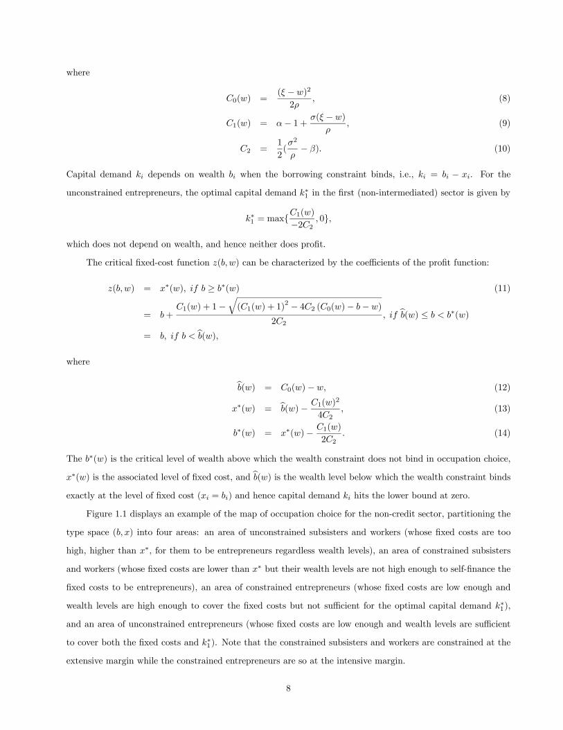
The critical fixed-cost function z(b, w) can be characterized by the coefficients of the profit function:
z(b,w) = x∗(w), if b ≥ b∗(w) (11)
= b+C1(w) + 1−
q(C1(w) + 1)
2 − 4C2 (C0(w)− b− w)
2C2, if bb(w) ≤ b < b∗(w)
= b, if b < bb(w),where
bb(w) = C0(w)− w, (12)
x∗(w) = bb(w)− C1(w)2
4C2, (13)
b∗(w) = x∗(w)− C1(w)
2C2. (14)
The b∗(w) is the critical level of wealth above which the wealth constraint does not bind in occupation choice,
x∗(w) is the associated level of fixed cost, and bb(w) is the wealth level below which the wealth constraint bindsexactly at the level of fixed cost (xi = bi) and hence capital demand ki hits the lower bound at zero.
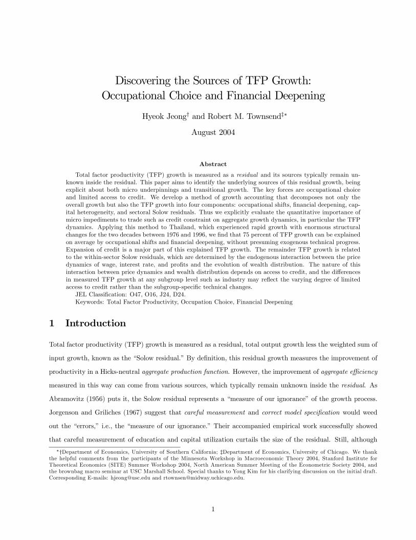
Figure 1.1 displays an example of the map of occupation choice for the non-credit sector, partitioning the
type space (b, x) into four areas: an area of unconstrained subsisters and workers (whose fixed costs are too
high, higher than x∗, for them to be entrepreneurs regardless wealth levels), an area of constrained subsisters
and workers (whose fixed costs are lower than x∗ but their wealth levels are not high enough to self-finance the
fixed costs to be entrepreneurs), an area of constrained entrepreneurs (whose fixed costs are low enough and
wealth levels are high enough to cover the fixed costs but not sufficient for the optimal capital demand k∗1),
and an area of unconstrained entrepreneurs (whose fixed costs are low enough and wealth levels are sufficient
to cover both the fixed costs and k∗1). Note that the constrained subsisters and workers are constrained at the
extensive margin while the constrained entrepreneurs are so at the intensive margin.
8

2.3 Credit Sector
Now suppose that there is a second sector with a credit market. Then, the borrowing constraint (4) is dropped,
and the cost of capital is an equilibrium interest rate r ≥ 1 that equates the supply and the demand for capitalin the credit market. The capital demand k∗2 of the second sector is given by
k∗2 = max{ρ(α− r) + σ(ξ − w)
ρβ − σ2, 0},
and the labor demand l∗2 by
l∗2 =ξ − w
ρ+
σ
ρk∗2 .
Every firm hires the same level of capital and labor of k∗2 and l∗2. Thus, unlike the first non-credit sector, firm
size does not vary over wealth in the credit sector, measured by either capital or labor. However, entrepreneurs
earn differential profits due to the differences in individual talent, i.e., the fixed cost xi.
Occupation choice in the credit sector is entirely determined by talent and not by individual wealth, where
the critical z∗(w, r) in credit sector is found by equating unconstrained profits with wage, i.e.,
z∗(w, r) = f(k∗2(w, r), l∗2(w, r))− wl∗2(w, r)− rk∗2(w, r)− w. (15)
An agent, whose xi is less than z∗(w, r), will establish a modern firm and earn optimal profits
π∗2(xi, w, r) = f(k∗2(w, r), l∗2(w, r))− wl∗2(w, r)− rk∗2(w, r)− xi. (16)
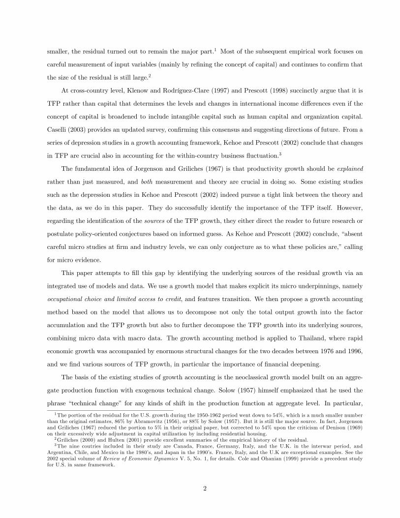
Figure 1.2 displays an example of the occupation choice map for the credit sector, partitioning the type space
(b, x) into two areas: an area of subsisters and workers and an area of entrepreneurs. Both groups are un-
constrained in their occupation choices. Entrepreneurs are again the agents who are more efficient in running
business and earn the rents to their talents in the form of profit. Hence, entrepreneurial income is always higher
than wage income. However, in the credit sector, neither distribution nor accumulation of wealth plays any
direct role in occupation choice. Occupation choice dynamics are determined only by the factor price dynamics
through z∗(w, r).
2.4 Financial Deepening
We combine the two sectors in one model with an exogenously expanding credit sector. By financial deepening,
what we have in mind is this expansion of access to credit on the extensive margin, rather than a within-credit-
sector deepening of intermediation level. Of course, the within-credit-sector deepening of intermediation is also
an important measure of financial deepening that may foster output growth. In fact, as we will see later, the role
of capital-deepening is important for the Thai output growth. However, we focus on the expansion of access to
credit on the extensive margin because it is a more direct channel of financial deepening to productivity growth.
9

Figure 2 displays several macro indicators of financial deepening such as total domestic credit, credit to
private sector, credit to public sector, and M3, all normalized by GDP, in Thailand.7 They suggests that the
financial sector has been continually deepened with a non-linear acceleration after the mid-1980’s. In particular,
the non-linear acceleration of financial deepening is more related to private credit rather than to M3, a broad
measure of liquid liabilities, or to public credit. Note that these macro indicators involve financial deepening on
both extensive and intensive margins. We count from the Socio-Economic Survey data, a nationally represen-
tative household survey in Thailand, the number of people who have actually used the financial institutions as
our measure of “financial deepening,” which better represents the expansion of access to credit on the extensive
margin.8 Figure 3 displays this measure of financial deepening, again showing a non-linear acceleration in the
middle of 1980’s. Both observations confirm that the feature of non-linear acceleration of financial deepening
is robust and is related to the our measure of financial deepening, i.e., the expansion of access to credit on the
extensive margin. This measure is embedded into the model as in the data.
The expansion of access to credit may well involve endogenous participation decisions as in Greenwood and
Jovanovic (1990). Here, we just exogenously impose the participation as in the data for the following reasons.
First, the exogeneity of financial deepening is in fact a reasonable assumption for our case. A large part of
financial sector expansion is would seems to be driven by exogenous financial sector reform and liberalization.
This is true in Thailand for the period of our analysis. See Alba, Hernandez, and Klingebiel (1999) for the
financial liberalization in Thailand.9
Second, Townsend and Ueda (2004) and Jeong and Townsend (2003) indeed bring the Greenwood and
Jovanovic (1990) model to the Thai data. Both papers simulate the financial participation choice at the estimated
Thai wealth distribution: the former paper at the calibrated parameter values fitting the growth dynamics at
aggregate level, while the latter paper at the estimated parameter values maximizing the likelihood of the
participation in the financial sector at micro level. Neither of them could endogenously generate the non-linear
acceleration of financial deepening in Thailand, shown in Figure 2. Thus, these previous studies suggest that
a big part of the Thai financial deepening seems to be determined by some exogenous forces, in particular the
non-linear acceleration in the middle 1980’s, which will play a key role in identifying the sources of TFP growth
in Thailand.7The Bank of Thailand provides raw data for these indicators.8 See Data Appendix for details of calculating this measure of financial deepening from the SES data.9Noticeable financial reform policies in Thailand initiated around the critical year 1986 include: 1) liberalization of current
and capital account; 2) removal of interest rate controls (preferential lending rates to priority sectors, ceiling rates on depositand lending); 3) expanding the scope of activities of commercial banks and finance companies (provision of custodial services,information service, financial consulting service, loan syndication, sales of government bonds, relaxation of requirement of portfoliocomposition, for example, on the minimum required credit to agricultural sector). Another important event that would contributeto expanding the extent of the financial sector is a creation of deposit insurance program, Financial Institutions Development Fund(FIDF) in 1985, a legal entity under the Bank of Thailand that mandates to provide liquidity support to financial institutions. TheFIDF was a response to the financial crisis during the period 1983-1987.
10
Third, we intentionally shut down all exogenous technological changes, the typical engine of productivity
growth in the existing TFP literature. Thus, in our model, productivity growth does not come from technical
changes but from improving allocation efficiency, which depends on financial deepening. This is not because
we think technical change is unimportant, but rather we would like to see how well the alternative hypothesis
of growth based on occupational choice and financial deepening can explain the actual growth of output and
TFP. By assuming the financial deepening to be exogenous, we hope to take a fair footing with the typical TFP
literature, where the main engine of growth, i.e., technical changes, is assumed to be exogenous.
2.5 Sources of Productivity Growth
In this model, households of varying talent face an imperfect credit market in financing the establishment of
business and in expanding the scale of enterprise. Thus, households are constrained by limited wealth on an
extensive margin of occupation choice and an intensive margin of capital demand, though both constraints
can be alleviated over time as wealth accumulates. Occupational choices determine the differential levels of
productivity of the commonly-given one unit of time of the agents, due to the income gaps across occupations.
Thus, pure occupational shift at given level of financial deepening can be a source of productivity growth.
Financial deepening relaxes borrowing constraints both on the extensive and intensive margins and enhances
the productivity of the economy. Thus, as the distribution of wealth evolves and financial sector deepens, so
does the occupational composition of population and the allocation efficiency of capital and labor, generating
the dynamics of aggregate output and productivity growth.
Limited access to credit and the existence of fixed-cost capital create heterogeneity in capital since the
non-intermediated capital and the fixed-cost capital earns zero net return. Note that this kind of heterogeneity
is not about adjusting the quality variation in capital. It is hard to capture this effect using the standard
aggregate production function.10 This is in fact a matter of measurement, not productivity growth. However,
in the standard growth accounting framework, this is can be inside the residual measure of TFP growth.
There are some noticeable implications in this dynamics of productivity growth along with the evolution of
wealth and financial deepening. First, the expansion of access to credit does not necessarily promote entrepre-
neurship. Among poor people, having access to credit helps them to relax the constraint at the extensive margin
and it encourages the poor but talented people to become entrepreneurs. Hence the fraction of entrepreneurs is
larger in the credit sector than in the non-credit sector. Compare the two occupation maps Figure 1.1 and 1.2 at
the wealth levels lower than bb, for example. Among rich people, however, who rarely face borrowing constraints,10The problem from the usual capital homogeneity assumption in aggregate production function approach was noticed early by
Hicks (1965) and again cogently stated by Schultz (1988), “the simplifying assumption that capital is homogeneous is a disasterto capital theory (Hicks, 1965), and ... is subject to serious doubts. · · · The dynamics of economic growth is afloat on capitalinequalities because of the differences in rates of returns when disequilibria prevail, · · · Thus, one of the essential parts of economicgrowth is concealed by such aggregation.”
11

the incentive to become entrepreneurs is less in the credit sector than in the non-credit sector because people
in the credit sector can deposit their wealth in the banks and earn positive net return while the agents in the
non-credit sector cannot. Again compare Figures 1.1 and 1.2 at the wealth levels exceeding b∗. It is easy to
show that the critical level that determines the extensive margin of unconstrained subsisters and workers is
always lower in the credit sector than in the non-credit sector, i.e.,
z∗(w, r) ≤ x∗(w), for each w and r ≥ 1,
and the gap x∗(w)− z∗(w, r) increases in r for every given wage w so that .11 Thus, the expansion of access to
credit may promote or diminish entrepreneurship. It depends on wealth distribution.
Second, recall that the model implies a take-off feature of wage dynamics, i.e., wage eventually picks up as
the labor demand increases along with growth. Both credit and non-credit sectors face the same wage growth
but the response to this common wage growth is asymmetric between the two sectors. Within the non-credit
sector, wage growth helps wealth accumulation of the talented but poor wageworkers, and possibly (depending
on the magnitude of the wage growth) encourages them to switch their occupation into entrepreneurs, and
hence improve the productivity growth. In the credit sector, the occupational choices are already efficient and
occupational shifts depend only on the movement of factor prices. In fact, an increase in the wage reduces the
fraction of entrepreneurs as well as the profits in the credit sector since z∗(w, r) and optimal profit function
π∗2(xi, w, r) are decreasing function in wage w in credit sector from the Envelope theorem. That is, for the
credit sector, wage growth discourages entrepreneurship. Thus, there are counteracting effects of wage growth
on overall productivity growth.
Third, the average firm size increases with financial deepening. This is obvious since the scale of enterprise
is always smaller in the non-credit sector due to the wealth constraints than in the credit sector. As we already
discussed, financial deepening enhances productivity growth as well. Thus, we may observe a growth in firm size
accompanied by productivity growth. But both kinds of growth come from financial deepening as a common
fundamental source.11First, note that the wage w is common to both sectors and the difference regarding the critical values of setup cost between
the two sectors comes from the interest rate r, i.e., r ≥ 1 for credit sector but the interest rate for non-credit sector is set to unity.Second, it is easy to check that z∗(w, r) = x∗(w) when r = 1. Thus, it is enough to show that z∗(w, r) is a monotonically decreasingin r, which is as follows:
∂z∗(w, r)∂r
= fk(k∗2 , l∗2)∂k∗2(w, r)
∂r+ fl(k
∗2 , l∗2)∂l∗2(w, r)
∂r−w
∂l∗2(w, r)∂r
− k∗2(w, r)− r∂k∗2(w, r)
∂r
= [fk(k∗2 , l∗2)− r]
∂k∗2(w, r)∂r
+ [fl(k∗2 , l∗2)− r]
∂l∗2(w, r)∂r
− k∗2(w, r)
= −k∗2(w, r) ≤ 0.The second equality comes from the first-order conditions of profit maximization in the credit sector.
12

3 Method of Growth Accounting
The self-selection feature, constrained or unconstrained occupation choice, yields non-zero profits and makes the
typical constant-returns-to-scale framework of growth accounting (presuming zero profits) inapplicable, either
the primary or dual versions. In particular, the financial-deepening effect on productivity growth emerges from
the constrained choice on both extensive margin (occupation choice) and intensive margin (scale of firms), hence
the differential profitability between the credit and non-credit sectors. Also imposing constant-returns-to-scale
precludes the differential interaction between profits and wage depending on the access to credit, and hence
the results of typical dual growth accounting using only factor prices with ignoring profits may be misleading
as well. Here, we develop a method of growth accounting that is adapted to the above growth model with
occupational choices under limited access to credit.
3.1 Aggregation of Two-Sector Economy
There are two sectors, one without access to credit (sector 1) and the other with access to credit (sector 2). The
three occupations are self-employed subsisters using traditional technology, wageworkers, and entrepreneurs
using modern technology. The labor market is integrated and wage rate w is common between two sectors.
However, the capital market is exogenously segmented, where the opportunity cost of capital differs between
the two sectors: it is unity, tied to the backyard storage technology, in sector 1, but it is the equilibrium interest
rate r of the credit market in sector 2. Owing to the exogenously embedded segmentation, we can derive the
aggregate relationships within each sector separately and then add them up to get economy-wide aggregate
relationship.
3.1.1 Aggregation Within Sectors
Given equilibrium wage rate w, the profit πi1 of an agent i with fixed cost xi and wealth bi who chooses to be
an entrepreneur (or a modern firm) in sector 1 is given by:
πi1 = π1(bi, xi, w)
= f(li1, ki1)− wli1 − ki1 − xi, (17)
where li1 and ki1 denote optimal demands for labor and capital, respectively:
li1 = l1(bi, xi, w),
ki1 = k1(bi, xi, w).
13

Thus, the output ymi1 of the modern firm i in sector 1 by simply rearranging (17) can be expressed:
ymi1 = f(li1, ki1)
= π1(bi, xi, w) + wl1(bi, xi, w) + k1(bi, xi, w) + xi,
and the total output Y m1 of all modern firms in sector 1 is given by:
Y m1 = Π1 + wLm1 +Km
1 +X1, (18)
defining
Π1 =
Z ∞0
Z z(b,w)
0
π1(b, x,w)dH(x)dΨ1(b),
Lm1 =
Z ∞0
Z z(b,w)
0
l1(b, x,w)dH(x)dΨ1(b),
Km1 =
Z ∞0
Z z(b,w)
0
k1(b, x,w)dH(x)dΨ1(b),
X1 =
Z z(b,w)
0
xdH(x),
where z(b, w) is given in (11), Ψ1 denotes cumulative distribution function of wealth in sector 1 (which endoge-
nously evolves over time), and H the time-invariant distribution function of fixed cost. Equation (18) indicates
that the output produced in sector 1 is decomposed into profits Π1, wage payment wLm1 , contribution of working
capital Km1 , and the contribution of fixed-cost capital X1. Note that depreciation of capital is not incorporated
in this model. Also note the explicit inclusion of fixed cost, which is not typical in standard income accounting.
The population in sector 1 is partitioned into three occupations, the fractions of which are given:
Φe1 =
Z ∞0
Z z(b,w)
0
dH(x)dΨ1(b) for entrepreneurs,
Φw1 = Lm1 for wage laborers,
Φs1 = 1− Φe1 − Φw1 for traditional subsisters.
Thus, total output from traditional technology in sector 1 is
Y s1 = Φ
s1γ. (19)
Let K1 denote the total wealth in sector 1. Wealth that is not used for modern production, K1 −Km1 −X1 is
invested in the backyard storage technology and produces output Y b1 with the rate of return of unity:
Y b1 = K1 −Km
1 −X1. (20)
Combining these three sources of output production in (18), (19), and (20), we get the total output in
14

sector 1, Y1:
Y1 = Y m1 + Y s
1 + Y b1
= Π1 + wLm1 +Km1 +X1 +Φ
s1γ +K1 −Km
1 −X1
= Π1 + wΦw1 +Φs1γ +K1.
When both traditional and modern technologies coexist, the wage is set to reservation wage at w = γ, and hence
wΦw1 +Φs1γ = wL1, where L1 ≡ 1−Φe1. Note that L1 indicates the population proportion of non-entrepreneurs
in sector 1. When the surplus labor is exhausted and wage endogenously starts to grow exceeding γ, Φs1 = 0,
and again wΦw1 +Φs1γ = wL1. Therefore, total output in sector 1 can be written as
Y1 = Π1 + wL1 +K1. (21)
Note that here the size of population in sector 1 is normalized to one. Equation (21) states simply that output
per capita in sector 1 is the sum of factor payments (profit, wage income, and rental income) with the rental
rate of capital being set to unity.
In sector 2, where the credit market is open, the profit πi2 of an agent i with fixed cost xi and wealth bi
who chooses to be a modern firm in sector 2 is given by:
πi2 = π2(xi, w, r)
= f(li2, ki2)− wli2 − rki2 − xi,
where li2 and ki2 denote unconstrained demands for labor and capital that depend only on market factor prices,
i.e.,
li2 = l2(w, r),
ki2 = k2(w, r).
Note that entrepreneurial talent, i.e., fixed cost has an influence in this model only on the extensive margin
of occupation choice, not the intensive margin of factor demands. This again implies that the size of modern
firm is identical across firms in the intermediated credit sector, although they may earn different levels of profit,
depending on innate entrepreneurial talent xi.
Total output from all modern firms in sector 2 Y m2 can be similarly derived:
Y m2 = Π2 + wLm2 + rKm
2 +X2, (22)
15
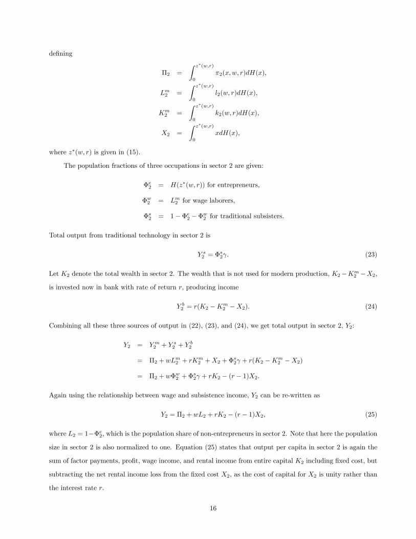
defining
Π2 =
Z z∗(w,r)
0
π2(x,w, r)dH(x),
Lm2 =
Z z∗(w,r)
0
l2(w, r)dH(x),
Km2 =
Z z∗(w,r)
0
k2(w, r)dH(x),
X2 =
Z z∗(w,r)
0
xdH(x),
where z∗(w, r) is given in (15).
The population fractions of three occupations in sector 2 are given:
Φe2 = H(z∗(w, r)) for entrepreneurs,
Φw2 = Lm2 for wage laborers,
Φs2 = 1− Φe2 − Φw2 for traditional subsisters.
Total output from traditional technology in sector 2 is
Y s2 = Φ
s2γ. (23)
Let K2 denote the total wealth in sector 2. The wealth that is not used for modern production, K2−Km2 −X2,
is invested now in bank with rate of return r, producing income
Y b2 = r(K2 −Km
2 −X2). (24)
Combining all these three sources of output in (22), (23), and (24), we get total output in sector 2, Y2:
Y2 = Y m2 + Y s
2 + Y b2
= Π2 + wLm2 + rKm2 +X2 +Φ
s2γ + r(K2 −Km
2 −X2)
= Π2 + wΦw2 +Φs2γ + rK2 − (r − 1)X2.
Again using the relationship between wage and subsistence income, Y2 can be re-written as
Y2 = Π2 + wL2 + rK2 − (r − 1)X2, (25)
where L2 = 1−Φe2, which is the population share of non-entrepreneurs in sector 2. Note that here the populationsize in sector 2 is also normalized to one. Equation (25) states that output per capita in sector 2 is again the
sum of factor payments, profit, wage income, and rental income from entire capital K2 including fixed cost, but
subtracting the net rental income loss from the fixed cost X2, as the cost of capital for X2 is unity rather than
the interest rate r.
16

3.1.2 Aggregation Between Sectors
Let p be the fraction of the intermediated sector in the entire economy. Then, economy-wide per capita output
Y is a weighted sum of sectoral outputs Y1 and Y2:
Y = (1− p)Y1 + pY2. (26)
National income accounting suggests that the output Y can be decomposed into factor payments such that
Y = wL+ rK − (r − 1)U +Π. (27)
Thus, there are two ways of expressing the level of output Y , one decomposed by sector as in (26), and the other
decomposed by factor as in (27). It is easy to check they yield the same output from the following identities:
L = (1− p)L1 + pL2, (28)
K = (1− p)K1 + pK2, (29)
U = (1− p)K1 + pX2, (30)
Π = (1− p)Π1 + pΠ2. (31)
There are two differences in our national-income-accounting identity in equation (27) from the standard one.
First, profit income Π is explicitly included. If the underlying technology were subject to constant returns to
scale and the aggregate capital K captured all relevant capital factors, Π would be zero. Second, there is an
adjustment term −(r− 1)U , where U is a weighted sum of total capital in no-credit sector, K1, and the capital
used for fixed cost in credit sector, X2. These two kinds of capital do not earn positive net returns. In the
income accounting equation (27), the aggregate capital of the whole economy K is priced by the gross interest
rate r. The adjustment term corrects this mis-measurement of capital income, first due to the limited access to
credit market, and second due to the existence of the presumed fixed cost.
3.2 Decomposition of TFP Growth
In this model, the aggregate TFP growth does not remain as a residual but can be further decomposed into
its underlying sources. Main idea is that growth accounting by factor and growth accounting by sector should
each yield the same output growth. By equating the two versions of growth accounting, we can identify the
sources of aggregate TFP growth in terms of the sectoral TFP growth and the various compositional changes
on the extensive margins such as occupational shifts and expansion of credit sector (our measure of financial
deepening).
17

3.2.1 Growth Accounting by Factor
By differentiating both sides of (27) with respect to time and then dividing them by total output in base year,
we get a growth accounting identity by factor:
gY = sL(gL + gw) + sK(gK + gr)− sU (gU +
µr
r − 1¶gr) + sΠgΠ, (32)
where
sL =wL
Y, sK =
rK
Y, sU =
(r − 1)UY
, sΠ =Π
Y, (33)
and gV denotes the growth rate of variable V .12 This simply tells that the output growth is decomposed into
growth in input quantities and growth in input prices, each being weighted by appropriate factor share. Then,
the TFP growth TFPG can be measured by subtracting the growth in weighted sum of input quantities from
the output growth such that:
TFPG ≡ gY − (sKgK − sUgU )− sLgL. (34)
This is the familiar primary measure of TFP growth. The accounting identity (32) implies that the same TFP
growth can be measured in dual version in terms of price growth of inputs:13
TFPG = sLgw +
·sK − sU
µr
r − 1¶¸
gr + sΠgΠ. (35)
Note that both versions of TFP growth measure incorporate two kinds of heterogeneity, heterogeneous labor
and capital. The same unit of time endowment is devoted to different kinds of income-generating activities across
different occupations, which generates a heterogeneity for labor. Laborers and traditional subsisters earn less
income than entrepreneurs doing different kinds of income-generation activities. Thus, aggregate productivity is
enhanced as the population share of laborers and traditional subsisters, L, decreases. The term −sLgL capturesthis effect of occupational shift.
The existence of the fixed cost and limited access to credit market generate the heterogeneity in capital
via differential costs of capital between the working capital and the fixed-cost capital, and also between the
intermediated and non-intermediated sectors. The variable U in equation (30) measures the capital, the net
12The growth accounting formula in (32) is written as a growth rate of Divisia index in continuous time. In practice, withdiscrete-time data, we use the following decomposition formula between initial period s and final period t :
gY =wΦs
YsgΦ +
wsΦ
Ysgw +
rKs
YsgK +
rsK
Ysgr
− (r − 1)UsYs
gU +(rs − 1)U
Ysgr +
Πs
YsgΠ,
where the upper bar denotes the average between periods s and t. Note that this formula is similar to the Tornqvist approximation(that uses average of factor shares between dates) to the Divisia index, but our formula for discrete data is an exact decompositionrather than an approximation. Hereafter, we apply this decomposition formula to all the following growth accounting identities.13Hsieh (2002) provides a clear discussion on the use of the dual framework in accounting for the East Asian economic growth,
but he does not put much emphasis on the profit component and the capital-heterogeneity effect in his application. We will seelater that profit plays a key role in explaining the TFP growth in various ways.
18
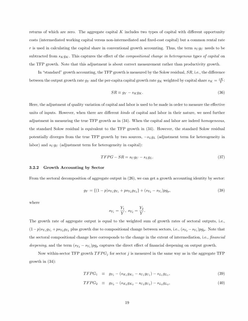
returns of which are zero. The aggregate capital K includes two types of capital with different opportunity
costs (intermediated working capital versus non-intermediated and fixed-cost capital) but a common rental rate
r is used in calculating the capital share in conventional growth accounting. Thus, the term sUgU needs to be
subtracted from sKgK . This captures the effect of the compositional change in heterogenous types of capital on
the TFP growth. Note that this adjustment is about correct measurement rather than productivity growth.
In “standard” growth accounting, the TFP growth is measured by the Solow residual, SR, i.e., the difference
between the output growth rate gY and the per-capita capital growth rate gK weighted by capital share sK = rKY :
SR ≡ gY − sKgK . (36)
Here, the adjustment of quality variation of capital and labor is used to be made in order to measure the effective
units of inputs. However, when there are different kinds of capital and labor in their nature, we need further
adjustment in measuring the true TFP growth as in (34). When the capital and labor are indeed homogeneous,
the standard Solow residual is equivalent to the TFP growth in (34). However, the standard Solow residual
potentially diverges from the true TFP growth by two sources, −sLgL (adjustment term for heterogeneity in
labor) and sUgU (adjustment term for heterogeneity in capital):
TFPG− SR = sUgU − sLgL. (37)
3.2.2 Growth Accounting by Sector
From the sectoral decomposition of aggregate output in (26), we can get a growth accounting identity by sector:
gY = {(1− p)sY1gY1 + psY2gY2}+ (sY2 − sY1)pgp, (38)
where
sY1 =Y1Y, sY2 =
Y2Y.
The growth rate of aggregate output is equal to the weighted sum of growth rates of sectoral outputs, i.e.,
(1−p)sY1gY1 +psY2gY2 plus growth due to compositional change between sectors, i.e., (sY2 −sY1)pgp. Note thatthe sectoral compositional change here corresponds to the change in the extent of intermediation, i.e., financial
deepening, and the term (sY2 − sY1)pgp captures the direct effect of financial deepening on output growth.
Now within-sector TFP growth TFPGj for sector j is measured in the same way as in the aggregate TFP
growth in (34):
TFPG1 ≡ gY1 − (sK1gK1 − sU1gU1)− sL1gL1 , (39)
TFPG2 ≡ gY2 − (sK2gK2 − sU2gU2)− sL2gL2 , (40)
19

where U1 = K1 and U2 = X2, and
sL1 =wL1Y1
, sK1 =rK1
Y1, sU1 =
(r − 1)K1
Y1, sL2 =
wL2Y2
, sK2 =rK2
Y2, and sU2 =
(r − 1)X2
Y2.
That is, the within-sector growth rates gY1 and gY2 can be expressed:
gY1 = TFPG1 + (sL1gL1 + sK1gK1− sU1gU1), (41)
gY2 = TFPG2 + (sL2gL2 + sK2gK2 − sU2gU2), (42)
Substituting these within-sector growth rates in (41) and (42) into the growth accounting identity by sector in
(38), we get
gY = (sY2 − sY1)pgp + (1− p)sY1TFPG1 + psY2TFPG2 (43)
+(1− p)sY1(sL1gL1 + sK1gK1 − sU1gK1) + psY2(sL2gL2 + sK2gK2 − sU2gX2).
From the formula for the aggregate TFP growth in (34), we have the following identity:
gY = TFPG+ sLgL + sKgK − sUgU . (44)
Now decompose the aggregate growth of each factor (gL, gK , and gU ) in (44) into sectoral factor growth:
gL =gsL1(1− p)gL1 +gsL2pgL2 + (gsL2 −gsL1)pgp, (45)
gK =gsK1(1− p)gK1
+gsK2pgK2
+ (gsK2−gsK1
)pgp, (46)
gU =gsU1(1− p)gU1 +gsU2pgU2 + (gsU2 −gsU1)pgp, (47)
where
gsL1 = L1L, gsL2 = L2
L, gsK1 =
K1
K, gsK2 =
K2
K, gsU1 = K1
U, andgsU2 = X2
U.
Substituting the equations (45) to (47) into the aggregate factor growth in (44), we get
gY = TFPG+ [sY2(sL2 + sK2 − sU2)− sY1(sL1 + sK1 − sU1)]pgp + (48)
(1− p)sY1(sL1gL1 + sK1gK1 − sU1gK1) + psY2(sL2gL2 + sK2gK2 − sU2gX2).
Equating the two versions of growth accounting identity (43) and (48), the aggregate TFP growth is decomposed
such that:
TFPG = (1− p)sY1TFPG1 + psY2TFPG2 (49)
+(sY2 − sY1)pgp − [sY2(sL2 + sK2 − sX2)− sY1(sL1 + sK1)]pgp.
20
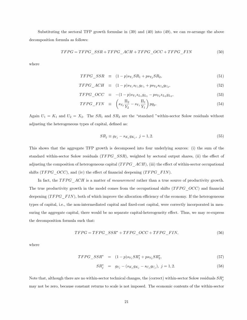
Substituting the sectoral TFP growth formulae in (39) and (40) into (49), we can re-arrange the above
decomposition formula as follows:
TFPG = TFPG_SSR+ TFPG_ACH + TFPG_OCC + TFPG_FIN (50)
where
TFPG_SSR ≡ (1− p)sY1SR1 + psY2SR2, (51)
TFPG_ACH ≡ (1− p)sY1sU1gU1 + psY2sU2gU2 , (52)
TFPG_OCC ≡ −(1− p)sY1sL1gL1 − psY2sL2gL2 , (53)
TFPG_FIN ≡µsY2Π2Y2− sY1
Π1Y1
¶pgp. (54)
Again U1 = K1 and U2 = X2. The SR1 and SR2 are the “standard ”within-sector Solow residuals without
adjusting the heterogeneous types of capital, defined as:
SRj ≡ gYj − sKjgKj , j = 1, 2. (55)
This shows that the aggregate TFP growth is decomposed into four underlying sources: (i) the sum of the
standard within-sector Solow residuals (TFPG_SSR), weighted by sectoral output shares, (ii) the effect of
adjusting the composition of heterogeneous capital (TFPG_ACH), (iii) the effect of within-sector occupational
shifts (TFPG_OCC), and (iv) the effect of financial deepening (TFPG_FIN).
In fact, the TFPG_ACH is a matter of measurement rather than a true source of productivity growth.
The true productivity growth in the model comes from the occupational shifts (TFPG_OCC) and financial
deepening (TFPG_FIN), both of which improve the allocation efficiency of the economy. If the heterogeneous
types of capital, i.e., the non-intermediated capital and fixed-cost capital, were correctly incorporated in mea-
suring the aggregate capital, there would be no separate capital-heterogeneity effect. Thus, we may re-express
the decomposition formula such that:
TFPG = TFPG_SSR∗ + TFPG_OCC + TFPG_FIN, (56)
where
TFPG_SSR∗ = (1− p)sY1SR∗1 + psY2SR
∗2, (57)
SR∗j = gYj − (sKjgKj − sUjgUj ), j = 1, 2. (58)
Note that, although there are no within-sector technical changes, the (correct) within-sector Solow residuals SR∗j
may not be zero, because constant returns to scale is not imposed. The economic contents of the within-sector
21
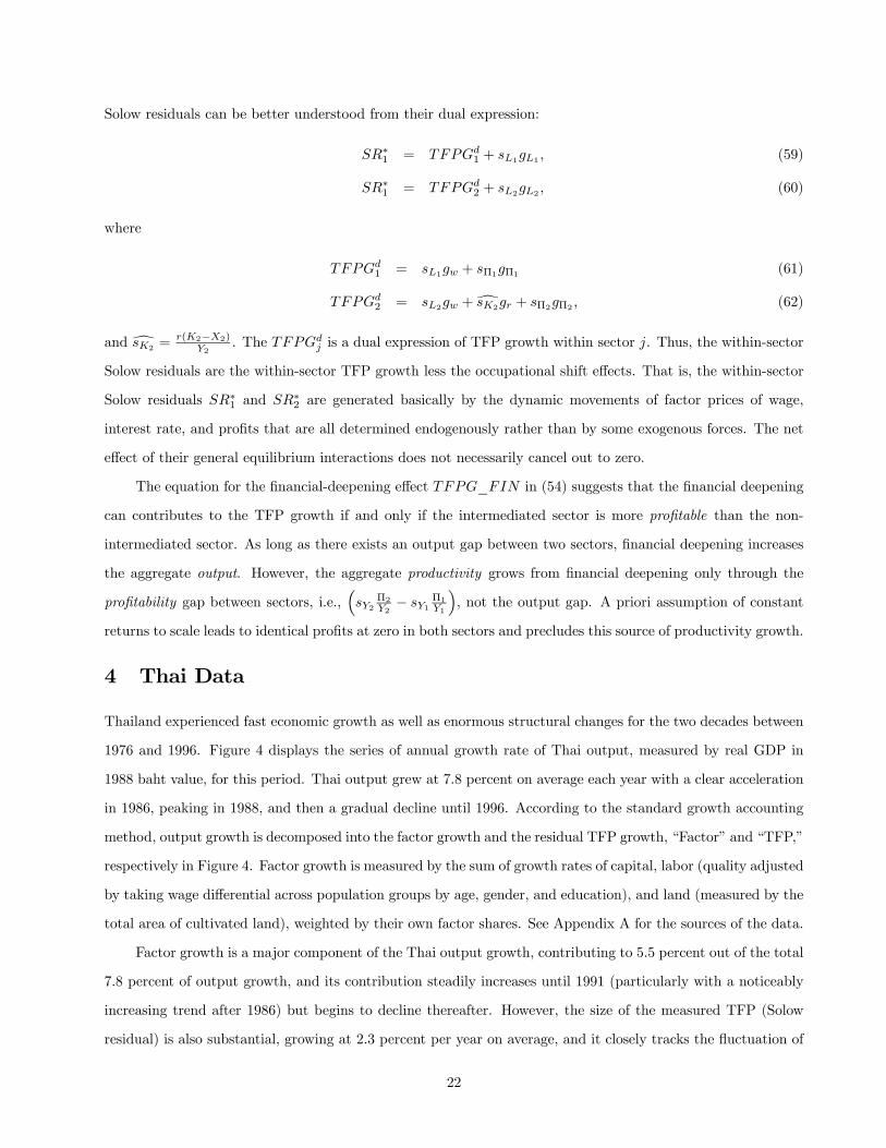
Solow residuals can be better understood from their dual expression:
SR∗1 = TFPGd1 + sL1gL1 , (59)
SR∗1 = TFPGd2 + sL2gL2 , (60)
where
TFPGd1 = sL1gw + sΠ1gΠ1 (61)
TFPGd2 = sL2gw +dsK2gr + sΠ2gΠ2 , (62)
and dsK2 =r(K2−X2)
Y2. The TFPGd
j is a dual expression of TFP growth within sector j. Thus, the within-sector
Solow residuals are the within-sector TFP growth less the occupational shift effects. That is, the within-sector
Solow residuals SR∗1 and SR∗2 are generated basically by the dynamic movements of factor prices of wage,
interest rate, and profits that are all determined endogenously rather than by some exogenous forces. The net
effect of their general equilibrium interactions does not necessarily cancel out to zero.
The equation for the financial-deepening effect TFPG_FIN in (54) suggests that the financial deepening
can contributes to the TFP growth if and only if the intermediated sector is more profitable than the non-
intermediated sector. As long as there exists an output gap between two sectors, financial deepening increases
the aggregate output. However, the aggregate productivity grows from financial deepening only through the
profitability gap between sectors, i.e.,³sY2
Π2Y2− sY1
Π1Y1
´, not the output gap. A priori assumption of constant
returns to scale leads to identical profits at zero in both sectors and precludes this source of productivity growth.
4 Thai Data
Thailand experienced fast economic growth as well as enormous structural changes for the two decades between
1976 and 1996. Figure 4 displays the series of annual growth rate of Thai output, measured by real GDP in
1988 baht value, for this period. Thai output grew at 7.8 percent on average each year with a clear acceleration
in 1986, peaking in 1988, and then a gradual decline until 1996. According to the standard growth accounting
method, output growth is decomposed into the factor growth and the residual TFP growth, “Factor” and “TFP,”
respectively in Figure 4. Factor growth is measured by the sum of growth rates of capital, labor (quality adjusted
by taking wage differential across population groups by age, gender, and education), and land (measured by the
total area of cultivated land), weighted by their own factor shares. See Appendix A for the sources of the data.
Factor growth is a major component of the Thai output growth, contributing to 5.5 percent out of the total
7.8 percent of output growth, and its contribution steadily increases until 1991 (particularly with a noticeably
increasing trend after 1986) but begins to decline thereafter. However, the size of the measured TFP (Solow
residual) is also substantial, growing at 2.3 percent per year on average, and it closely tracks the fluctuation of
22
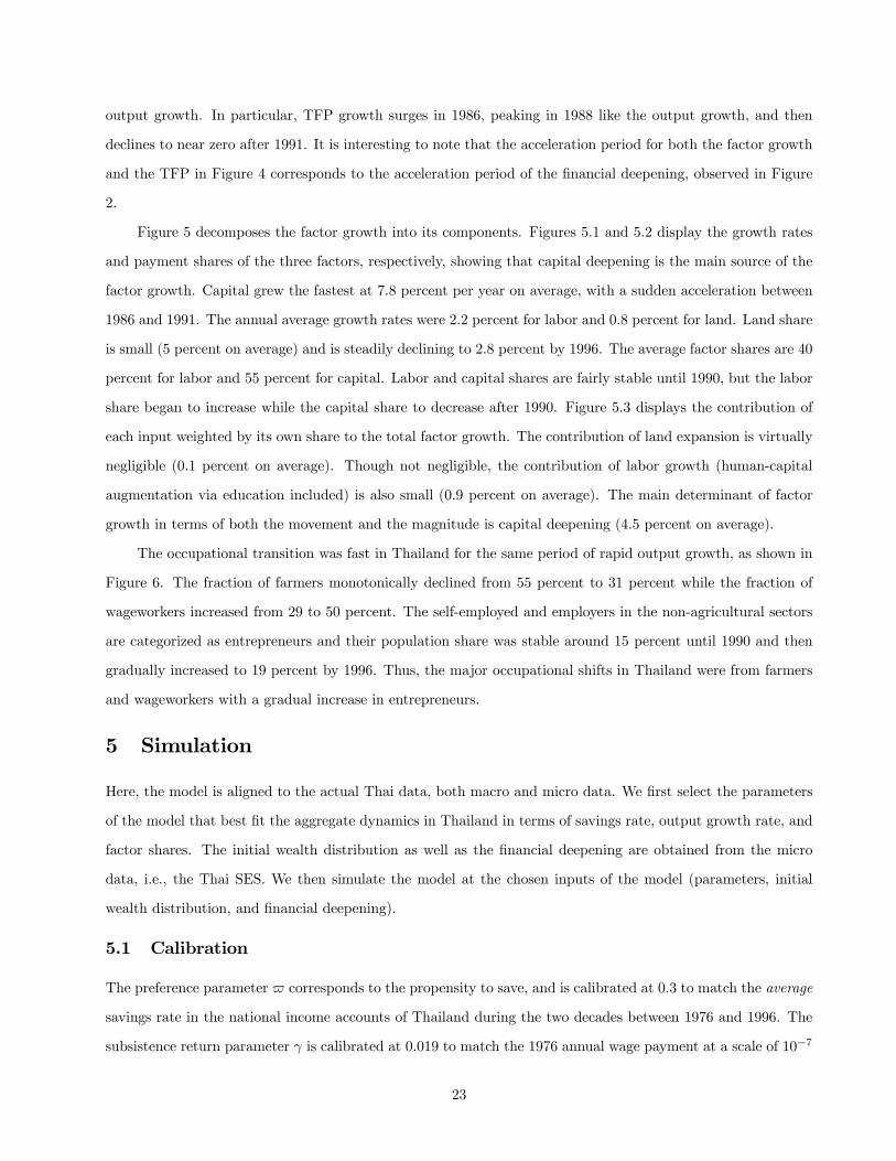
output growth. In particular, TFP growth surges in 1986, peaking in 1988 like the output growth, and then
declines to near zero after 1991. It is interesting to note that the acceleration period for both the factor growth
and the TFP in Figure 4 corresponds to the acceleration period of the financial deepening, observed in Figure
2.
Figure 5 decomposes the factor growth into its components. Figures 5.1 and 5.2 display the growth rates
and payment shares of the three factors, respectively, showing that capital deepening is the main source of the
factor growth. Capital grew the fastest at 7.8 percent per year on average, with a sudden acceleration between
1986 and 1991. The annual average growth rates were 2.2 percent for labor and 0.8 percent for land. Land share
is small (5 percent on average) and is steadily declining to 2.8 percent by 1996. The average factor shares are 40
percent for labor and 55 percent for capital. Labor and capital shares are fairly stable until 1990, but the labor
share began to increase while the capital share to decrease after 1990. Figure 5.3 displays the contribution of
each input weighted by its own share to the total factor growth. The contribution of land expansion is virtually
negligible (0.1 percent on average). Though not negligible, the contribution of labor growth (human-capital
augmentation via education included) is also small (0.9 percent on average). The main determinant of factor
growth in terms of both the movement and the magnitude is capital deepening (4.5 percent on average).
The occupational transition was fast in Thailand for the same period of rapid output growth, as shown in
Figure 6. The fraction of farmers monotonically declined from 55 percent to 31 percent while the fraction of
wageworkers increased from 29 to 50 percent. The self-employed and employers in the non-agricultural sectors
are categorized as entrepreneurs and their population share was stable around 15 percent until 1990 and then
gradually increased to 19 percent by 1996. Thus, the major occupational shifts in Thailand were from farmers
and wageworkers with a gradual increase in entrepreneurs.
5 Simulation
Here, the model is aligned to the actual Thai data, both macro and micro data. We first select the parameters
of the model that best fit the aggregate dynamics in Thailand in terms of savings rate, output growth rate, and
factor shares. The initial wealth distribution as well as the financial deepening are obtained from the micro
data, i.e., the Thai SES. We then simulate the model at the chosen inputs of the model (parameters, initial
wealth distribution, and financial deepening).
5.1 Calibration
The preference parameter corresponds to the propensity to save, and is calibrated at 0.3 to match the average
savings rate in the national income accounts of Thailand during the two decades between 1976 and 1996. The
subsistence return parameter γ is calibrated at 0.019 to match the 1976 annual wage payment at a scale of 10−7
23

that converts Thai baht unit into the model income unit. Here, we suppose the 1976 Thai wage to be close to
the reservation wage, and hence the subsistence income (w = γ) in the model. In fact, the occupational shift
from farmers to wage earners was fast in the Thai economy during the first decade of 1976-1986. The fraction
of farmers went down from 55% to 46% while the fraction of wageworkers increased from 29% to 38%. (See
Figure 6.) But the Thai wage stayed constant during this period. According to the model, the compositional
change between wageworkers and subsisters with constant wage can only happen at the reservation wage. Thus
the approximation of γ by the 1976 wage seems reasonable.
To be consistent, the Thai initial wealth distribution is put into the model using the same scale. Given
the bounded support and additive nature of the fixed cost x and the borrowing constraint in (4), the choice of
scale is important for the growth dynamics of the model, not only through the value of γ but also through the
scale of initial wealth distribution.14
Conditional on , γ, and scale parameter, the technology parameters α, β, ξ, ρ, and σ are calibrated to
match the key aggregate objects in growth accounting exercise, i.e., the paths of GDP growth rate and labor
share in Thailand for the period of 1976-1996, using an explicit root-mean-squared-error (RMSE) criterion (the
two variables being equally weighted). Thus the model economy is aligned to mimic the patterns of aggregate
growth of the actual Thai economy. Table 1 summarizes the selected parameters.
Table 1. Model Parametersγ α β ξ ρ σ
0.30 0.019 1.111 0.001 0.100 0.0063 0.000
5.2 Aggregate Dynamics
The simulated economy tracks output growth and the labor share of Thailand well, as is shown in Figures 7.1
and 7.2. The simulated annual growth rate is a little lower than the actual Thai data (varying from 4 to 14
percent), which may indicate that the model misses some engines of growth in Thailand. However, the dynamic
patterns of the Thai growth, the slow-down in early 1980’s, the surge after 1986, and the continual decline
thereafter, are very well captured by the model. The simulated labor share is a little lower than the Thai data
(varying from 35 to 45 percent), but again the model captures dynamic patterns such as the upturn of the
labor share after 1990 in the data. The upturn is mainly due to the wage growth rather than the change in
employment, both in the model and the data.
14For instance, the higher the scale is, i.e., the wealthier the model economy becomes, the higher is the fraction of entrepreneurs,but too much wealth can induce the agents to consume their wealth rather than save it and the economy suffers from negativegrowth initially. The higher is the scale, the greater is the tendency toward the initial negative growth, although this relationship isnot monotone. Eventually the economy starts to grow, but overall growth for the entire sampling period can be negative when theinitial negative growth is too large. From our previous study in Jeong and Townsend (2003), we know the range of scale parameterwhere the simulated aggregate output growth is positive at the given Thai initial wealth distribution, and we restrict the search ofscale within this range.
24
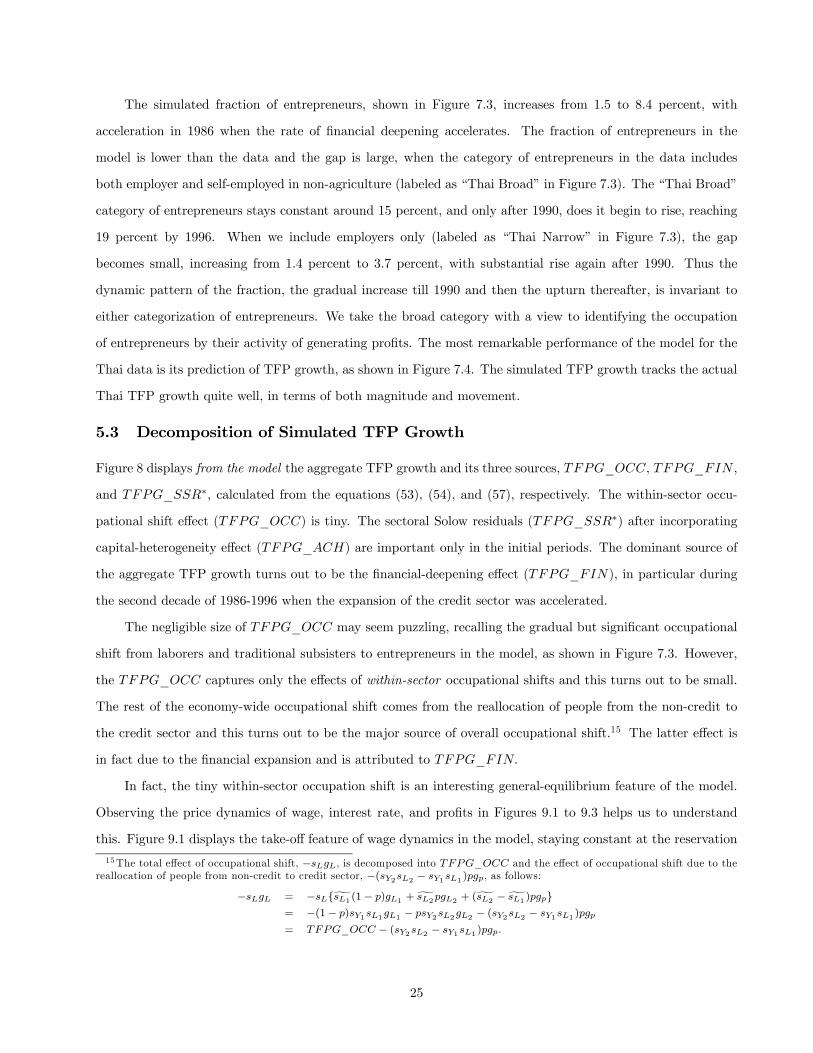
The simulated fraction of entrepreneurs, shown in Figure 7.3, increases from 1.5 to 8.4 percent, with
acceleration in 1986 when the rate of financial deepening accelerates. The fraction of entrepreneurs in the
model is lower than the data and the gap is large, when the category of entrepreneurs in the data includes
both employer and self-employed in non-agriculture (labeled as “Thai Broad” in Figure 7.3). The “Thai Broad”
category of entrepreneurs stays constant around 15 percent, and only after 1990, does it begin to rise, reaching
19 percent by 1996. When we include employers only (labeled as “Thai Narrow” in Figure 7.3), the gap
becomes small, increasing from 1.4 percent to 3.7 percent, with substantial rise again after 1990. Thus the
dynamic pattern of the fraction, the gradual increase till 1990 and then the upturn thereafter, is invariant to
either categorization of entrepreneurs. We take the broad category with a view to identifying the occupation
of entrepreneurs by their activity of generating profits. The most remarkable performance of the model for the
Thai data is its prediction of TFP growth, as shown in Figure 7.4. The simulated TFP growth tracks the actual
Thai TFP growth quite well, in terms of both magnitude and movement.
5.3 Decomposition of Simulated TFP Growth
Figure 8 displays from the model the aggregate TFP growth and its three sources, TFPG_OCC, TFPG_FIN ,
and TFPG_SSR∗, calculated from the equations (53), (54), and (57), respectively. The within-sector occu-
pational shift effect (TFPG_OCC) is tiny. The sectoral Solow residuals (TFPG_SSR∗) after incorporating
capital-heterogeneity effect (TFPG_ACH) are important only in the initial periods. The dominant source of
the aggregate TFP growth turns out to be the financial-deepening effect (TFPG_FIN), in particular during
the second decade of 1986-1996 when the expansion of the credit sector was accelerated.
The negligible size of TFPG_OCC may seem puzzling, recalling the gradual but significant occupational
shift from laborers and traditional subsisters to entrepreneurs in the model, as shown in Figure 7.3. However,
the TFPG_OCC captures only the effects of within-sector occupational shifts and this turns out to be small.
The rest of the economy-wide occupational shift comes from the reallocation of people from the non-credit to
the credit sector and this turns out to be the major source of overall occupational shift.15 The latter effect is
in fact due to the financial expansion and is attributed to TFPG_FIN.
In fact, the tiny within-sector occupation shift is an interesting general-equilibrium feature of the model.
Observing the price dynamics of wage, interest rate, and profits in Figures 9.1 to 9.3 helps us to understand
this. Figure 9.1 displays the take-off feature of wage dynamics in the model, staying constant at the reservation
15The total effect of occupational shift, −sLgL, is decomposed into TFPG_OCC and the effect of occupational shift due to thereallocation of people from non-credit to credit sector, −(sY2sL2 − sY1sL1)pgp, as follows:
−sLgL = −sL{sL1(1− p)gL1 + sL2pgL2 + (sL2 − sL1)pgp}= −(1− p)sY1sL1gL1 − psY2sL2gL2 − (sY2sL2 − sY1sL1)pgp
= TFPG_OCC − (sY2sL2 − sY1sL1)pgp.
25

level until 1990 and then growing steady and fast. The interest rate, shown in Figure 9.2, starts at a very high
level in the model and continuously declines (with the exception of the rise in 1986 when the financial expansion
starts to accelerate). This is a typical feature of diminishing returns to capital accumulation. The decrease
was particularly fast for the initial periods between 1976 and 1982. Figure 9.3 suggests that the profits in the
credit sector respond to these factor price movements; first increasing sharply when the wage is constant but
interest rate declines fast (1976-1982), second becoming stable when the interest rate is stabilized and wage
is still constant (1982-1990), and then declining when the interest rate declines but wage increases fast (1990-
1996). Figure 9.4 suggests the fraction of entrepreneurs in the credit sector shows exactly the same pattern of
movements as profits.
In the non-credit sector, profits are more or less constant over time even when the wage grows after 1990,
shown in Figure 9.3. (In this sector, the decrease in the interest rate does not help to increase profits as it
does in the credit sector.) Hence, stable is the fraction of entrepreneurs in the non-credit sector, shown in
Figure 9.4. The wage growth has two effects in the non-credit sector; first it directly decreases the profits of the
incumbent entrepreneurs, second it helps the wealth accumulation and hence the occupational shifts of the poor
but talented people from wageworkers to entrepreneurs. The latter effect tends to increase the average profits
and also the fraction of entrepreneurs in the non-credit sector. (In fact, the latter effect is larger than the first
one and the fraction of entrepreneurs in the non-credit sector increases from 1 to 1.5 percent after the wage
growth.) Thus, there are two counteracting endogenous forces in determining profits as well as the fraction of
entrepreneurs, which makes the overall movements of profits and occupational composition stable within the
non-credit sector.
Figure 9.5 suggests that the sectoral wage share, which determines the size of the occupational-shift effect
on productivity growth in each sector, is much larger in the non-credit sector than in the credit sector.16 Thus,
the within-sector occupational-shift effect TFPG_OCC is dominated by the occupational shifts in the non-
credit sector, which turns out to be small. Furthermore, as we already observed, the wage growth decreases
entrepreneurship in the credit sector while it increases entrepreneurship in the non-credit sector. Thus, for the
period of wage growth, there exists another between-sector counteracting force as well, which reinforces the
stability of occupational composition.
However, the average fraction of entrepreneurs in the credit sector in the model is 30 percent while it is
only 1 percent in the non-credit sector. Due to this gap, simply expanding the credit sector can increase the
aggregate fraction of entrepreneurs. Again, this effect is attributed to TFPG_FIN .
The size of the financial-deepening effect TFPG_FIN is determined by the profitability gap,³sY2
Π2Y2− sY1
Π1Y1
´16Note that in equation (53) for TFPG_OCC, the weights (1 − p)sY1sL1 = (1 − p)wL1
Yand psY2sL2 = pwL2
Yfor −gL1 and−gL2 , respectively, correspond to the sectoral wage shares.
26

between the credit and non-credit sectors. Figure 9.6 shows that it first increases sharply for the initial three
periods, stays constant until 1986, and then continuously declines after the accelerated expansion of the credit
sector. Note that the sharp decline of the profitability gap starts when the financial expansion starts, not when
the wage starts to grow (though the wage growth reinforces the convergence in profitability between the two
sectors). Due to this accompanied decrease in profitability gap, the financial-deepening effect gradually gets
smaller (see Figure 8) even with the constant speed of expansion of the credit sector (see Figure 2) after 1986.
The sectoral Solow residual term TFPG_SSR∗ includes two effects: the standard sectoral Solow residual
term TFPG_SSR and the capital-heterogeneity adjustment term TFPG_ACH, decomposed in Figure 10.
This suggests that the capital-heterogeneity effect is a major component only for the initial periods before 1980,
when the interest rate is very high (above 60 percent per annum) and so is the factor share of the heterogenous
capital, i.e., sU = (r−1)UY , and declines very fast. When the interest rate becomes more or less stable, the
capital-heterogeneity adjustment term TFPG_ACH becomes small and TFPG_SSR∗ is mainly determined
by TFPG_SSR.
Recall that the sectoral Solow residuals depend on factor price dynamics and profits movements, from its
dual expression in equations (59) to (62). By decomposing TFPG_SSR∗ into two sectoral Solow residuals
SR∗1 and SR∗2 (each being weighted by sectoral output shares) in Figure 11, we find that the measured sectoral
Solow residuals show different movements when the wage grows. Figure 11 suggests that SR∗1 and SR∗2 co-move
more or less before the wage growth. However, after the wage starts to grow, the SR∗1 surges from zero to 3%
but SR∗2 drops from zero to -2%. These asymmetric responses of sectoral Solow residuals to wage growth are,
of course, related to the asymmetric responses of profits to wage growth. In non-credit sector, wage growth
does not reduce profits. In this sector, wage growth helps wealth accumulation and hence occupational switch
of the poor but talented people from wageworkers into entrepreneurs, and the new entrants of entrepreneurs are
more efficient than the incumbents and the new entry indeed reduces the average fixed cost and hence tends
to increase profits. There are no such positive effects of wage growth in the credit sector, ironically because
the credit sector is too efficient. The occupational choices are already fully efficient and wage growth simply
reduces profits. As long as the profit-reduction dominates the wage growth, the sectoral Solow residual would
be negative, which is indeed the case.
This suggests an interesting lesson for doing TFP measurement exercise at some subgroup level, for example
by industry level. Suppose the within-industry TFP growth rates are measured by the standard Solow residual
for an economy where the wage is growing. Our sectoral partitioning of sectors by the access to credit applies
to every industry. Suppose also that the limited access to credit is important with varying degrees across
industries. Then, the different magnitudes of the measured Solow residuals across industries may simply reflect
the differential degrees of limited access to credit rather than differential industry-specific productivity growth.
27

For example, Tinakorn and Sussangkarn (1998) find it puzzling that the TFP growth within agriculture is larger
than the TFP growth within manufacture (which is in fact negative) in Thailand. However, taking the differential
access to credit between the agriculture and manufacture, it may not be puzzling. The agricultural sector is less
intermediated than the manufacturing sector and hence the dominance of SR∗1 (that responds positively to wage
growth) over SR∗2 (that responds negatively to wage growth) is more likely in agriculture than in manufacture.
Thus, we may observe themeasured Solow residual is larger in agriculture than in manufacture (even negative).17
Of course, the differences in true productivity growth may be a source of the differential Solow residuals across
industries. However, as long as the access to credit is limited with varying degrees across industries or across
any kinds of population subgroups in general, it is also possible that differences in Solow residuals across those
subgroups are due to the differential degree of access to credit. Ironically, the more intermediated the groups
are, the smaller their Solow residuals are likely, when wage is growing.
We performed a sensitivity analysis and the detailed results are reported in Appendix B. The simulated
dynamics of output and TFP growth and the sources of TFP growth turn out to be robust to the perturbation
of the model parameters. In particular, changes in α, β, and σ make virtually no difference. The parameters
ξ, ρ, ω, and γ seem more important in determining the dynamics of output and TFP growth. However, the
orders of magnitude of changes from varying these parameters are small. In particular, the importance and the
dynamic pattern of the financial-deepening effect on the TFP growth remain robust to every perturbation.
6 Sources of Actual Thai TFP Growth
6.1 Decomposition of Actual TFP Growth
Let’s bring the model back to the actual data. This guides us in identifying the sources of the actual Thai
TFP growth. If we had all pieces of data in the decomposition formulae (56) to (54), we might apply the same
decomposition method to the actual Thai economy, precisely as we did to the simulated Thai economy above.
The fundamental difficulty is that the economy is partitioned via the access to credit, and it is impossible to
differentiate key variables such as factor shares and capital use between credit and non-credit sectors from the
macro data. Fortunately, the use of micro data allows us to go inside the residual TFP growth.
From the standard growth accounting in Section 4, we already obtained the aggregate Solow residual SR.
Recall that our true TFP growth measure is given by TFPG = SR+ sUgU − sLgL. From the Thai SES data,
we can construct −sLgL, the total occupational shift effect, to be added to SR. There are no data available
to construct sUgU , i.e., the capital-heterogeneity effect, and we will miss this component in our measure of the
Thai TFP growth. The decomposition of the simulated TFP growth suggests that this effect is small, except for
17 In fact, observing large TFP growth in agriculture and even larger than in manucafacture is not uncommon. This was also truein U.S. during 1940-1960 according to Griliches (2000).
28
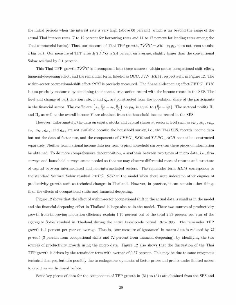
the initial periods when the interest rate is very high (above 60 percent), which is far beyond the range of the
actual Thai interest rates (7 to 12 percent for borrowing rates and 11 to 17 percent for lending rates among the
Thai commercial banks). Thus, our measure of Thai TFP growth, gTFPG = SR− sLgL, does not seem to miss
a big part. Our measure of TFP growth gTFPG is 2.4 percent on average, slightly larger than the conventional
Solow residual by 0.1 percent.
This Thai TFP growth gTFPG is decomposed into three sources: within-sector occupational-shift effect,
financial-deepening effect, and the remainder term, labeled asOCC, FIN , REM , respectively, in Figure 12. The
within-sector occupational-shift effect OCC is precisely measured. The financial-deepening effect TFPG_FIN
is also precisely measured by combining the financial transaction record with the income record in the SES. The
level and change of participation rate, p and gp, are constructed from the population share of the participants
in the financial sector. The coefficient³sY2
Π2Y2− sY1
Π1Y1
´on pgp is equal to
¡Π2Y − Π1Y
¢. The sectoral profits Π1
and Π2 as well as the overall income Y are obtained from the household income record in the SES.
However, unfortunately, the data on capital stocks and capital shares at sectoral level such as sK1 , sU1 , sK2 ,
sU2 , gK1 , gK2 , and gX2 are not available because the household survey, i.e., the Thai SES, records income data
but not the data of factor use, and the components of TFPG_SSR and TFPG_ACH cannot be constructed
separately. Neither from national income data nor from typical household surveys can these pieces of information
be obtained. To do more comprehensive decomposition, a synthesis between two types of micro data, i.e., firm
surveys and household surveys seems needed so that we may observe differential rates of returns and structure
of capital between intermediated and non-intermediated sectors. The remainder term REM corresponds to
the standard Sectoral Solow residual TFPG_SSR in the model when there were indeed no other engines of
productivity growth such as technical changes in Thailand. However, in practice, it can contain other things
than the effects of occupational shifts and financial deepening.
Figure 12 shows that the effect of within-sector occupational shift in the actual data is small as in the model
and the financial-deepening effect in Thailand is large also as in the model. These two sources of productivity
growth from improving allocation efficiency explain 1.76 percent out of the total 2.33 percent per year of the
aggregate Solow residual in Thailand during the entire two-decade period 1976-1996. The remainder TFP
growth is 1 percent per year on average. That is, “our measure of ignorance” in macro data is reduced by 75
percent (3 percent from occupational shifts and 72 percent from financial deepening), by identifying the two
sources of productivity growth using the micro data. Figure 12 also shows that the fluctuation of the Thai
TFP growth is driven by the remainder term with average of 0.57 percent. This may be due to some exogenous
technical changes, but also possibly due to endogenous dynamics of factor prices and profits under limited access
to credit as we discussed before.
Some key pieces of data for the components of TFP growth in (51) to (54) are obtained from the SES and
29

displayed in Figure 13. Observing them through the lens of the model helps us to have a deeper understanding
on the actual Thai TFP growth. The Thai wage, displayed Figure 13.1, shows a striking resemblance of the
take-off dynamics of wage in the model.18 It was surprisingly constant for the first decade before 1986 and
then grew fast for the following second decade. The only difference is that the Thai wage starts to grow earlier
in 1986 than the simulated wage does in 1990. From this, we may expect a significant contribution of wage
growth to TFPG_SSR after 1986. Figure 12 confirms this may be indeed the case: the remainder term
(which includes TFPG_SSR) surges in 1986. Note, however, that this effect would diminish as the financial
sector expands, i.e., as the effect of the profit-reduction in the credit sector and hence the tendency of decreasing
TFPG_SSR becomes larger. This provides, though not complete, one consistent explanation for the movement
of the remainder Thai TFP growth.
Figure 13.2 suggests that the interest rate of the Thai commercial banks does not show clear declining
trends, which is different from the model.19 How close this interest rate is to the “interest rate” in the model,
measuring the opportunity cost of capital as well as the marginal product of capital in the perfect credit market,
depends on how much the interest rates were regulated in Thailand. According to Alba, Hernandez, and
Klingebiel (1999), deregulation of the interest rate ceiling started in 1987 and completed by 1992. They also
report that from liberalizing the capital account began to take effects after 1986.20 This would tend to tie the
Thai interest rates to the world interest rates. Therefore, the non-declining tendency of the Thai interest rate
after 1986 seems due to the capital account liberalization, and it is due to the interest rate control before 1986.
That is, the relatively stable movement of the Thai interest rate seems to be driven by the exogenous policy
changes.
Figure 13.3 displays the average profits of non-credit and credit sectors. Before 1981, profits was stable
(only slight increase in credit sector and slight decrease in the non-credit sector). During the recession period of
1981-1986, profits declined in both sectors. After 1986 when wage started to grow, movements of profits differ
between the two sectors. In the non-credit sector, profits increased continually. In the credit sector, profits
increased fast during 1988-1992, but kept decreasing after 1992. Thus, in the non-credit sector, the profit moves
as the model predicts, but not in the credit sector.
The fraction of entrepreneurs, shown in figure 13.4, increases in the non-credit sector after 1990. The wage
growth, though with four-year lag, eventually helps the occupational shifts in the non-credit sector as the model
18The Thai wage is measured by the average wage income among the full-time wage-earning households, excluding the part-timewage income. This is normalized into the model income unit at the same scale that was used in converting the Thai baht into themodel income unit in simulation.19The interest rate series are the prime lending rates (average of the monthly values) of the four largest Thai commercial banks.
There is a spread of 3.7 percent on average between the borrowing and lending rates in Thailand, when the borrowing rate ismeasured by the average of the monthly values of the time deposit rates with maturity of more than 12 months and less than twoyears of the same banks. (Data Source: Bank of Thailand. Consistent data for these interest rates are available only from 1978.)20The ratio of foreign capital inflows to GDP surged from 2% in 1987 to 14% in 1990 and then slightly declined to 10% in 1996.
30

predicts. What is puzzling from the model’s point of view is that the fraction of entrepreneurs as well as profits
increased also in the credit sector, during this latter decade of wage growth. This suggests that the credit sector
in Thailand does not seem as perfect as in the model.
Figure 13.5 displays the sectoral wage shares in Thailand. This tells us that Thai wage share is larger in
the non-credit sector than in the credit sector, though the gap becomes smaller, again as in the model. (Recall
Figure 9.5 for the model.) Thus, the occupational-shift effect is mainly governed by the occupational shifts
non-credit sector.
These observations explain the small magnitude of the occupational-shift effect on the TFP growth (TFPG_OCC)
in Thailand. Although there is a discrepancy in the movements of interest rate between the model and the data,
the directions of the movements of the occupational shifts in response of the change in factor prices in the data
are the same with the model, except the positive response of the fraction of the entrepreneurs in the credit
sector to wage growth.
From Figure 13.4, we also know that the fraction of entrepreneurs is higher in the credit sector (21 percent
on average) than in the non-credit sector (15 percent on average), as in the model, though the model under-
predicts the fraction of entrepreneurs in the non-credit sector (1 percent) and over-predicts in the credit sector
(30 percent). Thus, expansion of the credit sector has a simple reallocation effect of increasing the fraction of
entrepreneurs in Thailand as well though its effect is smaller than the model.
The profitability gap is displayed in Figure 13.6, showing that it slightly increased until 1986, suddenly
dropped for two years when wage started to grow. Although it bounced back during 1988-1992, the gap declines
fast thereafter. This decline of profitability gap after 1992 explains the diminishing financial-deepening effect
in Thailand after 1992 in Figure 12.
In sum, the main components, occupational-shift effect (TFPG_OCC) and the financial-deepening effect
(TFPG_FIN), explain the actual Thai TFP growth as in the model. In particular, the financial-deepening
effect on TFP growth in the actual data remarkably resembles with that of the model in terms of both movements
and magnitudes, as Figure 14 shows. There seems to be an anomaly in explaining the movements of profits
and the fraction of entrepreneurs in the credit sector. The model predicts that the profits and the fraction of
entrepreneurs in the credit sector would decrease as the wage grows but it increases in the data. This suggests
that the intermediation within the credit sector seems less perfect in the data than in the model.
6.2 Capital Deepening and Financial Deepening
Although the TFP growth is an important engine of growth in Thailand (2.3 percent out of the total 7.8 percent
of output growth), the most important source of output growth in Thailand is still the capital deepening (4.5
percent out of the 7.8 percent). There are two roles of financial intermediation. First, it improves the efficiency
31

of resource allocation by channeling the funds from the people who are less productive in doing business to the
more talented but poor people, and this increases the TFP of the economy and in turn output. Our growth
accounting exercise could separate this effect out and found its importance for the TFP growth. The other
important role of financial intermediation is capital mobilization, which helps capital deepening. The growth
accounting framework cannot sort this effect of financial deepening on capital deepening out of the total capital
deepening. However, observing that the period of the acceleration of capital-deepening coincides with the period
of the acceleration of financial-deepening, shown in Figure 15, we can infer that this effect seems important in
Thailand. The contribution of the capital-deepening effect had been quite stable around 3 percent for the
first decade of 1976-1986, before the accelerated financial deepening, but it began to surge, peaking at 7.5
percent in 1991 and double on average at 6.1 percent for the latter decade of 1986-1996, after the accelerated
financial deepening. Thus, the expansion of financial sector not only directly increased the productivity of the
Thai economy but also seemed to contribute to capital deepening. It is also interesting to note that the direct
effect of financial deepening and the capital-deepening effect gradually decrease together after 1990, although
the decreasing speeds differ. Therefore, we find evidence in Thailand that productivity growth and capital
accumulation can go hand-in-hand via the same source, the financial deepening.
There remains the question of which comes first, financial deepening or capital deepening. The counterfac-
tual experiment in Giné and Townsend (2004) seems to provide an answer to this question. For the purpose of
evaluating the effect of incorporating the foreign capital inflows, they simulated the same model, adding foreign
capital into the model in the same amount as the foreign capital inflows in Thailand after 1986, while maintain-
ing the Thai financial-deepening path. Here, they found not much change in growth dynamics. However, when
the path of financial deepening is linearized, i.e., the credit sector is expanded at the same average rate of 1
percent every year without the nonlinear acceleration after 1986 (again exogenously adding the same amount of
capital), the accelerated output growth for the second decade simply vanishes and overall output growth itself
becomes lower. Thus, financial deepening seems to precede capital deepening.
7 Conclusion
The existing literature of TFP usually measures the size of TFP but rarely identifies its sources directly. The
sources of the TFP growth typically remain unknown inside the residual. We attempted to find what is inside
of the residual by integrating the model with the data and by synthesizing the micro data with the macro
data. Specifying a growth model that articulates the micro underpinnings, we brought the actual macro data
to the model to choose the parameter values that best mimic the actual aggregate output growth patterns.
Initial wealth distribution and the participation rates in the financial sector were obtained from the micro data
32
and were exogenously embedded into the model to simulate the economy. The simulated TFP growth was
decomposed into four components; occupational-shifts effect, financial-deepening effect, capital-heterogeneity
effect, and the sum of sectoral Solow residuals. Then, we brought the model back to the data and decomposed
the actual Thai TFP growth using the micro data.
In our model, households of varying talent face an imperfect credit market in financing the establishment
of business and in expanding the scale of enterprise. Thus, households are constrained by limited wealth on an
extensive margin of occupation choice and an intensive margin of capital demand, though both constraints can
be alleviated over time as wealth accumulates. The model in this paper emphasizes two important extensive
margins that create the productivity differential across sectors and activities in the economy. First, the rates
of return to the common time endowment are different across occupations. Second, the rates of return to the
capital and hence the profitability of modern firms also differ between the credit sector and the non-credit
sector. Expansion of the credit sector improves the aggregate efficiency not only directly via the second type of
profitability margin but also indirectly via the first type of occupational margin. Thus, financial deepening can
be an important source of productivity growth. The occupational shifts within each sector can also be a separate
source of productivity growth. These sources of productivity growth may well be particularly important for the
economies in transition and they can be hidden in the standard TFP growth measure.
Limited access to credit and the existence of fixed-cost capital create heterogeneity in capital. This kind of
capital heterogeneity suggests us that we use the aggregate production function with caution. In the standard
growth accounting, this capital heterogeneity effect can be hidden in TFP growth. This occurs when the
composition of the heterogeneous types of capital changes. Banerjee and Duflo (2004) discuss a broader range
of cautions on the use of aggregate production function for growth theory in various development contexts,
including credit constraints.
Applying the above methodology to Thailand, where enormous structural changes accompanied the rapid
economic growth for the two decades 1976-1996, we identify both the size and the sources of the TFP growth.
The size of the TFP growth is substantial (2.3 percent per year) in Thailand although capital accumulation is
the major source (4.5 percent per year) of the total output growth (7.8 percent per year).
It turns out that the direct contribution of the occupational shifts to the TFP growth is small in both
the model and the data. This is not because the occupational choices are unimportant but because there are
general-equilibrium forces in determining the occupational shifts, which offset each other in relation to the
endogenous movements of wage, interest rate, and profits.
It is the financial deepening, measured by the expansion of the access to credit, that directly contributes
to the TFP growth again in both the model and the data. In the actual data, financial deepening explains 75%
of the Thai TFP growth. That is, three-quarter of the “measure of our ignorance” of the Thai growth process
33

has been eliminated. Furthermore, we found that financial deepening and capital deepening go hand-in hand,
and the counterfactual experiment in Giné and Townsend (2004) suggests that financial deepening seems more
fundamental between the two.
We could address the capital-heterogeneity effect using the simulated data. This effect on the TFP growth
was large in simulation only for the short initial periods when both the level and decreasing rate of the simulated
interest rates are very high, beyond the range of Thai reality. Thus, although the existence of heterogeneity in
capital itself may well be important, the effect of the compositional changes among different kinds of capital on
the TFP growth does not seem important.
We also learned several other interesting lessons. In the model, the within-sector Solow residuals are deter-
mined by endogenous interaction between price dynamics of wage, interest rate, and profits and the evolution
of wealth distribution. This tells us two things. First, the wealth distribution clearly matters for the TFP
dynamics. Second, understanding the endogenous movements in factor prices of wage and interest rates, and
most importantly the profits, helps us to explain the fluctuation of the TFP, without necessarily incorporating
exogenous aggregate shocks.
In particular, the response of profits (as well as occupational choices) to wage growth depends on access
to credit. In the credit sector, where all decisions are fully optimal, profits should fall and cancel the wage
growth effect out. But in the non-credit sector, where wage growth helps wealth accumulation and hence the
occupational shifts of the poor but talented people, profits may go up, and reinforce the wage growth effect
on the within-sector Solow residuals. This tells us two other lessons for the growth accounting exercise. First,
observing small within-sector Solow residuals does not necessarily mean that TFP dynamics are unimportant
in each sector. Second, in doing growth accounting at any kinds of subgroup level, e.g., industry level, we have
to take the degree of limited access to credit into account in interpreting the accounting numbers, when the
wage is growing. The more intermediated is the subgroup, the less the within-group TFP growth is likely to be
observed. Of course, the differential Solow residuals across different subgroups may come from the differential
technical changes. However, as long as the access to credit is limited with varying degrees across subgroups,
differential degree of access to credit can be another source of the differences in the measured Solow residuals
across subgroups.
This paper has attempted to find a promising theory of TFP, as requested by Prescott (1998). We have
found various interesting sources of the TFP growth as above. Here, we are missing the feature of technical
changes, with which the data may well be explained better. However, shutting down the typical exogenous
technical changes was helpful in isolating these sources. Explicit use of model with a tight link to the actual
data and the synthetic use of macro and micro data were also helpful. We applied our method to Thailand and
found the importance of occupational choices and financial deepening and also the importance of the interaction
34
between endogenous price dynamics of wage, interest rate, and profits and the evolution of wealth distribution in
explaining the TFP dynamics. We expect these features are important for other countries as well, in particular,
where the limited access to credit is important and the economies are in transition.
References
[1] Abramovitz, Moses (1956), “Resource and Output Trends in the United States since 1870,” American
Economic Review, V. 46: 5-23.
[2] Alba, Pedro, Leonardo Hernandez, and Daniela Klingebiel (1999), “Financial Liberalization and the Capital
Account: Thailand, 1988-97,” Policy Research Working Paper No. 2188, World Bank.
[3] Banerjee, Abhijit, and Esther Duflo (2004), “Growth Theory Through the Lens of Development Economics,”
MIT mimeo.
[4] Banerjee, Abhijit, and Andrew Newman (1993), “Occupational Choice and Process of Development,” Jour-
nal of Political Economy V. 98: 274-298.
[5] Beck, Thorsten, Ross Levine, and Norman Loayza (2000), “Finance and the Sources of Growth,” Journal
of Financial Economics, V. 58: 261-300.
[6] Bencivenga, Valerie R., and Bruce Smith (1991), “Financial Intermediation and Endogenous Growth,”
Review of Economic Studies, V. 58: 195-209.
[7] Caselli, Francesco (2003), “The Missing Input: Accounting for Cross-Country Income Differences,” Forth-
coming in Handbook of Economic Growth, ed. by P. Aghion and S. Durlauf.
[8] Clark, Colin (1940), The Conditions of Economic Progress, London: Macmillan.
[9] Cole, Harold L., and Lee E. Ohanian (1999), “The Great Depression in the United States from a Neoclassical
Perspective,” Federal Reserve Bank of Minneapolis Quarterly Review, V. 23, No. 1: 2-24.
[10] Denison, Edward F. (1969), “Some Major Issues in Productivity Analysis: An Examination of Estimates
by Jorgenson and Griliches,” Survey of Current Business, V. 49: 1-27.
[11] Erosa, Andrés (2000), “Financial Intermediation and Occupational Choice in Development,” Review of
Economic Dynamics, V.4: 303-334.
[12] Erosa, Andrés, and Hidalgo Cabrillana (2004), “On Capital Market Imperfections as a Source of Low TFP
and Economic Rents,” mimeo.
35
[13] Fuss, Melvyn, Daniel McFadden, and Yair Mundlak (1978), “A Survey of Functional Forms in the Economic
Analysis of Production,” in Melvyn Fuss and Daniel McFadden eds., Production Economics: A Dual
Approach to Theory and Application, Amsterdam, North-Holland, Vol. 1: 219-268.
[14] Giné, Xavier, and Robert M. Townsend (2004), “Evaluation of Financial Liberalization: A General Equi-
librium Model with Constrained Occupation Choice,” Journal of Development Economics, V.74: 269-307.
[15] Goldsmith, Raymond W. (1969), Financial Structure and Development, New Haven: Yale University Press.
[16] Gollin, Douglas, Stephen L. Parente, and Richard Rogerson (2001), “Structural Transformation and Cross-
Country Income Differences,” mimeo.
[17] Greenwood, Jeremy and Jovanovic, Boyan (1990), “Financial Development, Growth, and the Distribution
of Income,” Journal of Political Economy, V. 98: 1076-1107.
[18] Griliches, Zvi (2000), R&D, Education, and Productivity, Cambridge: Harvard University Press.
[19] Hansen, Gary, and Edward C. Prescott (2002), “Malthus to Solow,” American Economic Review, V. 92:
1205-1217.
[20] Hicks, John (1965), Capital and Growth, Oxford University Press, Oxford.
[21] Hsieh, Chang-Tai (2002), “What Explains the Industrial Revolution in East Asia? Evidence from the
Factor Markets,” American Economic Review, V. 92: 502-526.
[22] Hulten, Charles R. (2001), “Total Factor Productivity: A Short Biography,” in Charles R. Hulten, Edwin
R. Dean, and Michael J. Harper eds., New Developments in Productivity Analysis, Chicago: University of
Chicago Press.
[23] Jeong, Hyeok (2000), Sources of Kuznets Dynamics in Thailand, Ph.D. Dissertation, University of Chicago.
[24] Jeong, Hyeok, and Robert M. Townsend (2003), “Growth and Inequality: Model Evaluation Based on an
Estimation-Calibration Strategy,” mimeo.
[25] Jorgenson, Dale W., and Zvi Griliches (1967), “The Explanation of Productivity Change,” Review of
Economic Studies, V. 34: 349-83.
[26] Jorgenson, Dale W., and Zvi Griliches (1972), “Issues in Growth Accounting: A Reply to Edward F.
Denison, and Final Reply,” Survey of Current Business, V. 52: 31-111, (Special Issue, The Measurement
of Productivity).
36

[27] Kehoe, Timothy J., and Edward C. Prescott (2002), “Great Depressions of the Twentieth Century,” Review
of Economic Dynamics, V. 5: 1-18.
[28] King, Robert G., and Ross Levine (1993), “Finance and Growth: Schumpeter Might Be Right,” Quarterly
Journal of Economics, V. 108: 717-737.
[29] Klenow, Peter J., and Andrés Rodríguez-Clare (1997), “The Neoclassical Revival in Growth Economics:
Has It Gone Too Far?,” NBER Macroeconomics Annual, 73-102.
[30] Kuznets, Simon (1957), “Quantitative Aspects of the Economic Growth of Nations II,” Economic Devel-
opment and Cultural Change, Supplement, V. 5: 3-111.
[31] Levine, Ross, and Sara Zervos (1998), “Stock Markets, Banks, and Economic Growth,” American Economic
Review, V. 88: 537-558.
[32] Lewis, William A. (1954), “Economic Development with Unlimited Supplies of Labor,” Manchester School
of Economics and Social Studies, V. 22: 139-191.
[33] Lloyd-Ellis, Huw. and Dan Bernhardt (2000), “Enterprise, Inequality, and Economic Development,” Review
of Economic Studies, V. 67: 147-168.
[34] Lucas, Robert E., Jr. (2002), “Life Earnings and Rural-Urban Migration,” University of Chicago, mimeo.
[35] McKinnon, Ronald I. (1973), Money and Capital in Economic Development, Washington D.C.: Brookings
Institution.
[36] Prescott, Edward C. (1998), “Needed: A Theory of Total Factor Productivity,” International Economic
Review, V.39: 525-552.
[37] Rajan, Rahuuram, and Luigi Zingales (1998), “Financial Dependence and Growth,” American Economic
Review, V. 88: 559-586.
[38] Ranis, Gustav, and John Fei (1961), “A Theory of Economic Development,” American Economic Review,
V. 51: 533-565.
[39] Schultz, Theodore W. (1988), “On Investing in Specialized Human Capital to Attain Increasing Returns,”
in The State of Development Economics, Gustav Ranis and T. Paul Schultz eds, pp. 339-52, Cambridge:
Basil Blackwell.
[40] Schultz, Theodore W. (1990), Restoring Economic Equilibrium, Cambridge: Basil Blackwell.
37
[41] Schumpeter, Joseph A. (1911), Theorie der Wirtschaftlichen Entwicklung [The Theory of Economic De-
velopment], Leipzig: Dunker & Humbolt, English Translation in 1934 by Harvard University Press.
[42] Solow, Robert M. (1957), “Technical Change and the Aggregate Production Function,” Review of Eco-
nomics and Statistics, V. 39: 312-320.
[43] Tinakorn, Pranee, and Chalongphob Sussangkarn (1994, 1998), “Productivity Growth in Thailand,” Thai-
land Development Research Institute.
[44] Townsend, Robert M. (1978), “Intermediation with Costly Bilateral Exchange,” Review of Economic Stud-
ies, V. 45: 417-425.
[45] Townsend, Robert M. (1983), “Financial Structure and Economic Activity,” American Economic Review,
V. 73: 895-911.
[46] Townsend, Robert M., and Kenichi Ueda (2004), “Financial Deepening, Inequality, and Growth: A Model-
Based Quantitative Evaluation,” mimeo.
38

A Data Appendix
A.1 Data Source
Macro data are obtained from various sources from the Thai government institutions. The series for Gross
Domestic Product (GDP) and capital stock are obtained from National Economic and Social Development
Board (NESDB), both denominated in 1988 Thai baht. The labor employment series are from Labor Force
Survey (LFS) collected by National Statistical Office (NSO). Due to the large share of agricultural sector in
Thailand, the contribution of land expansion may not be negligible. Thus, we measure the land size by the
total area of cultivated land, obtained from the Ministry of Agriculture and Cooperatives (MOAC). The factor
share data are obtained from the Thailand Development Research Institute (TDRI), documented by Tinakorn
and Sussangkarn (1994, 1998). Tinakorn and Sussangkarn (1998) use the imputed wage from Social Accounting
Matrix (SAM) with base year 1995, rather than the wage from the national income accounts, discussing the
problem of using wage income from national income accounts in Thailand. The quality of labor is adjusted by
taking wage differentials across different population groups into account (by age, gender, and education), again
following Tinakorn and Sussangkarn (1998).
The micro data on the wealth distribution, occupation choices, and financial deepening are taken from
Jeong (2000), constructed from the nationally representative household surveys, the Thai Socio-Economic Sur-
vey (SES), collected by National Statistical Office. In particular, to simulate the model economy, we need
the initial wealth distribution and the path of financial deepening that is to be exogenously embedded into
the model. The initial wealth distribution is estimated from the 1976 SES household assets data using the
principal-component analysis. See Jeong (2000) for the details of the estimation procedure. We use dichoto-
mous occupation categories as the theory suggests. The self-employed and employers in the non-agricultural
sectors are categorized as entrepreneurs. Wageworkers and farmers are categorized into wage laborers and tra-
ditional subsisters, respectively. The extent of financial deepening is measured by the rate of participation in
formal financial institutions in the Thai population. Using the SES data, we count the number of households
who actually use in the previous month any of the financial institutions: commercial banks, savings banks,
Bank for Agriculture & Agricultural Cooperative (BAAC), government housing banks, financial companies, and
credit financiers, and consider them as participants in the intermediated sector. The rest are non-participants.
A.2 Estimation of Missing Observations
The data for labor share for the years earlier than 1980 and for the final year 1996 are not available. Thus, we
fill the missing observations for labor share xt by estimating a AR(2) model:
xt = λ0 + λ1xt−1 + λ2xt−2 + εt, (63)
39
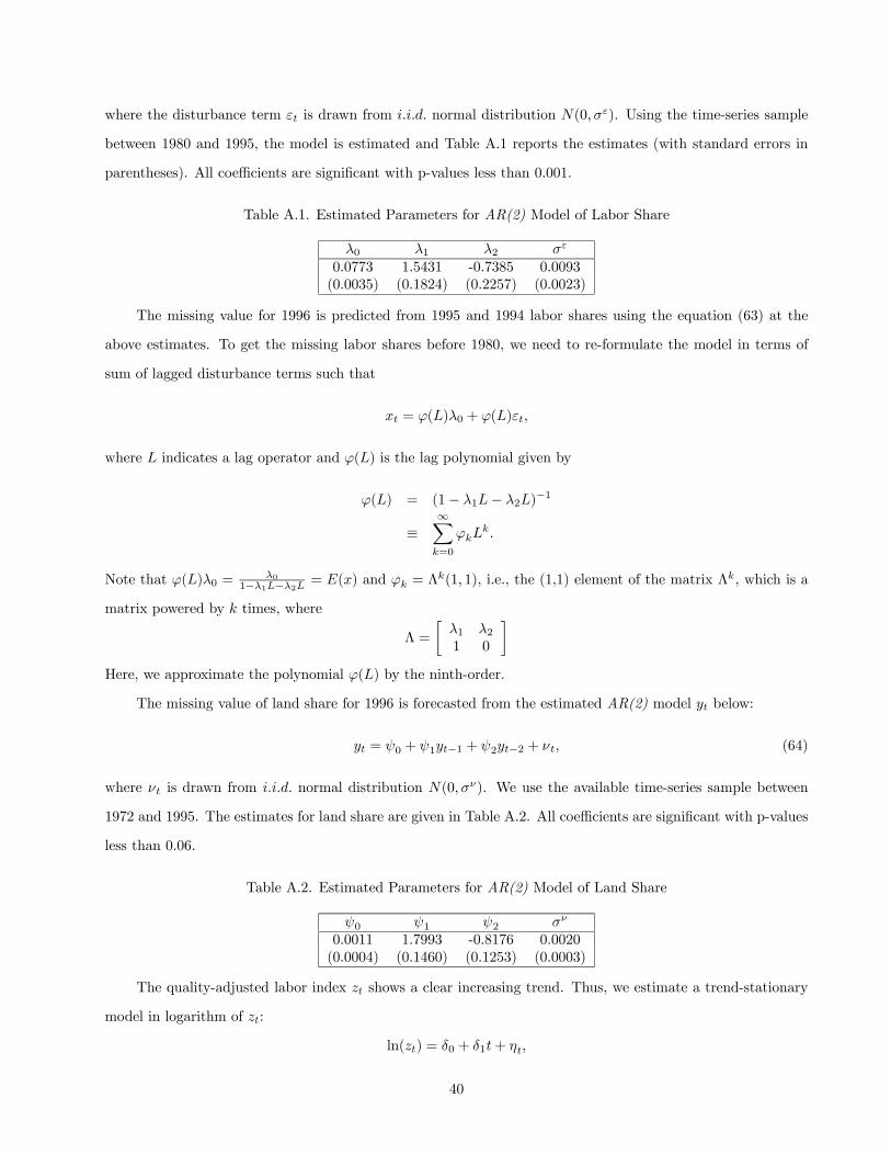
where the disturbance term εt is drawn from i.i.d. normal distribution N(0, σε). Using the time-series sample
between 1980 and 1995, the model is estimated and Table A.1 reports the estimates (with standard errors in
parentheses). All coefficients are significant with p-values less than 0.001.
Table A.1. Estimated Parameters for AR(2) Model of Labor Share
λ0 λ1 λ2 σε
0.0773 1.5431 -0.7385 0.0093(0.0035) (0.1824) (0.2257) (0.0023)
The missing value for 1996 is predicted from 1995 and 1994 labor shares using the equation (63) at the
above estimates. To get the missing labor shares before 1980, we need to re-formulate the model in terms of
sum of lagged disturbance terms such that
xt = ϕ(L)λ0 + ϕ(L)εt,
where L indicates a lag operator and ϕ(L) is the lag polynomial given by
ϕ(L) = (1− λ1L− λ2L)−1
≡∞Xk=0
ϕkLk.
Note that ϕ(L)λ0 = λ01−λ1L−λ2L = E(x) and ϕk = Λ
k(1, 1), i.e., the (1,1) element of the matrix Λk, which is a
matrix powered by k times, where
Λ =
·λ1 λ21 0
¸Here, we approximate the polynomial ϕ(L) by the ninth-order.
The missing value of land share for 1996 is forecasted from the estimated AR(2) model yt below:
yt = ψ0 + ψ1yt−1 + ψ2yt−2 + νt, (64)
where νt is drawn from i.i.d. normal distribution N(0, σν). We use the available time-series sample between
1972 and 1995. The estimates for land share are given in Table A.2. All coefficients are significant with p-values
less than 0.06.
Table A.2. Estimated Parameters for AR(2) Model of Land Share
ψ0 ψ1 ψ2 σν
0.0011 1.7993 -0.8176 0.0020(0.0004) (0.1460) (0.1253) (0.0003)
The quality-adjusted labor index zt shows a clear increasing trend. Thus, we estimate a trend-stationary
model in logarithm of zt:
ln(zt) = δ0 + δ1t+ ηt,
40
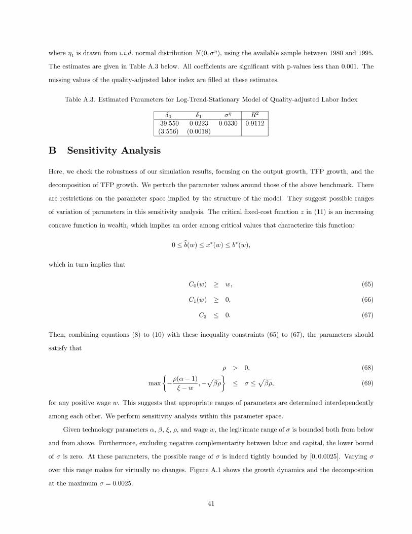
where ηt is drawn from i.i.d. normal distribution N(0, ση), using the available sample between 1980 and 1995.
The estimates are given in Table A.3 below. All coefficients are significant with p-values less than 0.001. The
missing values of the quality-adjusted labor index are filled at these estimates.
Table A.3. Estimated Parameters for Log-Trend-Stationary Model of Quality-adjusted Labor Index
δ0 δ1 ση R2
-39.550 0.0223 0.0330 0.9112(3.556) (0.0018)
B Sensitivity Analysis
Here, we check the robustness of our simulation results, focusing on the output growth, TFP growth, and the
decomposition of TFP growth. We perturb the parameter values around those of the above benchmark. There
are restrictions on the parameter space implied by the structure of the model. They suggest possible ranges
of variation of parameters in this sensitivity analysis. The critical fixed-cost function z in (11) is an increasing
concave function in wealth, which implies an order among critical values that characterize this function:
0 ≤ bb(w) ≤ x∗(w) ≤ b∗(w),
which in turn implies that
C0(w) ≥ w, (65)
C1(w) ≥ 0, (66)
C2 ≤ 0. (67)
Then, combining equations (8) to (10) with these inequality constraints (65) to (67), the parameters should
satisfy that
ρ > 0, (68)
max
½−ρ(α− 1)
ξ − w,−pβρ
¾≤ σ ≤
pβρ, (69)
for any positive wage w. This suggests that appropriate ranges of parameters are determined interdependently
among each other. We perform sensitivity analysis within this parameter space.
Given technology parameters α, β, ξ, ρ, and wage w, the legitimate range of σ is bounded both from below
and from above. Furthermore, excluding negative complementarity between labor and capital, the lower bound
of σ is zero. At these parameters, the possible range of σ is indeed tightly bounded by [0, 0.0025]. Varying σ
over this range makes for virtually no changes. Figure A.1 shows the growth dynamics and the decomposition
at the maximum σ = 0.0025.
41
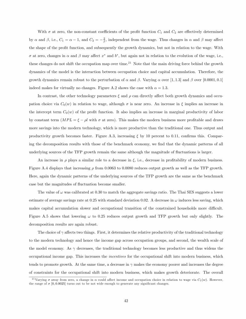
With σ at zero, the non-constant coefficients of the profit function C1 and C2 are effectively determined
by α and β, i.e., C1 = α − 1, and C2 = − 2β , independent from the wage. Thus changes in α and β may affect
the shape of the profit function, and subsequently the growth dynamics, but not in relation to the wage. With
σ at zero, changes in α and β may affect x∗ and b∗, but again not in relation to the evolution of the wage, i.e.,
these changes do not shift the occupation map over time.21 Note that the main driving force behind the growth
dynamics of the model is the interaction between occupation choice and capital accumulation. Therefore, the
growth dynamics remain robust to the perturbation of α and β. Varying α over [1, 1.3] and β over [0.0001, 0.1]
indeed makes for virtually no changes. Figure A.2 shows the case with α = 1.3.
In contrast, the other technology parameters ξ and ρ can directly affect both growth dynamics and occu-
pation choice via C0(w) in relation to wage, although σ is near zero. An increase in ξ implies an increase in
the intercept term C0(w) of the profit function. It also implies an increase in marginal productivity of labor
by constant term (MPL = ξ − ρl with σ at zero). This makes the modern business more profitable and draws
more savings into the modern technology, which is more productive than the traditional one. Thus output and
productivity growth becomes faster. Figure A.3, increasing ξ by 10 percent to 0.11, confirms this. Compar-
ing the decomposition results with those of the benchmark economy, we find that the dynamic patterns of all
underlying sources of the TFP growth remain the same although the magnitude of fluctuations is larger.
An increase in ρ plays a similar role to a decrease in ξ, i.e., decrease in profitability of modern business.
Figure A.4 displays that increasing ρ from 0.0063 to 0.0080 reduces output growth as well as the TFP growth.
Here, again the dynamic patterns of the underlying sources of the TFP growth are the same as the benchmark
case but the magnitudes of fluctuation become smaller.
The value of ω was calibrated at 0.30 to match the aggregate savings ratio. The Thai SES suggests a lower
estimate of average savings rate at 0.25 with standard deviation 0.02. A decrease in ω induces less saving, which
makes capital accumulation slower and occupational transition of the constrained households more difficult.
Figure A.5 shows that lowering ω to 0.25 reduces output growth and TFP growth but only slightly. The
decomposition results are again robust.
The choice of γ affects two things. First, it determines the relative productivity of the traditional technology
to the modern technology and hence the income gap across occupation groups, and second, the wealth scale of
the model economy. As γ decreases, the traditional technology becomes less productive and thus widens the
occupational income gap. This increases the incentives for the occupational shift into modern business, which
tends to promote growth. At the same time, a decrease in γ makes the economy poorer and increases the degree
of constraints for the occupational shift into modern business, which makes growth deteriorate. The overall
21Varying σ away from zero, a change in α could affect income and occupation choice in relation to wage via C1(w). However,the range of σ [0, 0.0025] turns out to be not wide enough to generate any significant changes.
42

effect cannot be determined a priori. However, the patterns of both growth dynamics and the decomposition
results remain robust to the perturbation of γ over [0.012, 0.025] although magnitude of fluctuations differs.
Figure A.6 displays the case of reducing γ to 0.012. Both the output and the TFP growth are accentuated
during the period of acceleration of financial expansion, but again the occupational shift effects are virtually
zero.22
22The γ value at 0.012 is chosen in the previous study by Jeong and Townsend (2003), which maximizes the likelihood ofoccupation choice of the Thai households from structural estimation.
43

0 0.2 0.4 0.6 0.8 1 1.20
0.2
0.4
0.6
0.8
11.1. Non-Credit Sector
Wealth b
Fixe
d C
ost
x
0 0.2 0.4 0.6 0.8 1 1.20
0.2
0.4
0.6
0.8
11.2. Credit Sector
Wealth b
Fixe
d C
ost
x
Figure 1. Occupation Choice
Unconstrained Subsisters & Workers
Constrained Subsisters & Workers
Constrained Entrepreneurs Unconstrained Entrepreneurs
Unconstrained Subsisters & Workers
Unconstrained Entrepreneurs
z*
x*
b̂ b*
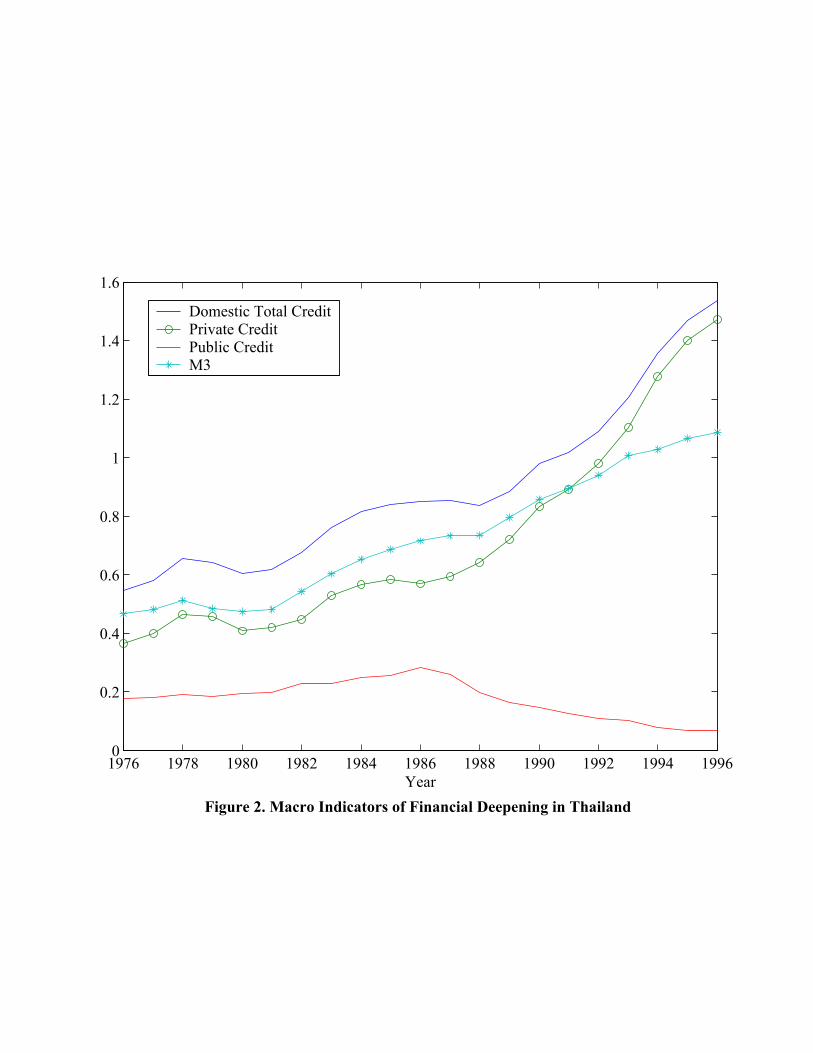
1976 1978 1980 1982 1984 1986 1988 1990 1992 1994 19960
0.2
0.4
0.6
0.8
1
1.2
1.4
1.6
Year
Domestic Total CreditPrivate CreditPublic CreditM3
Figure 2. Macro Indicators of Financial Deepening in Thailand
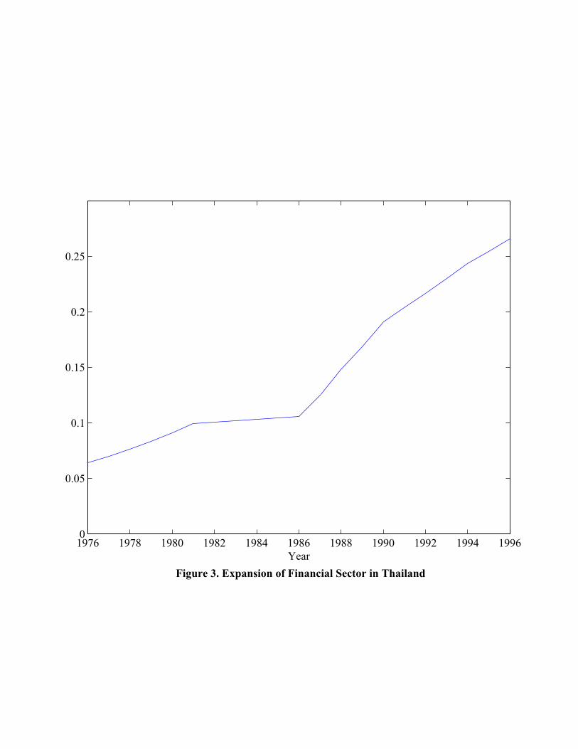
1976 1978 1980 1982 1984 1986 1988 1990 1992 1994 19960
0.05
0.1
0.15
0.2
0.25
YearFigure 3. Expansion of Financial Sector in Thailand
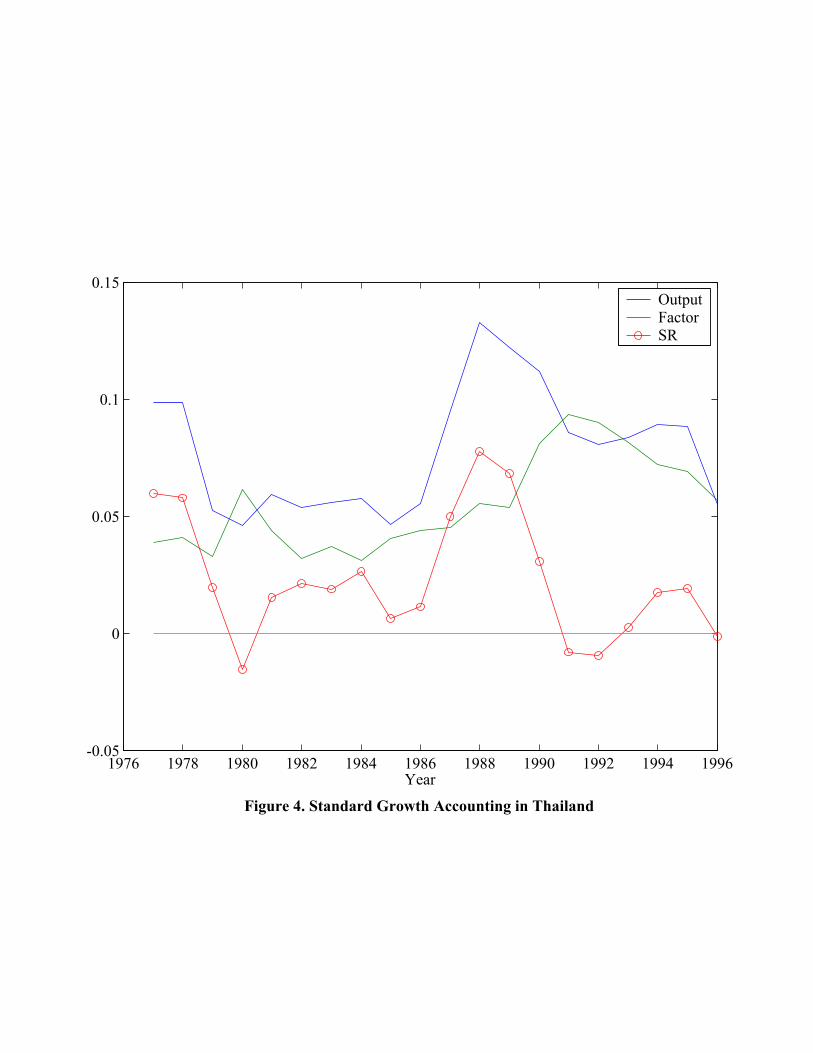
1976 1978 1980 1982 1984 1986 1988 1990 1992 1994 1996-0.05
0
0.05
0.1
0.15
Year
OutputFactorSR
Figure 4. Standard Growth Accounting in Thailand
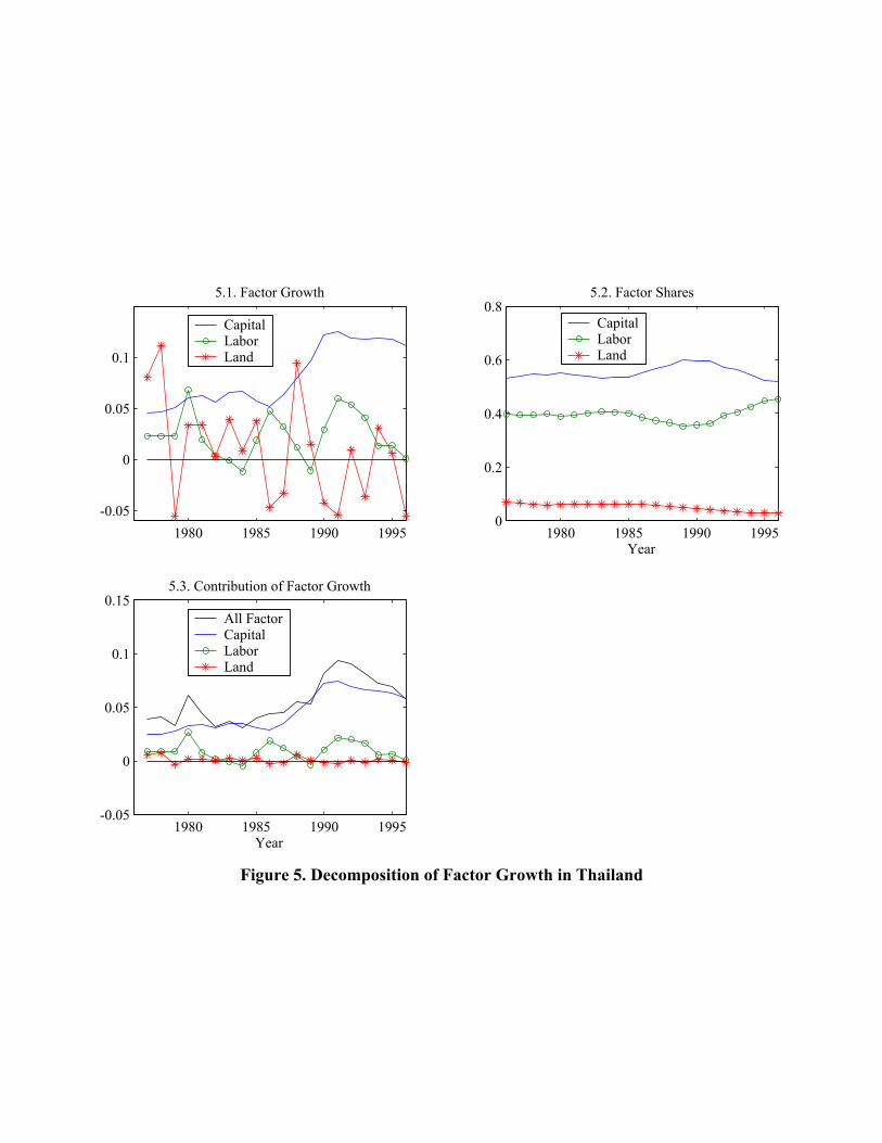
1980 1985 1990 1995-0.05
0
0.05
0.1
5.1. Factor Growth
CapitalLaborLand
1980 1985 1990 19950
0.2
0.4
0.6
0.85.2. Factor Shares
Year
CapitalLaborLand
1980 1985 1990 1995-0.05
0
0.05
0.1
0.155.3. Contribution of Factor Growth
Year
All FactorCapitalLaborLand
Figure 5. Decomposition of Factor Growth in Thailand

1976 1978 1980 1982 1984 1986 1988 1990 1992 1994 19960.1
0.15
0.2
0.25
0.3
0.35
0.4
0.45
0.5
0.55
0.6
Year
FarmerWorkerEntrepreneur
Figure 6. Occupational Transition in Thailand
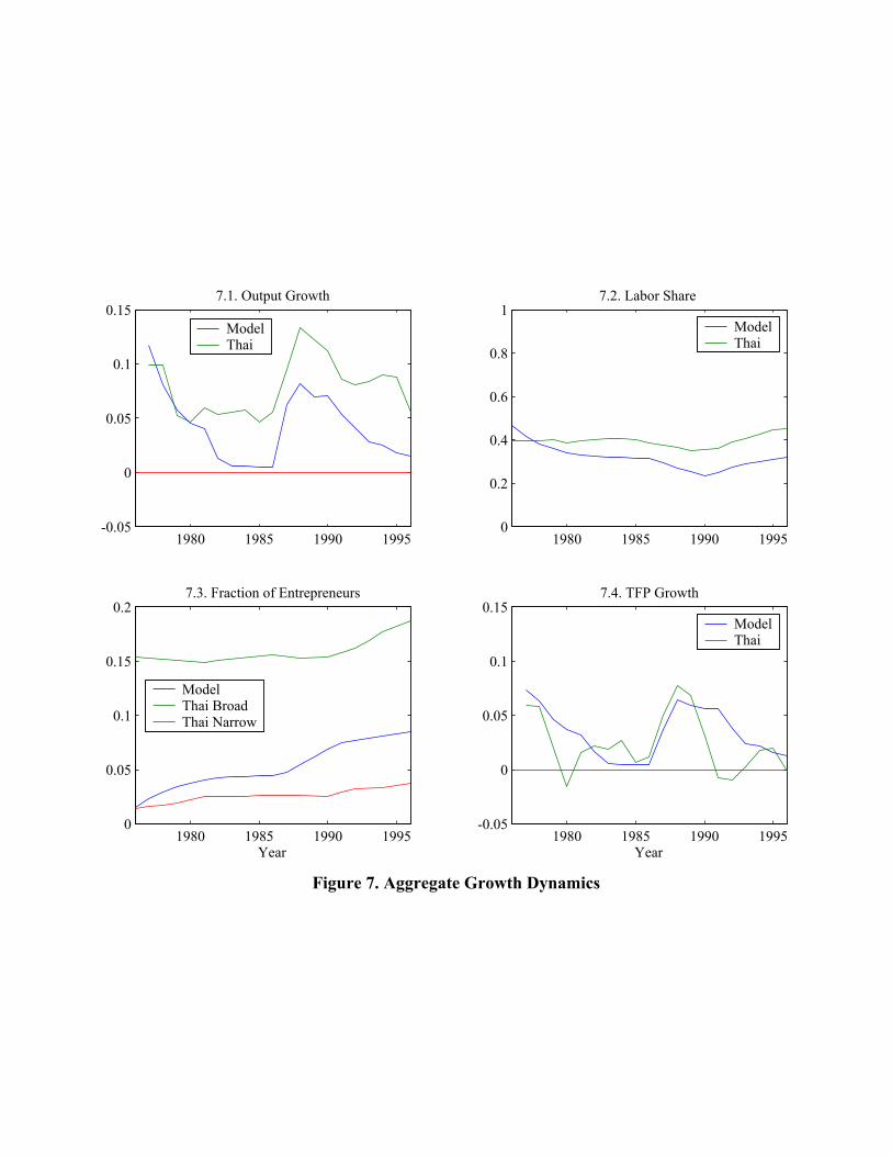
1980 1985 1990 1995-0.05
0
0.05
0.1
0.157.1. Output Growth
ModelThai
1980 1985 1990 19950
0.2
0.4
0.6
0.8
17.2. Labor Share
ModelThai
1980 1985 1990 19950
0.05
0.1
0.15
0.27.3. Fraction of Entrepreneurs
Year
ModelThai BroadThai Narrow
1980 1985 1990 1995-0.05
0
0.05
0.1
0.157.4. TFP Growth
Year
ModelThai
Figure 7. Aggregate Growth Dynamics
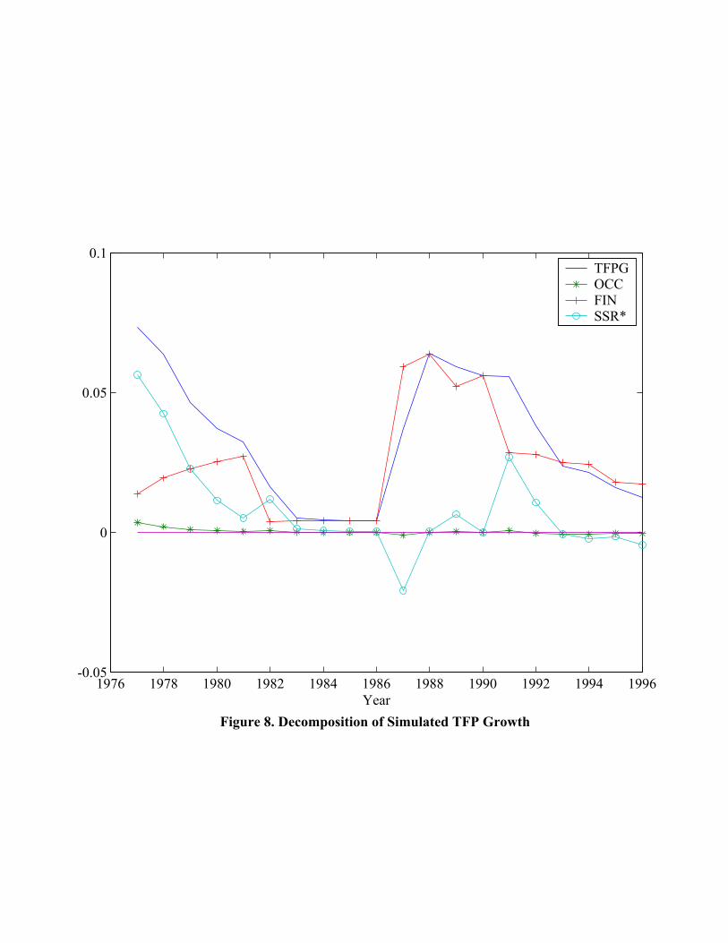
1976 1978 1980 1982 1984 1986 1988 1990 1992 1994 1996-0.05
0
0.05
0.1
Year
TFPGOCCFINSSR*
Figure 8. Decomposition of Simulated TFP Growth
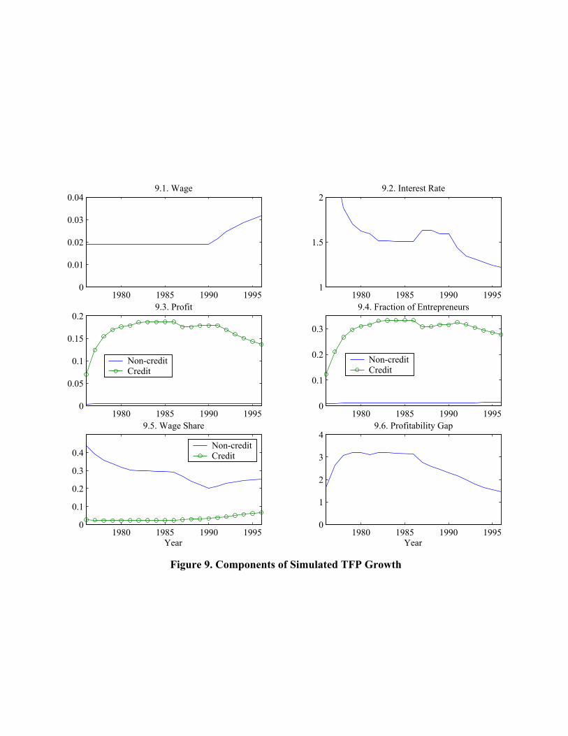
1980 1985 1990 19950
0.01
0.02
0.03
0.049.1. Wage
1980 1985 1990 19951
1.5
29.2. Interest Rate
1980 1985 1990 19950
0.05
0.1
0.15
0.29.3. Profit
Non-creditCredit
1980 1985 1990 19950
0.1
0.2
0.3
9.4. Fraction of Entrepreneurs
Non-creditCredit
1980 1985 1990 19950
0.1
0.2
0.3
0.4
9.5. Wage Share
Year
Non-creditCredit
1980 1985 1990 19950
1
2
3
49.6. Profitability Gap
Year
Figure 9. Components of Simulated TFP Growth

1976 1978 1980 1982 1984 1986 1988 1990 1992 1994 1996-0.05
0
0.05
0.1
Year
SSR*SSRACH
Figure 10. Capital-Heterogeneity Effect
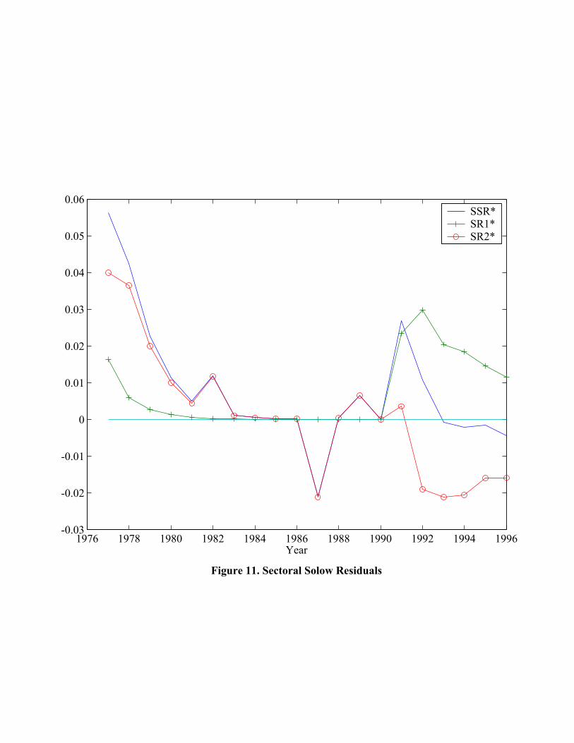
1976 1978 1980 1982 1984 1986 1988 1990 1992 1994 1996-0.03
-0.02
-0.01
0
0.01
0.02
0.03
0.04
0.05
0.06
Year
SSR*SR1*SR2*
Figure 11. Sectoral Solow Residuals
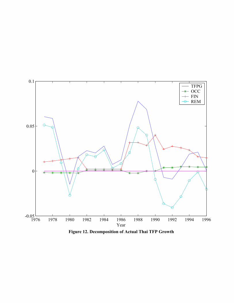
1976 1978 1980 1982 1984 1986 1988 1990 1992 1994 1996-0.05
0
0.05
0.1
Year
TFPGOCCFINREM
Figure 12. Decomposition of Actual Thai TFP Growth
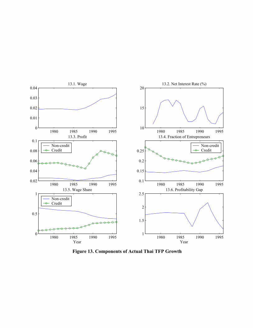
1980 1985 1990 19950
0.01
0.02
0.03
0.0413.1. Wage
1980 1985 1990 199510
15
2013.2. Net Interest Rate (%)
1980 1985 1990 19950.02
0.04
0.06
0.08
0.113.3. Profit
Non-creditCredit
1980 1985 1990 19950.1
0.15
0.2
0.25
13.4. Fraction of Entrepreneurs
Non-creditCredit
1980 1985 1990 19950
0.5
113.5. Wage Share
Year
Non-creditCredit
1980 1985 1990 19951
1.5
2
2.513.6. Profitability Gap
Year
Figure 13. Components of Actual Thai TFP Growth

1976 1978 1980 1982 1984 1986 1988 1990 1992 1994 19960
0.01
0.02
0.03
0.04
0.05
0.06
0.07
0.08
0.09
0.1
Year
ModelThai
Figure 14. TFP Growth from Financial Deepening
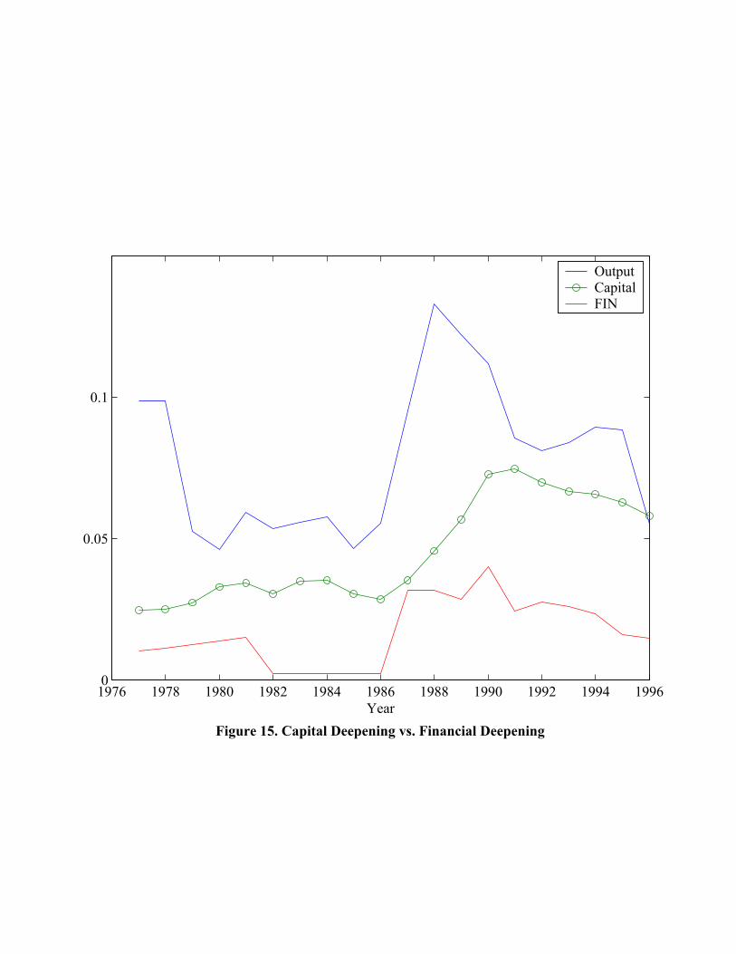
1976 1978 1980 1982 1984 1986 1988 1990 1992 1994 19960
0.05
0.1
Year
OutputCapitalFIN
Figure 15. Capital Deepening vs. Financial Deepening
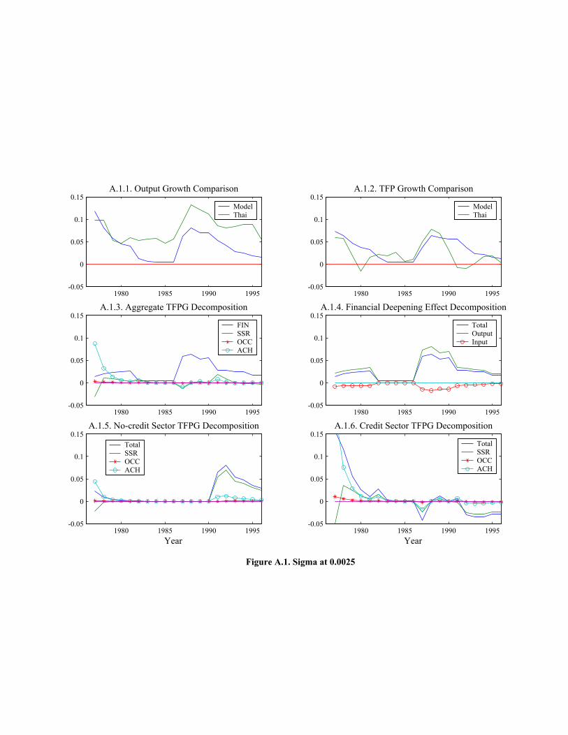
1980 1985 1990 1995-0.05
0
0.05
0.1
0.15A.1.1. Output Growth Comparison
ModelThai
1980 1985 1990 1995-0.05
0
0.05
0.1
0.15A.1.2. TFP Growth Comparison
ModelThai
1980 1985 1990 1995-0.05
0
0.05
0.1
0.15A.1.3. Aggregate TFPG Decomposition
FINSSROCCACH
1980 1985 1990 1995-0.05
0
0.05
0.1
0.15A.1.4. Financial Deepening Effect Decomposition
TotalOutputInput
1980 1985 1990 1995-0.05
0
0.05
0.1
0.15A.1.5. No-credit Sector TFPG Decomposition
Year
TotalSSROCCACH
1980 1985 1990 1995-0.05
0
0.05
0.1
0.15A.1.6. Credit Sector TFPG Decomposition
Year
TotalSSROCCACH
Figure A.1. Sigma at 0.0025

1980 1985 1990 1995-0.05
0
0.05
0.1
0.15A.2.1. Output Growth Comparison
ModelThai
1980 1985 1990 1995-0.05
0
0.05
0.1
0.15A.2.2. TFP Growth Comparison
ModelThai
1980 1985 1990 1995-0.05
0
0.05
0.1
0.15A.2.3. Aggregate TFPG Decomposition
FINSSROCCACH
1980 1985 1990 1995-0.05
0
0.05
0.1
0.15A.2.4. Financial Deepening Effect Decomposition
TotalOutputInput
1980 1985 1990 1995-0.05
0
0.05
0.1
0.15A.2.5. No-credit Sector TFPG Decomposition
Year
TotalSSROCCACH
1980 1985 1990 1995-0.05
0
0.05
0.1
0.15A.2.6. Credit Sector TFPG Decomposition
Year
TotalSSROCCACH
Figure A.2. Alpha at 1.300

1980 1985 1990 1995-0.05
0
0.05
0.1
0.15A.3.1. Output Growth Comparison
ModelThai
1980 1985 1990 1995-0.05
0
0.05
0.1
0.15A.3.2. TFP Growth Comparison
ModelThai
1980 1985 1990 1995-0.05
0
0.05
0.1
0.15A.3.3. Aggregate TFPG Decomposition
FINSSROCCACH
1980 1985 1990 1995-0.05
0
0.05
0.1
0.15A.3.4. Financial Deepening Effect Decomposition
TotalOutputInput
1980 1985 1990 1995-0.1
0
0.1
0.2
A.3.5. No-credit Sector TFPG Decomposition
Year
TotalSSROCCACH
1980 1985 1990 1995-0.1
0
0.1
0.2
A.3.6. Credit Sector TFPG Decomposition
Year
TotalSSROCCACH
Figure A.3. Xi at 0.1100
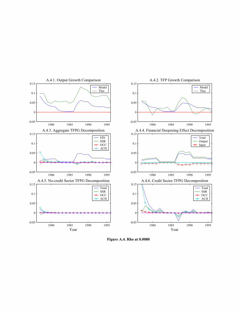
1980 1985 1990 1995-0.05
0
0.05
0.1
0.15A.4.1. Output Growth Comparison
ModelThai
1980 1985 1990 1995-0.05
0
0.05
0.1
0.15A.4.2. TFP Growth Comparison
ModelThai
1980 1985 1990 1995-0.05
0
0.05
0.1
0.15A.4.3. Aggregate TFPG Decomposition
FINSSROCCACH
1980 1985 1990 1995-0.05
0
0.05
0.1
0.15A.4.4. Financial Deepening Effect Decomposition
TotalOutputInput
1980 1985 1990 1995-0.05
0
0.05
0.1
0.15A.4.5. No-credit Sector TFPG Decomposition
Year
TotalSSROCCACH
1980 1985 1990 1995-0.05
0
0.05
0.1
0.15A.4.6. Credit Sector TFPG Decomposition
Year
TotalSSROCCACH
Figure A.4. Rho at 0.0080

1980 1985 1990 1995-0.05
0
0.05
0.1
0.15A.5.1. Output Growth Comparison
ModelThai
1980 1985 1990 1995-0.05
0
0.05
0.1
0.15A.5.2. TFP Growth Comparison
ModelThai
1980 1985 1990 1995-0.05
0
0.05
0.1
0.15A.5.3. Aggregate TFPG Decomposition
FINSSROCCACH
1980 1985 1990 1995-0.05
0
0.05
0.1
0.15A.5.4. Financial Deepening Effect Decomposition
TotalOutputInput
1980 1985 1990 1995-0.05
0
0.05
0.1
0.15A.5.5. No-credit Sector TFPG Decomposition
Year
TotalSSROCCACH
1980 1985 1990 1995-0.05
0
0.05
0.1
0.15A.5.6. Credit Sector TFPG Decomposition
Year
TotalSSROCCACH
Figure A.5. Omega at 0.25
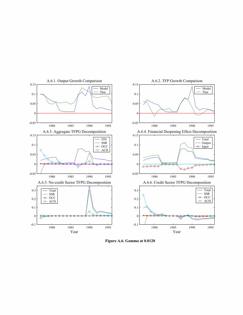
1980 1985 1990 1995-0.05
0
0.05
0.1
0.15A.6.1. Output Growth Comparison
ModelThai
1980 1985 1990 1995-0.05
0
0.05
0.1
0.15A.6.2. TFP Growth Comparison
ModelThai
1980 1985 1990 1995-0.05
0
0.05
0.1
0.15A.6.3. Aggregate TFPG Decomposition
FINSSROCCACH
1980 1985 1990 1995-0.05
0
0.05
0.1
0.15A.6.4. Financial Deepening Effect Decomposition
TotalOutputInput
1980 1985 1990 1995-0.1
0
0.1
0.2
0.3
A.6.5. No-credit Sector TFPG Decomposition
Year
TotalSSROCCACH
1980 1985 1990 1995-0.1
0
0.1
0.2
0.3
A.6.6. Credit Sector TFPG Decomposition
Year
TotalSSROCCACH
Figure A.6. Gamma at 0.0120


