Download - DISCUSSION PAPERS - La Trobe University

School of Business
Estimating a Differentiated Products Model with aDiscrete/Continuous Choice and Limited Data
DISCUSSION PAPERS
David Prentice
Series A 00.16 2000
The copyright associated with this Discussion Paper resides with theauthor(s)
Opinions expressed in this Discussion Paper are those of the author(s),not necessarily those of the School, its Departments or the University

Estimating a Differentiated Products Model with a Discrete/Continuous Choice and Limited Data
David Prentice School of Business La Trobe University
[email protected] December 1, 2000
Abstract:
This paper specifies a vertically differentiated products model for a product with a
discrete/continuous choice. The model is easily estimated with the relatively limited data
used in classical demand equation estimation, supplemented by readily available market
characteristics data. The model, with some modifications, is estimated with a new dataset
(by state and region) for the U.S. Portland cement industry. Plausible patterns of own and
cross price elasticities are obtained. The role of market characteristics is estimated
generalizing the applicability of the results to other markets and periods.
1
1. Introduction
Estimation of differentiated products models, after beginning with the U.S.
automobile industry has flowered into other consumer products (see Davis (2000) for a
recent survey). This work has developed models for particularly visibly differentiated
products, where the consumer makes a discrete choice, which are estimated with readily
available specialized datasets of prices, sales and product characteristics. Even then,
estimation remains demanding. Furthermore, for numerous products for which the
framework is appealing, useful product characteristics data is not available. One of the
implicit assumptions of the new empirical industrial organisation is that though industry
specific models are developed, they are substantially generalisable. However, the focus on
discrete choices and the specialized data and estimation requirements mean the
generalization of structural differentiated products models has been limited to date.
This paper specifies a differentiated products model for a product that features
both a discrete and continuous choice. The model is readily estimated with the type of data
typically used in classical demand equation estimation. The discrete choice component is
based on the vertical differentiation model used in Bresnahan (1987). The model is
estimated with a new dataset on U.S. state and regional Portland cement consumption,
construction, prices of building materials and other market characteristics. This dataset is
typical of data available to researchers in a broad set of products. Furthermore the model
is estimable using just instrumental variables estimation yet it yields estimates of structural
own and cross price elasticities of demand. In addition, elasticities with respect to market
characteristics are estimated.
2
This paper demonstrates how structural models of demand for differentiated
products can be extended to handle products with a discrete and continuous choice. This
case is particularly important for modeling long run demand for products, for example,
with switching costs. It is demonstrates how these models can be applied to broader set of
commodities, with more limited data, than the highly visible differentiated consumer
products considered to date. Finally, a new set of estimates of demand elasticities for
Portland cement is provided – an industry that has rarely been considered for demand
estimation (see Gupta (1975) for the only direct example).
The paper proceeds as follows. In the next section, the cement industry and the
data are introduced. At the end of this section, estimates of a set of linear demand
equations are presented, demonstrating that further structure is required to explain
demand - especially the cross-section variation. Then an estimable version of a generalized
vertical differentiation model is derived - so to handle the mixed discrete/continuous
choice and other features of the commodity and data. In section four, it is discussed how
to handle complements, uncertain substitutes and other econometric issues. Then the
estimated equations and elasticities are presented. Some suggestions for further work are
presented in the conclusion.

3
2. The Demand for Portland cement: Background, Data and Preliminary Estimates
2.1 Background
Portland cement is the powder mixed with water, sand and aggregate that makes
concrete. For a manufactured product, cement is essentially homogeneous, with no
important differences across the types of Portland cement or across the products of
different manufacturers (Prentice (1997)). Up until recently there has been no economic
substitute for cement in making concrete in the United States.
Concrete is primarily used in construction and its importance differs significantly
across different types of construction. The shares of cement in the cost of selected types of
construction are presented in Table One. Streets and Highways feature the largest share,
just over 2.5%.
Table One: Cost Share of Cement in Construction Category Percentage All Construction 0.96 New Construction 1.07 One Family Housing 1.15 Streets and Highways 2.51 Farming 1.30 Calculated by averaging requirements (including in concrete) in the Input-Output Statistics for 1972, 1977 and 1982, (Williams (1981, 1985) and Bureau of Economic Analysis (1991))
Cement differs in importance, in part, because there are several substitutes for
concrete such as asphalt, steel, wood and curtain wall products (U.S Department of
Commerce (1987)). The substitutability of concrete varies considerably with the type of
construction. While there are few substitutes for concrete for foundations and large dams,
the use of concrete varies considerably across buildings and over time. For example, the
Brutalist school, and other modernist architects made prominent and substantial use of

4
concrete in a variety of buildings (Fleming et al (1980), Jencks (1985)). In addition,
concrete houses were built in early 20th century U.S.A and Australia and are common in
developing countries today. Although cement is substantially homogeneous, it is one of a
set of differentiated products in the building materials industry, highlighted by the variety
in the buildings around us.
2.2 Highlights of the Data
In this subsection, the highlights of the data are presented. The sample is
composed of annual data on U.S. states and regions from 1956 to 1992. There are three
sets of data. First, there is the cement and construction data. Second, there is the set of
prices of building materials. Third, there is the set of market characteristics.
The characteristics of the cement and construction data are summarized in Table
Two:
Table Two: Characteristics of the Cement and Construction Data Series Aggregation Availability Sources Cement State 1956-1992 except
Hawaii, Alaska. Bureau of Mines (1956-1992)
Construction State 1967-1992, except Hawaii, Alaska.
FW Dodge
Construction Regions 1956-1966 FW Dodge NB: The components of the FW Dodge regions are listed in a Data Appendix available
from the author.
The construction data is the value of contracted new construction, supplied by
F.W. Dodge Co., which is then deflated using a construction price index constructed in
Prentice (1997). From 1956 – 1966, detailed construction data is provided for eight
regions across the U.S. From 1967 on, state level data is provided. Hence, all other data
was collected for 48 states and Washington DC for 26 years, and eight FW Dodge regions
for 11 years, providing a total of 1362 observations. The coverage of construction is not
5
complete as Preston and Lipsey (1966) suggest rural building is particularly under-
represented. Comparison with the input-output data suggests over 90% of cement
consumption is captured, but just 50-70% of new construction expenditure. However, the
FW Dodge construction data is used commercially, as a base for official statistics and is
the best available measure of detailed regional construction activity.
The quantities of construction and cement consumed are highly correlated over
time. The ratio of national cement consumption to construction, presented in Graph One,
demonstrates some cyclical variation without a trend. This is consistent with there being
no evidence of any substantial technological change in cement use in construction over the
period. This ratio is used repeatedly in the paper and is hereafter referred to as the cement-
construction ratio.
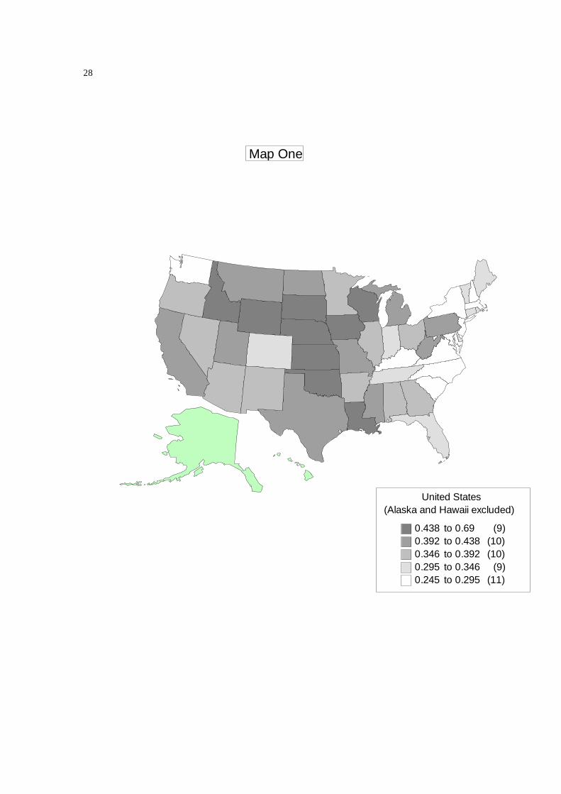
There is, though, considerable regional variation as displayed in Map One. The
plains states, and some energy producing states feature higher than average cement-
construction ratios. And the Atlantic states and Washington feature lower than average
cement-construction ratios. These differences may reflect different mixes of construction
or local prices but there is no immediate intuitive explanation for the regional variation.
In Table Three, the definitions and sources of the data on prices and market
characteristics are summarized.
The second set of data is the prices of building materials. For cement and bricks,
average prices are calculated at the source over states or a relatively small number of
states. Where prices are calculated over groups of states, these prices are assigned to all
states in the group. However, for the other substitutes, the Engineering News Record
prices are collected across twenty cities.

6
Table Three: Data Variable Definition Source
Prices of Building Materials Price-Cement Average Annual Mill Price Bureau of Mines Minerals
Yearbook (1956 – 1992) Price-Bricks Average Annual Price of
Building Bricks* Current Industrial Reports: Clay Construction Products (1957 – 1992)
Price-Steel Average – three types of Building Steel*
Engineering News Record (1956 – 1992)
Price-Lumber Average – four types of Lumber*
Engineering News Record (1956 – 1992)
Price-Gravel Average – two types of Gravel*
Engineering News Record (1956 – 1992)
Price-Asphalt Weighted average of three types of Asphalt and Road Oil.
Engineering News Record 1956 – 1969, Dept. of Energy (1970 – 1992)
Market Characteristics Disaster Prone Value of Losses for nine
types of natural disaster, by state for 1970.
Table 5.14, Petak and Atkisson (1982)
Number of Hot Days Statistical Abstract of the United States (denoted SA)
Average Temperature SA Precipitation SA Normal Minimum SA Area SA Annual Growth SA, Bureau of the Census
(1975) (denoted HS) Share of Agriculture Ratio Cash Receipts from
Farm Marketing to State Income
SA
Share of Industries Employment Share of Eight Broad Industry Groups
SA
Catch-up Ratio Ratio of Per Capita State Income to Highest Income State Income in 1950
SA, (HS)
Income Growth Growth 1950-1992 SA, (HS) Other Data
Interest Rate Real Moodys Aaa Corporate Bond Rate
Economic Report of the President. (various years)

7
Where prices are not available for states, prices from neighboring (sometimes averages
across various states) are used. All prices are deflated using the Implicit GDP Deflator,
collected from the Economic Report of the President (various years).
The third set of data is the market characteristics data. There are three sets of
characteristics: physical characteristics, economic structure and stage of development.
First, the physical characteristics of the state, including its exposure to natural disasters,
are likely to influence construction choices. For example, the demand will be lower in
states which feature both high precipitation and extreme cold as this combination of
weather makes concrete failure more likely (Lea (1970)). Demand will be higher in states
which feature short lived strong winds, like tornadoes, as concrete tends to hold well with
short-lived strong winds (Petak and Atkisson (1982)). Second, the economic structure,
and short run demand fluctuations may affect the composition of construction in ways not
captured by the different construction categories. Finally, the stage of economic growth
may also affect the composition of construction. There is no formal theory of the effects of
growth but Hayek (1939), as discussed in Montgomery (1995), suggests one pattern.
Large, basic projects are then followed by smaller more specialized projects to obtain full
value from the initial projects. Roads, dams, aqueducts are examples of basic projects
featuring cement-intensive construction.
2.3 Estimating a Standard Demand Equation
In this section, instrumental variable estimates of standard demand equations are
presented to demonstrate how they fail to adequately control for cross section variation
and to suggest issues important for modeling and estimation in sections three - five.

8
All regressions use the full sample of states and regions. The dependent variable is
the cement-construction ratio. The explanatory variables are the prices of building
materials, shares of construction types and time-varying market characteristics. As the
prices of cement and gravel are locally determined, instruments are constructed.
The first regression (not reported here), with the prices of building materials as the
sole explanatory variables, reveals this data features the heterogeneity associated with unit
record data. Prices explain just 8.6% of the variation. Hence, fixed effects are introduced
(using the within transformation to reduce multicollinearity).
In Table Four, extracts of the results of three regressions with fixed effects are
presented. The first column contains the estimates of an equation with just the prices of
building materials as explanatory variables. The second column contains the estimates of a
second equation with the prices of building materials and the shares of different types of
construction. The third column contains the estimates of a third equation with prices,
construction shares and time varying market characteristics.
Table Four: Extracts from the Demand Equation Results Explanatory Variable
Basic Specification (1)
(1) & Construction Shares
(2)
(2) & Time Varying Market
Characteristics (3)
Price – Cement -0.3706 (-7.812) -0.2286 (-5.756) -0.2180 (-5.408) Price – Brick -0.03419 (-0.361) -0.07376 (-0.947) -0.0861 (-1.112) Price – Asphalt 0.4138 (3.648) 0.5785 (5.114) 0.5938 (4.170) Price – Steel 0.1765 (3.934) 0.1928 (5.173) 0.1863 (4.974) Price – Lumber 0.0394 (1.588) 0.0624 (3.054) 0.0607 (2.947) Price – Gravel 0.2379 (1.723) 0.1347 (1.200) 0.0532 (0.469)
2R 60.04 75.71 77.26 Spearman Rank Correlation Test
23.158 19.121 10.3018
Condition Number 10.9593 1113.1 1817.55 F-Test Result 32.67 (vs. no fixed
effects) 38.19 (vs. column (1))
9.73 (vs. column (2))

9
There are two things to note about these results. First, that the coefficients on
prices have plausible signs and typically are statistically significant from zero. However,
these demand equations fail to pick up the cross sectional variation identified in Map One.
This is demonstrated by testing the relationship between the fixed effects and the
dependant variable. First, the average cement-construction ratios over time for each state
and region are calculated and ranked. Then the sizes of the fixed effects are ranked and the
two sets of ranks used in a Spearman Rank Correlation Test. In all cases the null
hypothesis of no correlation is rejected, suggesting the demand equation has failed to pick
up the cross section variation.
To gain some information on what could be determining the cross sectional
variation, the estimated fixed effects from the third specification are regressed on a set of
non-time varying explanatory variables. Extracts of the results are presented in Table Five
Table Five: Extracts of the Results of the Regression of Fixed Effects on market characteristics.
Variable Coefficient (T-Statistic) Catch-up 0.0621 (5.078) Precipitation -0.2292 (-11.339) Normal Minimum 0.3406 (5.080) Area -0.0193 (-3.516) Flood 1.1686 (13.195) Storm Surge 0.7970 (13.825) Tornado 0.0759 (1.516) Hurricane -0.6746 (-11.018) Strong Winds 11.2428 (4.048) Earthquake -0.1442 (-4.037) Landslide 0.3654 (1.396) Expansive Soil 1.0310 (17.002)
2R 71.4
A substantial proportion of the variation in the fixed effects is accounted for by the
market characteristics. Not surprisingly, weather conditions and physical disaster losses
10
influence the cement-construction ratios. Precipitation has a negative effect and strong
winds a positive effect. The catch-up variable also positively affects cement intensity,
supporting the hypothesis of Hayek (1939).
If the sole purpose of the analysis is to extract current elasticities for the cement
industry then using fixed effects is fine. However, if we want to compare elasticities across
countries or over longer periods of time, estimating the determinants of the cross section
variation is important.
3. A Structural Model of the Demand for Portland cement
In this section, an estimable differentiated products demand model featuring a
discrete and continuous choice is presented. In the first subsection, it is argued that
cement consumption is based on a mixed discrete/continuous choice. Then the discrete
choice component for each construction job is specified following the vertical
differentiation model used by Bresnahan (1987). The quantities consumed for each job are
then aggregated up to a state demand equation. This equation though features variables
unobserved by the econometrician so the equation is manipulated until an estimable
equation is obtained. Because meaningful product characteristics data does not exist,
unlike Bresnahan (1987), the estimated equation is a structural equation. To explain the
cross section variation, market characteristics are introduced as determinants of some
coefficients.
An additional complication, specific to this industry, is to allow for a price inelastic
component of the demand for cement because of building regulations or extreme physical
conditions.

11
3.1 A Model with Discrete/Continuous Product Choice and Inelastic Demand
The demand for building materials has two features that require adapting the
discrete choice framework that is the standard foundation for differentiated products
models.
The first feature is that the demand for building materials is best characterized as
featuring both a discrete choice and a continuous choice. For each component of a
construction job a discrete choice of the building material to be used must be made. For
example, the builder of a driveway could choose gravel, concrete, bricks or asphalt. This
type of choice seems not dissimilar to a choice of model of automobile or other consumer
product. However, a continuous component must be added as rather than buying one
automobile, the quantity of the chosen material varies across consumers with the size of
the construction job. It is assumed the continuous component is a linear function of the
size of the construction job i.e. in effect there is constant returns to scale in construction.
So the total quantity of the ith material consumed on a construction job, j, of type g is:
(1) conjg
ig
ijg QQ ,, β=
where igβ is the per unit requirement coefficient for input i for construction type g.
Different coefficients for different types of construction are assumed because Table One
demonstrates different construction types feature different per unit consumption of
cement. The mixed discrete/continuous specification, though required for building
materials is also applicable to other commodities, particularly those featuring switching
costs such as sunk costs before use.

12
The second modification, though, is more specific to the construction industry. It
is assumed there is a price inelastic component of demand. This is because building codes
or industry practice requires the use of concrete for some jobs because only concrete
provides, for example, sufficient strength or sealant powers. Hence there is a price
inelastic component and a price elastic component of cement consumption. Then, the total
cement consumed for a job j of type g is:
(2) ( )
−+=
otherwise chosen iscement if 1
,,
,,,,, con
jggcem
ig
conjgg
cemeg
conjgg
cemigcem
jg QkQkQk
Qβ
ββ
where kg is the share of construction type g that features a price inelastic component of
cement and cemig,β and cem
eg,β are the input requirement coefficients for the inelastic and
elastic components of cement consumption.
3.2 Modeling the Discrete Choice of a Building Material
The model of a discrete choice of a building material largely follows the adaptation
of the vertical product differentiation model in Bresnahan (1987). This model has the
disadvantage of a relatively restricted pattern of elasticities. While more general models
exist (see Davis (2000) for a survey) for the (even multiple) discrete choice case, there is
no existing model that handles the mixed discrete/continuous case required here and the
Bresnahan (1987) model can be generalized to this case relatively easily.
Therefore, we start with a model of the decision maker and then aggregate up to a
market demand equation. The decisionmaker, hereafter referred to as the client, has
income, Y, to invest and chooses one of a set of construction projects composed of
particular materials, or another investment, commonly referred to as the outside option.
Because construction is substantially an investment good rather than a consumer durable

13
the utility from the outside option is modeled as dependent on the rate of return, r, rather
than as a constant (as in Bresnahan (1987)):
(3) ( )r1YU +=
The utility gained from investing in any one of the construction projects is specified as
follows. Denote a as the taste for quality, xi as the quality of the ith material and Pi as its
price.1 The utility gained from the construction project is:
(4) ( ) ( )( )rQPYQaxQPiaYxU conjg
ig
iconjgi
conf
if
i +−+= 1,,,,,, ,, ββ
When the client chooses between the different materials, two factors are of
concern: price and quality. Quality can be thought of as an index composed of different
factors such as aesthetic appeal, strength, resistance to weather and insulation ability. It is
assumed that, for broad classes of materials, clients, following the advice of their
architects, agree on a ranking, in terms of quality, of the different materials that could be
used. But, the importance of quality is assumed to differ across clients. In particular a is
assumed to be distributed uniformly:
δdensity with ], [~ maxaaUa (Per capita).
Unlike Bresnahan (1987), the density of clients is expressed per capita rather than
absolutely. This is to allow for variations in population across the states and over time.
The taste for quality plays an important role in determining the discrete choices of
whether to invest in construction, and material to be used. For example, assume concrete
is ranked as higher quality than asphalt but of lower quality than bricks. A client is
1 The budget constraint does not enter the problem formally, but, as with Bresnahan (1987), is assumed to be satisfied. Introducing multipliers, etc., to control for the budget constraint would significantly complicate the specification without much gain.
14
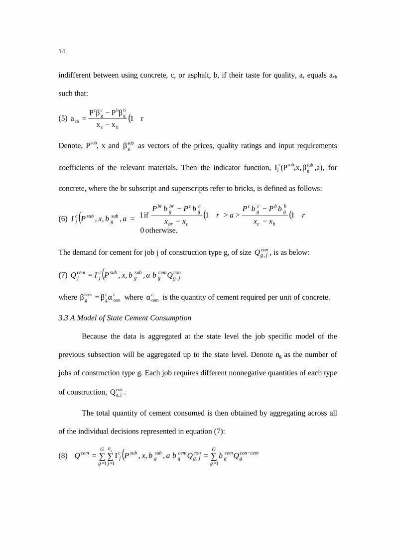
indifferent between using concrete, c, or asphalt, b, if their taste for quality, a, equals acb
such that:
(5) ( )r1xxPP
abc
bg
bcg
c
cb +−
β−β=
Denote, Psub, x and subgβ as vectors of the prices, quality ratings and input requirements
coefficients of the relevant materials. Then the indicator function, Ijc(Psub,x, sub
gβ ,a), for
concrete, where the br subscript and superscripts refer to bricks, is defined as follows:
(6) ( ) ( ) ( )
+−−
>>+−−
=otherwise. 0
11 if 1,,, rxx
PPar
xx
PPaxPI
bc
bg
bcg
c
cbr
cg
cbrg
br
subg
subcj
βββββ
The demand for cement for job j of construction type g, of size conjgQ , , is as below:
(7) ( ) conjg
cemg
subg
subcj
cemj QaxPIQ ,,,, ββ=
where ccem
cg
cemg αβ=β where c
cemα is the quantity of cement required per unit of concrete.
3.3 A Model of State Cement Consumption
Because the data is aggregated at the state level the job specific model of the
previous subsection will be aggregated up to the state level. Denote ng as the number of
jobs of construction type g. Each job requires different nonnegative quantities of each type
of construction, conj,gQ .
The total quantity of cement consumed is then obtained by aggregating across all
of the individual decisions represented in equation (7):
(8) ( )∑ ∑ ∑= =
−
==Ι=
G
g
n
j
cemcong
G
g
cemg
conjg
cemg
subg
subcj
cem g
QQaxPQ1 1 1
,,,, βββ

15
where cemcongQ − is the quantity of construction of type g that uses cement. This does not
yield an equation for estimation in terms of observable exogenous variables as cemcongQ − is
not observed. To get around this problem, first denote, congQ as the average quantity of
construction of type g and conj,gε as the deviation from the mean for job j. Then, (8) can be
rewritten as:
(9) ( ) ( )∑ ∑= =
+Ι=G
g
n
j
conjg
cong
cemg
subg
subcj
cem g
QxPQ1 1
,,, εββ
Because, for each construction type, the deviation averages out, (White (1984)), this
leaves us with (10):
(10) ( )∑ ∑= =
Ι=G
g
n
j
cong
cemg
subg
subcj
cem g
QxPQ1 1
,, ββ
Denote ng,cm as the number of projects that use cement. Equation (10) can then be
rewritten as:
(11) ∑=
=G
g
cong
cemgcmg
cem QnQ1
, β
The ng,cm, being unobservable, will now be substituted out. First, multiply and divide (11)
by ng yielding:
(12) ∑=
=
G
g
cong
cemg
g
cmgcem Qn
nQ
1
, β
Note, congQ is observable. However ng,cm and ng are not. Following Bresnahan (1987), ng,cm
for each state s can be replaced as follows:
(13) [ ] ( )
−β−β−
−β−β∗+∗∗δ=−δ=
bc
bb
cc
ca
cc
aa
sbcacscm,g xxPP
xxPP
r1popaa*pop*n
16
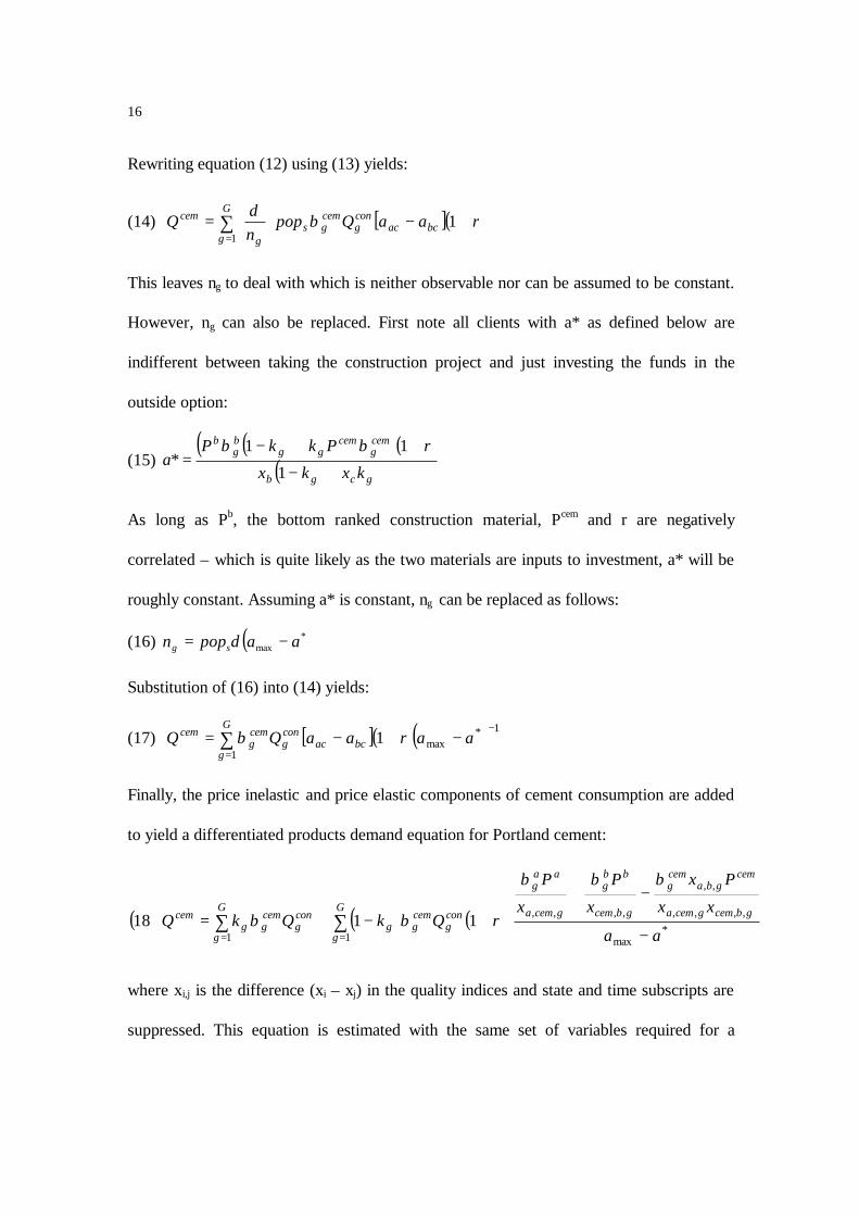
Rewriting equation (12) using (13) yields:
(14) [ ]( )raaQpopn
Q bcac
G
g
cong
cemgs
g
cem +−
= ∑
=1
1βδ
This leaves ng to deal with which is neither observable nor can be assumed to be constant.
However, ng can also be replaced. First note all clients with a* as defined below are
indifferent between taking the construction project and just investing the funds in the
outside option:
(15) ( )( )( )
( ) gcgb
cemg
cemgg
bg
b
kxkx
rPkkPa
+−++−
=1
11*
ββ
As long as Pb, the bottom ranked construction material, Pcem and r are negatively
correlated – which is quite likely as the two materials are inputs to investment, a* will be
roughly constant. Assuming a* is constant, ng can be replaced as follows:
(16) ( )∗−= aapopn sg maxδ
Substitution of (16) into (14) yields:
(17) [ ]( )( ) 1max
11
−∗
=−+−= ∑ aaraaQQ bcac
G
g
cong
cemg
cem β
Finally, the price inelastic and price elastic components of cement consumption are added
to yield a differentiated products demand equation for Portland cement:
( ) ( ) ( )∑∑= ∗=
−
−++−+=
G
g
gbcemgcema
cemgba
cemg
gbcem
bbg
gcema
aag
cong
cemgg
G
g
cong
cemgg
cem
aa
xx
Px
x
P
x
P
rQkQkQ1 max
,,,,
,,
,,,,
111 18
βββ
ββ
where xi,j is the difference (xi – xj) in the quality indices and state and time subscripts are
suppressed. This equation is estimated with the same set of variables required for a
17
classical demand equation – the prices of building materials and construction as a defacto
income. The interactive terms arise from the mixed discrete/continuous choice that forms
the foundation of the model.
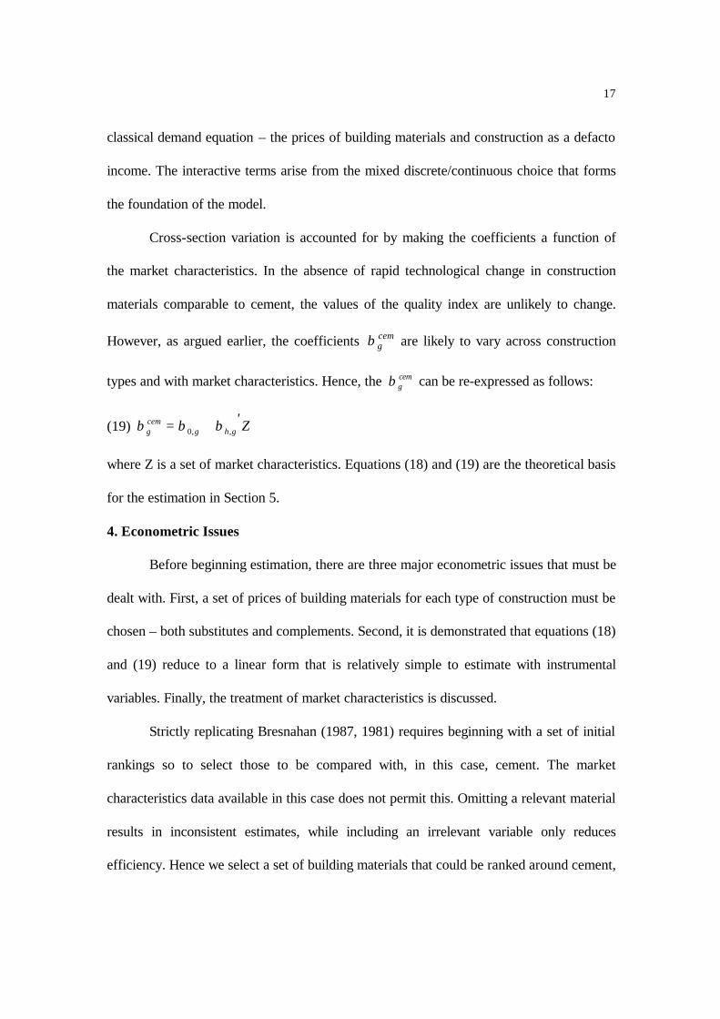
Cross-section variation is accounted for by making the coefficients a function of
the market characteristics. In the absence of rapid technological change in construction
materials comparable to cement, the values of the quality index are unlikely to change.
However, as argued earlier, the coefficients cemgβ are likely to vary across construction
types and with market characteristics. Hence, the cemgβ can be re-expressed as follows:
(19) Zghgcemg
′+= ,,0 βββ
where Z is a set of market characteristics. Equations (18) and (19) are the theoretical basis
for the estimation in Section 5.
4. Econometric Issues
Before beginning estimation, there are three major econometric issues that must be
dealt with. First, a set of prices of building materials for each type of construction must be
chosen – both substitutes and complements. Second, it is demonstrated that equations (18)
and (19) reduce to a linear form that is relatively simple to estimate with instrumental
variables. Finally, the treatment of market characteristics is discussed.
Strictly replicating Bresnahan (1987, 1981) requires beginning with a set of initial
rankings so to select those to be compared with, in this case, cement. The market
characteristics data available in this case does not permit this. Omitting a relevant material
results in inconsistent estimates, while including an irrelevant variable only reduces
efficiency. Hence we select a set of building materials that could be ranked around cement,

18
and include these in the demand equation, interacting all of them with the relevant
variables as if they were the relevant prices. The model is then supported if two of the
coefficients are significantly positive.
The related problem is that certain materials may be complementary rather than
substitutes for cement e.g. steel for reinforced concrete. Potential complements are treated
the same way as potential substitutes. They are included in the demand equation,
interacting with the relevant variables. Those inputs with coefficients significantly negative
are considered complements. Similarly, if more than two inputs prove to be significant this
suggests they are complementary to the substitutes. Ultimately, as in most estimation of
this type, the industry knowledge and judgment of the researcher will have to be relied on
to decide whether a negative coefficient is evidence of complementarity or
misspecification.
The second issue is choice of estimation technique. The model specified in
equations (18) and (19), though theoretically identified, is highly non-linear. However, the
model reduces to a linear form that retains key features and, importantly, enables
identification of the structural elasticities. The linear form estimated in section five is
summarized below:
( ) ( ) ( ) ∑ ∑∑= ==
++
=+
G
g
I
i
icongig
G
g
cong
gcon
cemg
Psr
s
rQQ
1 1,
1 11 20 θγ
(21) ggchargg Z′+= ,,0 γγγ
where congs is the share of total construction of construction type g, γ and θ are the
reduced form combinations of the structural coefficients in (18) and (19) and Ig and Zg are
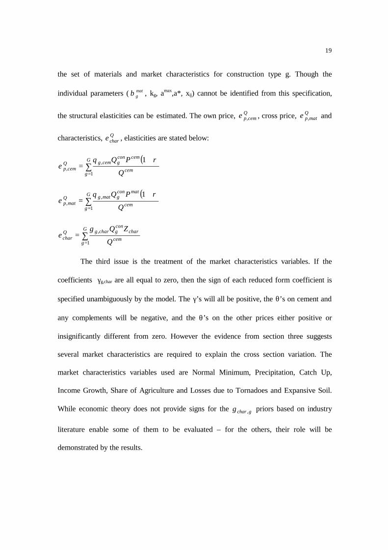
19
the set of materials and market characteristics for construction type g. Though the
individual parameters ( matgβ , kg, amax,a*, xij) cannot be identified from this specification,
the structural elasticities can be estimated. The own price, Qcemp,ε , cross price, Q
matp,ε and
characteristics, Qcharε , elasticities are stated below:
( )∑=
+=
G
gcem
cemcongcemgQ
cempQ
rPQ
1
,,
1θε
( )∑=
+=
G
gcem
matcongmatgQ
matpQ
rPQ
1
,,
1θε
∑=
=G
gcem
charcongchargQ
char Q
ZQ
1
,γε
The third issue is the treatment of the market characteristics variables. If the
coefficients γg,char are all equal to zero, then the sign of each reduced form coefficient is
specified unambiguously by the model. The γ’s will all be positive, the θ’s on cement and
any complements will be negative, and the θ’s on the other prices either positive or
insignificantly different from zero. However the evidence from section three suggests
several market characteristics are required to explain the cross section variation. The
market characteristics variables used are Normal Minimum, Precipitation, Catch Up,
Income Growth, Share of Agriculture and Losses due to Tornadoes and Expansive Soil.
While economic theory does not provide signs for the gchar ,γ priors based on industry
literature enable some of them to be evaluated – for the others, their role will be
demonstrated by the results.

20
Finally, the treatment of endogenous explanatory variables and multicollinearity is
discussed. As for the standard demand equations instruments were constructed for the
prices of cement and gravel – the building materials for which the prices were most likely
to be set locally. The other econometric problem is dealing with multicollinearity. The
results from the standard demand equation estimation suggests, suitably transformed, the
price data is not collinear but as construction and other forms of heterogeneity variables
are introduced, the interaction terms are likely to cause problems. Hence the quantity of
cement is divided by the quantity of construction and (1+r). Then all variables are centered
on their means before estimation. Finally the data is scaled to similar levels. This should
reduce problems from multicollinearity.
5. The Results
In this section, three sets of results are discussed. First, the demand equations (20)
and (21) are estimated with the gchar ,γ set equal to zero. Second, a set of elasticities
compiled from estimates of the demand equations (20) and (21) with the gchar ,γ allowed
to differ from zero are discussed. Finally, the coefficients underlying these elasticities and a
more general specification are discussed.
First, equations (20) and (21), without market characteristics, are estimated.
Though potentially inconsistent, the theoretical model provides unambiguous predictions
of the signs of the coefficients, which enables assessing, on their own terms, if the model is
supported in the data. Two versions are presented – the first with one construction type,
and the second with two types: Roads and Rest of Construction. The results are presented
in Table Six:
21
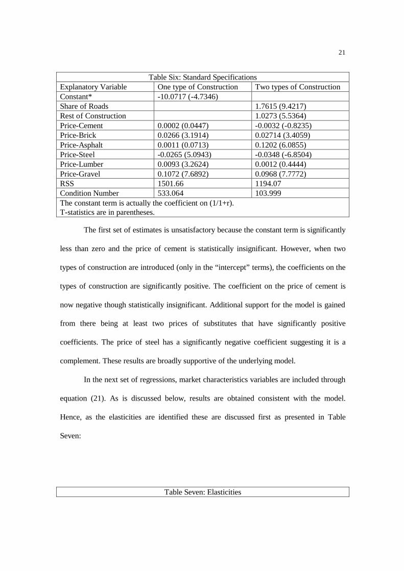
Table Six: Standard Specifications Explanatory Variable One type of Construction Two types of Construction Constant* -10.0717 (-4.7346) Share of Roads 1.7615 (9.4217) Rest of Construction 1.0273 (5.5364) Price-Cement 0.0002 (0.0447) -0.0032 (-0.8235) Price-Brick 0.0266 (3.1914) 0.02714 (3.4059) Price-Asphalt 0.0011 (0.0713) 0.1202 (6.0855) Price-Steel -0.0265 (5.0943) -0.0348 (-6.8504) Price-Lumber 0.0093 (3.2624) 0.0012 (0.4444) Price-Gravel 0.1072 (7.6892) 0.0968 (7.7772) RSS 1501.66 1194.07 Condition Number 533.064 103.999 The constant term is actually the coefficient on (1/1+r). T-statistics are in parentheses.
The first set of estimates is unsatisfactory because the constant term is significantly
less than zero and the price of cement is statistically insignificant. However, when two
types of construction are introduced (only in the “intercept” terms), the coefficients on the
types of construction are significantly positive. The coefficient on the price of cement is
now negative though statistically insignificant. Additional support for the model is gained
from there being at least two prices of substitutes that have significantly positive
coefficients. The price of steel has a significantly negative coefficient suggesting it is a
complement. These results are broadly supportive of the underlying model.
In the next set of regressions, market characteristics variables are included through
equation (21). As is discussed below, results are obtained consistent with the model.
Hence, as the elasticities are identified these are discussed first as presented in Table
Seven:
Table Seven: Elasticities

22
Prices Characteristics Variable Elasticity Variable Elasticity Cement -0.297 Normal Minimum 0.008 Brick 0.137 Precipitation -0.005 Asphalt 0.168 Catch-Up 0.015 Steel -0.122 Agriculture 0.009 Lumber -0.006 Tornado 0.004 Gravel 0.100 Income Growth 0.001 Expansive Soil 0.008
The own-price and cross price elasticities suggest relatively little substitutability
across inputs, but the pattern across inputs is quite plausible. All cross-price elasticities are
smaller than the own price elasticity. Asphalt features the largest cross price elasticity and
steel is again found to be a complement. The coefficient on lumber is statistically
insignificantly different from zero.
Next the characteristics elasticities are considered. First note that all coefficients on
the characteristics are significantly different from zero, except economic growth. But
cement demand is inelastic to small changes in these characteristics. This is not
inconsistent with the map presented earlier as the usage ratios are similar in similar states
but different across substantially different states. Catch-up is the largest, providing some
support for the pattern of growth suggested in Hayek (1939).
Next the coefficients on the two regressions with market characteristics are
presented in Table Eight. The first column (Regression One) allows for different market
characteristics to interact with the different types of construction but not the coefficients
on the prices. These results are quite successful and are used to calculate the elasticities in
Table Seven. The second set (Regression Two) allows for different coefficients on the
prices as well – but these results are less successful.
Table Eight: Coefficients
23
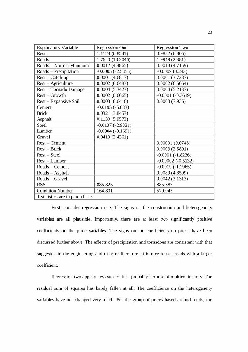
Explanatory Variable Regression One Regression Two Rest 1.1128 (6.8541) 0.9852 (6.805) Roads 1.7640 (10.2046) 1.9949 (2.381) Roads – Normal Minimum 0.0012 (4.4865) 0.0013 (4.7159) Roads – Precipitation -0.0005 (-2.5356) -0.0009 (3.243) Rest – Catch-up 0.0001 (4.6817) 0.0001 (3.7287) Rest – Agriculture 0.0002 (8.6483) 0.0002 (6.5064) Rest – Tornado Damage 0.0004 (5.3423) 0.0004 (5.2137) Rest – Growth 0.0002 (0.6665) -0.0001 (-0.3619) Rest – Expansive Soil 0.0008 (8.6416) 0.0008 (7.936) Cement -0.0195 (-5.083) Brick 0.0321 (3.8457) Asphalt 0.1130 (5.9573) Steel -0.0137 (-2.9321) Lumber -0.0004 (-0.1691) Gravel 0.0410 (3.4361) Rest – Cement 0.00001 (0.0746) Rest – Brick 0.0003 (2.5801) Rest – Steel -0.0001 (-1.8236) Rest – Lumber -0.00002 (-0.5132) Roads – Cement -0.0019 (-1.2965) Roads – Asphalt 0.0089 (4.8599) Roads – Gravel 0.0042 (3.1313) RSS 885.825 885.387 Condition Number 164.801 579.045 T statistics are in parentheses.
First, consider regression one. The signs on the construction and heterogeneity
variables are all plausible. Importantly, there are at least two significantly positive
coefficients on the price variables. The signs on the coefficients on prices have been
discussed further above. The effects of precipitation and tornadoes are consistent with that
suggested in the engineering and disaster literature. It is nice to see roads with a larger
coefficient.
Regression two appears less successful - probably because of multicollinearity. The
residual sum of squares has barely fallen at all. The coefficients on the heterogeneity
variables have not changed very much. For the group of prices based around roads, the
24
results are broadly satisfactory as both asphalt and gravel are positive and significant from
zero. Cement is negative though insignificant. However, the “rest of construction”
coefficients are less satisfactory. Cement is just insignificant but positive. Furthermore,
only brick is positive and significant, though steel remains negative and significant. These
discouraging results could be due to two causes. First, the condition number has crept up
in the second regression so multicollinearity may be starting to create problems. More
seriously, we may be coming up to the limits of what we can get out of the price data.
To summarize, these results suggest we have successfully estimated a
differentiated products model featuring a discrete/continuous choice and using largely
classical demand data. The signs of the coefficients are consistent with the theory - and
departures plausible. The pattern of elasticities is also plausible. Multicollinearity - in part
from the functional form and in part from the limits of the data - appears to be a problem.
5. Conclusions
There are ongoing important advances in estimating differentiated products
models. In general, though, these have focused on visibly differentiated consumer products
best characteristed as requiring a discrete choice. The case of a mixed discrete/continuous
case has not been considered. In this paper we develop a differentiated products model for
a product featuring a discrete and continuous choice and that is readily estimable with the
more limited data typically used in classical demand equation estimation. The model also
handles complementary products and researcher uncertainty about which inputs are
substitutes and complements. This model is estimated with a new dataset on U.S. state and
regional Portland cement consumption, prices and market characteristics. A plausible set
25
of own price and cross price elasticities are obtained. Finally, the model is easily applicable
to a broad range of products - including those with switching costs.
6. References
Bresnahan, T.F. (1981), "Departures from Marginal-cost Pricing in the American
Automobile Industry", Journal of Econometrics, 17, 201 − 227.
Bresnahan, T.F. (1987), "Competition and Collusion in the American Automobile
Industry: The 1955 Price War", Journal of Industrial Economics, 35, 457 − 482.
Bureau of the Census (1975), “Historical Statistics of the United States, colonial times to
1970”, U.S. G.P.O., Washington DC, 1975.
Bureau of Economic Analysis (1991), “The 1982 Benchmark Input-Output Accounts of
the United States”, U.S. G.P.O., Washington DC, 1991.
Bureau of Mines (1957-1992), “Minerals Yearbook” chapter on Cement. U.S Department
of the Interior, G.P.O., Washington DC.
Davis, P., (2000), "Empirical models of demand for differentiated products", European
Economic Review, 44, 993 − 1005.
Department of Energy (various years), “State Energy Price and Expenditure Report”,
Energy Information Administration, U.S. Department of Energy, G.P.O.,
Washington DC.
Fleming J., H. Honour, N. Pevsner (1980), “The Penguin Dictionary of Architecture”,
Third Edition, Penguin, Harmondsworth, 1980.
Gupta, G.S. (1975), “Demand for Cement in India”, Indian Economic Journal, 22(3), 187
− 194.
Hayek, F. (1939), “Profits, Interest and Investment” Routledge & K. Paul, London, 1939.

26
Jencks, C. (1985), “Modern Movements in Architecture”, Second Edition, Penguin,
Harmondsworth, 1985.
Lea, F.M. (1970), “The Chemistry of Cement and Concrete”, Third Edition, Edward
Arnold, London, 1970.
Lipsey, R.E. and D. Preston (1966), “Source Book of Statistics Relating to Construction”,
NBER, New York, 1966.
Montgomery, M.R. (1995), ""Time-to-Build" completion patterns for nonresidential
structures, 1961-1971", Economics Letters, 48(2), 155 − 63.
Petak, W.J. and A.A. Atkisson (1982), “Natural Hazard Risk Assessment and Public
Policy”, Springer Verlag, New York, 1982.
Prentice, D. (1997), "Import Competition in the U.S Portland Cement Industry", Ph.D.
Dissertation, Yale University.
U.S. Department of Commerce (1987), "A Competitive Assessment of the U.S Cement
Industry" U.S. Dept. of Commerce − International Trade Administration. , G.P.O.,
Washington D.C., 1987.
White, H. (1984), “Asymptotic Theory for Econometricans”, Academic Press, Orlando
FL, 1984.
Williams, F.E. (1981), “An Input-Output Profile of the Construction Industry”,
Construction Review, July/August 1981, 4 – 20.
Williams, F.E. (1985), “The 1977 Input-Output Profile of the Construction Industry”,
Construction Review, July/August 1985, 5 – 19.

27
Chart One
Ratio of Cement Consumption to Construction
0.25
0.27
0.29
0.31
0.33
0.35
0.37
0.39
0.41
1955 1957 1959 1961 1963 1965 1967 1969 1971 1973 1975 1977 1979 1981 1983 1985 1987 1989 1991 1993
Year
shor
t ton
s/$
Ratio
28
United States(Alaska and Hawaii excluded)
0.438 to 0.69 (9)0.392 to 0.438 (10)0.346 to 0.392 (10)0.295 to 0.346 (9)0.245 to 0.295 (11)
Map One


