
Distributed Bayesian Algorithms
for Fault-Tolerant Event Region Detection
in Wireless Sensor Networks ∗
Bhaskar Krishnamachari1†and Sitharama Iyengar2
1 Department of Electrical Engineering - Systems
University of Southern California
Los Angeles, California
2 Department of Computer Science
Louisiana State University
Baton Rouge, Louisiana
March 8, 2003
∗This research was funded in part by DARPA-N66001-00-1-8946, ONR-N00014-01-0712, and DOE through Oak Ridge National Lab.
†Corresponding Author.
1

Abstract
We propose a distributed solution for a canonical task in wireless sensor networks
– the binary detection of interesting environmental features. We explicitly take into
account the possibility of sensor measurement faults and develop a distributed Bayesian
algorithm for detecting and correcting such faults. Theoretical analysis and simulation
results show that 85-95% of faults can be corrected using this algorithm even when as
many as 10% of the nodes are faulty.
Keywords and Phrases: Wireless Sensor Networks, Bayesian Algorithms, Fault Recog-
nition, Fault Tolerance, Event Detection.
2

1 Introduction
Wireless sensor networks are envisioned to consist of thousands of devices, each capable of
some limited computation, communication and sensing, operating in an unattended mode.
According to a recent National Research Council report, the use of such networks of em-
bedded systems ”could well dwarf previous revolutions in the information revolution” [26].
These networks are intended for a broad range of environmental sensing applications from
vehicle tracking to habitat monitoring [9, 13, 15, 26].
In general, sensor networks can be tasked to answer any number of queries about the en-
vironment [22]. We focus on one particular class of queries: determining event regions in
the environment with a distinguishable, “feature” characteristic. As an example, consider
a network of devices that are capable of sensing concentrations of some chemical X; an im-
portant query in this situation could be “Which regions in the environment have a chemical
concentration greater than λ units?” We will refer to the process of getting answers to this
type of query as event region detection.
Event region detection is useful in and of itself as a useful application of a sensor network.
While event region detection can certainly be conducted on a static sensor network, it is
worthwhile pointing out that it can also be used as a mechanism for non-uniform sensor
deployment. Information about the location of event regions can be used to move or deploy
additional sensors to these regions in order to get finer-grained information.
Wireless sensor networks are often unattended, autonomous systems with severe energy
constraints and low-end individual nodes with limited reliability. In such conditions, self-
3

organizing, energy-efficient, fault-tolerant algorithms are required for network operation.
These design themes will guide the solution proposed in this paper to the problem of event
region detection.
To our knowledge, this is the first paper to propose a solution to the fault-feature disam-
biguation problem in sensor networks. Our proposed solution, in the form of Bayesian fault-
recognition algorithms, exploits the notion that measurement errors due to faulty equipment
are likely to be uncorrelated, while environmental conditions are spatially correlated. We
show through theoretical and simulation results that the optimal threshold decision algo-
rithm we present can reduce sensor measurement faults by as much as 85 − 95% for fault
rates up to 10%.
We begin with a short introduction to some of the prior work in the area of wireless sensor
networks, before proceeding to discuss the event region detection problem and our solution
in greater detail.
1.1 Wireless Sensor Networks
A number of independent efforts have been made in recent years to develop the hardware
and software architectures needed for wireless sensing. The challenges and design principles
involved in networking these devices are discussed in a number of recent works [1, 4, 12, 13,
26]. A good recent survey of sensor networks can be found in [34].
Self-configuration and self-organizing mechanisms are needed because of the requirement of
unattended operation in uncertain, dynamic environments. Some attention has been given to
4

developing localized, distributed, self-configuration mechanisms in sensor networks [10, 20]
and studying conditions under which they are feasible [23].
Sensor networks are characterized by severe energy constraints because the nodes will often
operate with finite battery resources and limited recharging. The energy concerns can be
addressed by engineering design at all layers. It has been recognized that energy savings
can be obtained by pushing computation within the network in the form of localized and
distributed algorithms [4, 21, 22].
One of the main advantages of the distributed computing paradigm is that it adds a new
dimension of robustness and reliability to computing. Computations done by clusters of
independent processors need not be sensitive to the failure of a small portion of the network.
Wireless sensor networks are an example of large scale distributed computing systems where
fault-tolerance is important. For large scale sensor networks to be economically feasible, the
individual nodes necessarily have to be low-end inexpensive devices. Such devices are likely
to exhibit unreliable behavior. Therefore it’s important to guarantee that faulty behavior
of individual components does not affect the overall system behavior. Some of the early
work in the area of distributed sensor networks focuses on reliable routing with arbitrary
network topologies [17, 18], characterizing sensor fault modalities [5, 6], tolerating faults
while performing sensor integration [19], and tolerating faults while ensuring sensor coverage
[16]. A mechanism for detecting crash faults in wireless sensor networks is described in [25].
There has been little prior work in the literature on detecting and correcting faults in sensor
measurements in an application-specific context. We now discuss the canonical problem of
event region detection.
5

The optimal Bayesian decision algorithm we present in this paper is closely related to the
classic voting algorithms studied in distributed applications [35, 36]. The basic idea in voting
is to get a quorum of nodes to agree on an operation before commitment. In the context of
sensor networks, voting algorithms (such as unanimous voting, majority voting, m-out-of-n
voting, and plurality voting) have been recommended as a mechanism for fusing the decisions
of multi-modal sensors with low communication overhead [37].
2 Event Region Detection
Consider a wireless network of sensors placed in an operational environment. We wish to
task this network to identify the regions in the network that contain interesting features.
For example, if the sensors monitor chemical concentrations, then we want to extract the
region of the network in which these concentrations are unusually high. It is assumed that
each sensor knows its own geographical location, either through GPS, or through RF-based
beacons [27].
It is helpful to treat the trivial centralized solution to the event region detection problem
first in order to understand the shortcomings of such an approach. We could have all nodes
report their individual sensor measurements, along with their geographical location directly
to a central monitoring node. The processing to determine the event regions can then be
performed centrally. While conceptually simple, this scheme does not scale well with the
size of the network due to the communication bottlenecks and energy expenses associated
with such a centralized scheme. Hence, we would like a solution in which the nodes in an
6

event region organize themselves and perform some local processing to determine the extent
of the region. This is the approach we will take.
Even under ideal conditions this is not an easy problem to solve, due to the requirement
of a distributed, self-organized approach. However, if we take into account the possibility
of sensor measurement faults, there is an additional layer of complexity. Can unreliable
sensors decide on their own if their measurement truly indicates a high “feature” value, or
if it is a faulty measurement? In general, this is an intractable question. It is true, however,
that the sensor measurements in the operation region are spatially correlated (since many
environmental phenomena are) while sensor faults are likely to be uncorrelated. As we
establish in this paper, we can exploit such a problem structure to give us a distributed,
localized algorithm to mitigate the effect of errors in sensor measurements.
Figure 1 shows a sample scenario. In this situation, we have a grid of sensors in some
operational area. There is an event region with unusually high chemical concentrations.
Some of the sensors shown are faulty, in that they report erroneous readings.
The first step in event region detection is for the nodes to determine which sensor readings
are interesting. In general, we can think of the sensor’s measurements as a real number.
There is some prior work on systems that learn the normal conditions over time so that they
can recognize unusual event readings [28]. We will instead make the reasonable assumption
that a threshold that enables nodes to determine whether their reading corresponds to an
event has been specified with the query, or otherwise made available to the nodes during
deployment.
7
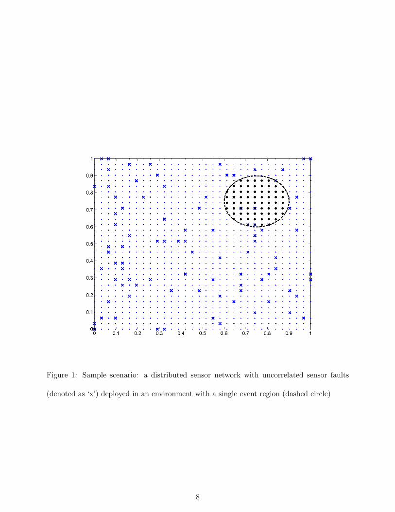
Figure 1: Sample scenario: a distributed sensor network with uncorrelated sensor faults
(denoted as ‘x’) deployed in an environment with a single event region (dashed circle)
8

A more challenging task is to disambiguate events from faults in the sensor readings, since
an unusually high reading could potentially correspond to both. Conversely, a faulty node
may report a low measurement even though it is in a event region. In this paper we present
probabilistic decoding mechanisms that exploit the fact that sensor faults are likely to be
stochastically uncorrelated, while event measurements are likely to be spatially correlated.
In analyzing these schemes, we will show that the impact of faults can be reduced by as
much as 85-95% even for reasonably high fault rates.
3 Fault-recognition
Without loss of generality, we will assume a model in which a particularly large value is
considered unusual, while the normal reading is typically a low value. If we allow for faulty
sensors, sometimes such an unusual reading could be the result of a sensor fault, rather
than an indication of the event. We assume environments in which event readings are
typically spread out geographically over multiple contiguous sensors. In such a scenario, we
can disambiguate faults from events by examining the correlation in the reading of nearby
sensors.
Let the real situation at the sensor node be modelled by a binary variable Ti. This variable
Ti = 0 if the ground truth is that the node is a normal region, and Ti = 1 if the ground truth
is that the node is in a event region. We map the real output of the sensor into an abstract
binary variable Si. This variable Si = 0 if the sensor measurement indicates a normal value,
and a Si = 1 if it measures an unusual value.
9
There are thus four possible scenarios: Si = 0, Ti = 0 (sensor correctly reports a normal
reading), Si = 0, Ti = 1 (sensor faultily reports a normal reading), Si = 1, Ti = 1 (sensor
correctly reports an unusual/event reading), and Si = 1, Ti = 0 (sensor faultily reports an
unusual reading). While each node is aware of the value of Si, in the presence of a significant
probability of a faulty reading, it can happen that Si 6= Ti. We describe below a Bayesian
fault-recognition algorithm to determine an estimate Ri of the true reading Ti after obtaining
information about the sensor readings of neighboring sensors.
In our discussions, we will make one simplifying assumption: the sensor fault probability p
is uncorrelated and symmetric. In other words,
P (Si = 0|Ti = 1) = P (Si = 1|Ti = 0) = p (1)
The binary model can result from placing a threshold on the real-valued readings of sensors.
Let mn be the mean normal reading and mf the mean event reading for a sensor. A reasonable
threshold for distinguishing between the two possibilities would be 0.5(mn+mf ). If the errors
due to sensor faults and the fluctuations in the environment can be modelled by Gaussian
distributions with mean 0 and a standard deviation σ, the fault probability p would indeed
be symmetric. It can be evaluated using the tail probability of a Gaussian, the Q-function,
as follows:
p = Q
((0.5(mf + mn)−mn)
σ
)= Q
(mf −mn
2σ
)(2)
10
We know that the Q-function decreases monotonically. Hence (2) tells us that the fault
probability is higher when (mf −mn) is low, when the mean normal and feature readings are
not sufficiently distinguishable, or when the standard deviation σ of the sensor measurement
errors. The assumption that sensor failures are uncorrelated is a standard, reasonable as-
sumption because these failures are primarily due to imperfections in manufacturing and not
a function of the nodes’ spatial deployment. The algorithms and analysis presented in this
paper may be extended to non-symmetric errors in a straightforward manner; the symmetry
assumption is made primarily for ease of exposition.
We also wish to model the spatial correlation of feature values. Let each node i have N
neighbors (excluding itself). Let’s say the evidence Ei(a, k) is that k of the neighboring
sensors report the same binary reading a as node i , while N − k of them report the reading
¬a, then we can decode according to the following model for using the evidence:
P (Ri = a|Ei(a, k)) =k
N(3)
Note that in networks that are deployed with high densities, nearby sensors are likely to
have similar event readings, unless they are at the boundary of the event region. In this
model, we have that a sensor gives equal weight to the evidence from each neighbor. More
sophisticated models may be possible, but this model commends itself as a robust mechanism
for unforseen environments.
Now, the task for each sensor is to determine a value for Ri given information about its
own sensor reading Si and the evidence Ei(a, k) regarding the readings of its neighbors. The
11

following Bayesian calculations provide the answer:
P (Ri = a|Si = b, Ei(a, k)) =P (Ri = a, Si = b|Ei(a, k))
P (Si = b|Ei(a, k))
=P (Si = b|Ri = a)P (Ri = a|Ei(a, k))
P (Si = b|Ri = a)P (Ri = a|Ei(a, k)) + P (Si = b|Ri = ¬a)P (Ri = ¬a|Ei(a, k))
≈ P (Si = b|Ti = a)P (Ri = a|Ei(a, k))
P (Si = b|Ti = a)P (Ri = a|Ei(a, k)) + P (Si = b|Ti = ¬a)P (Ri = ¬a|Ei(a, k))
(4)
Where the last relation follows from the fact that Ri is meant to be an estimate of Ti. Thus
we have for the two cases (b = a), (b = ¬a):
Paak = P (Ri = a|Si = a, Ei(a, k)) =(1− p) k
N
(1− p) kN
+ p(1− kN
)
=(1− p)k
(1− p)k + p(N − k)(5)
P (Ri = ¬a|Si = a, Ei(a, k)) = 1− P (Ri = a|Si = a, Ei(a, k))
=p(N − k)
(1− p)k + p(N − k)(6)
Equations (5), (6) show the statistic with which the sensor node can now make a decision
about whether or not to disregard its own sensor reading Si in the face of the evidence
Ei(a, k) from its neighbors.
Each node could incorporate randomization and announce if its sensor reading is correct
with probability Paak. We will refer to this as the randomized decision scheme.
An alternative is a threshold decision scheme, which uses a threshold 0 < Θ < 1 as follows:
12

if P (Ri = a|Si = a, Ei(a, k)) > Θ, then Ri is set to a, and the sensor believes that its sensor
reading is correct. If the metric is less than the threshold, then node i decides that its sensor
reading is faulty and sets Ri to ¬a.
The detailed steps of both schemes are depicted in table 1, along with the optimal threshold
decision scheme which we will discuss later in the analysis. It should be noted that with
either the randomized decision scheme or the threshold decision scheme, the relations in 5
and 6 permit the node to also indicate its confidence in the assertion that Ri = a.
We now proceed with an analysis of these decoding mechanisms for recognizing and correcting
faulty sensor measurements.
4 Analysis of Fault-recognition algorithm
In order to simplify the analysis of the Bayesian fault-recognition mechanisms, we will make
the assumption that for all N neighbors of node i, the ground truth is the same. In other
words, if node i is in a feature region, so are all its neighbors; and if i is not in a feature
region, neither are any of its neighbors. This assumption is valid everywhere except at nodes
which lie on the boundary of a feature region. For sensor networks with high density, this is
a reasonable assumption as the number of such boundary nodes will be relatively small. We
will first present results for the randomized decision scheme.
Let gk be the probability that exactly k of node i’s N neighbors are not faulty. This proba-
bility is the same irrespective of the value of Ti. This can be readily verified:
13

Randomized Decision Scheme
1. Obtain the sensor readings Sj of all Ni neighbors of node i.
2. Determine ki, the number of node i’s neighbors j with Sj = Si.
3. Calculate Paak = (1−p)ki
(1−p)ki+p(Ni−ki).
4. Generate a random number u ∈ (0, 1).
5. If u < Paak, set Ri = Si else set Ri = ¬Si.
Threshold Decision Scheme
1. Obtain the sensor readings Sj of all Ni neighbors of node i.
2. Determine ki, the number of node i’s neighbors j with Sj = Si.
3. Calculate Paak = (1−p)ki
(1−p)ki+p(Ni−ki).
4. If Paak > Θ, set Ri = Si, else set Ri = ¬Si.
Optimal Threshold Decision Scheme
1. Obtain the sensor readings Sj of all Ni neighbors of node i.
2. Determine ki, the number of node i’s neighbors j with Sj = Si.
3. If ki ≥ 0.5Ni, set Ri = Si, else set Ri = ¬Si.
Table 1: Decision Schemes for Fault Recognition
14

Symbol Definition
n Total number of deployed nodes.
nf Number of nodes in the feature region.
no Number of other nodes = n− nf .
N The number of neighbors of each node
Ti The binary variable indicating the ground truth at node i.
Si The binary variable indicating the sensor reading. Sensor is faulty ⇐⇒ Si = ¬Ti.
Ri The binary variable with the decoded value. Decoding is correct ⇐⇒ Ri = Ti
Ei(a, k) The event that k of node i’s N neighbors have the same sensor reading a.
Paak The conditional probablility P (Ri = a|Si = a, Ei(a, k)).
p The (symmetric) fault probability P (Si = 1|Ti = 0) = P (Si = 0|Ti = 1).
gk The probability that k of node i’s N neighbors are not faulty.
Θ The decision threshold
α The average number of errors after decoding
β The average number of errors corrected
γ The average number of errors uncorrected
δ The average number of new errors introduced
Table 2: Summary of Notation for Analysis of Fault-Recognition
15

gk =
(N
k
)P (Si = 0|Ti = 0)kP (Si = 1|Ti = 0)(N−k)
=
(N
k
)P (Si = 1|Ti = 1)kP (Si = 0|Ti = 0)(N−k)
=
(N
k
)(1− p)kp(N−k) (7)
With binary values possible for the three variables corresponding to the ground truth Ti,
the sensor measurement Si, and the decoded message Ri, there are eight possible combina-
tions. The conditional probabilities corresponding to these combinations are useful metrics
in analyzing the performance of this fault-recognition algorithm.
Consider first the probability P (Ri = 0|Si = 0, Ti = 0). This is the probability that the algo-
rithm estimates that there is no feature reading when the sensor is not faulty and indicates
that there is no feature.
P (Ri = 0|Si = 0, Ti = 0) =N∑
k=0
P (Ri = 0|Si = 0, Ti = 0, Ei(0, k)) =N∑
k=0
Paakgk (8)
In a similar manner, we can derive the following expressions for all these conditional proba-
bilities:
P (Ri = a|Si = a, Ti = a) = 1− P (Ri = ¬a|Si = a, Ti = a) =N∑
k=0
Paakgk (9)
P (Ri = ¬a|Si = ¬a, Ti = a) = 1− P (Ri = a|Si = ¬a, Ti = a) =N∑
k=0
PaakgN−k (10)
16

Figure 2: Metrics for the Bayesian fault-recognition algorithm with randomized decision
scheme (N = 4)
17

Figure 3: Metrics for the Bayesian fault-recognition algorithm with optimal threshold deci-
sion scheme (N=4)
18

These metrics suffice to answer questions such as the expected number of decoding errors α,
obtained by marginalizing over values for Si.
α = P (Ri = 1|Ti = 0)no + P (Ri = 0|Ti = 0)nf
= (1−N∑
k=0
Paak(gk − gN−k))n (11)
The reduction in the average number of errors is therefore (np− α)/np.
We can also now talk meaningfully about β, the average number of sensor faults corrected
by the Bayesian fault-recognition algorithm. The conditional probabilities in equations (9)
and (10) tell us about this metric:
β = (1−N∑
k=0
PaakgN−k)np (12)
A related metric is γ, the average number of faults uncorrected:
γ = (N∑
k=0
PaakgN−k)np (13)
The Bayesian fault-recognition algorithm has one setback - while it can help us correct sensor
faults, it may introduce new errors if the evidence from neighboring sensors is faulty. This
effect can be captured by the metric δ, the average number of new errors introduced by the
algorithm:
19

δ = P (Ri = 1|Si = 0, Ti = 0)(1− p)no + P (Ri = 0|Si = 1, Ti = 1)(1− p)nf
= (1−N∑
k=0
Paakgk)(1− p)n (14)
These metrics are shown in figure 2 with respect to the sensor fault probability p. While it
can be seen that for p < 0.1 (10% of the nodes being faulty on average), over 75% of the
faults can be corrected. However, the number of new errors introduced δ is seen to increase
steadily with the fault-rate and starts to affect the overall reduction in errors significantly
after about p = 0.1.
Let us now consider the threshold decision scheme. The following theorem tells us that we
can view the threshold scheme from an alternate perspective.
Theorem 1 The decision threshold scheme with Θ is equivalent to picking an integer kmin
such that node i decodes to a value Ri = Si = a if and only if at least kmin of its N neighbors
report the same sensor measurement a.
Proof Recall that in this scheme, Ri = a ⇐⇒ Paak > Θ. It suffices to show that Paak
increases monotonically with k, since in this case, for each Θ, there is some kmin beyond
which Ri is always set to a. We can rewrite equation (5) as follows:
Paak =(1− p)k
k(1− 2p) + pN(15)
20

The monotonicity can be shown by taking the derivative of this with respect to a continuous
version of the variable k:
⇒ d(Paak)
dk=
p(1− p)N
(k(1− 2p) + pN)2> 0 (16)
Specifically, kmin is given by the following expression, derived by relating equation (15) to
the parameter Θ:
kmin =
⌈pNΘ
1− p− (1− 2p)Θ
⌉(17)
�
The first question this previous theorem allows us to answer is how the metrics described in
equations (8)-(14) change for the decision threshold scheme. In this scheme, we have that if
k ≥ kmin of its neighbors also read the same value a, the node i decides on Ri = a. Thus, we
can replace Paak in equations (8)-(14) with a step function Uk, which is 1 for k ≥ kmin and
0 otherwise. This is equivalent to eliminating the Paak term and summing only terms with
k ≥ kmin. Thus for the decision threshold scheme we have that:
P (Ri = a|Si = a, Ti = a) = 1− P (Ri = ¬a|Si = a, Ti = a) =N∑
k=kmin
gk (18)
P (Ri = ¬a|Si = ¬a, Ti = a) = 1− P (Ri = a|Si = ¬a, Ti = a) =N∑
k=kmin
gN−k (19)
α = (1−N∑
k=kmin
(gk − gN−k))n (20)
21

β = (1−N∑
k=kmin
gN−k)np (21)
γ = (N∑
k=kmin
gN−k)np (22)
δ = (1−N∑
k=kmin
gk)(1− p)n (23)
The following is a strong result about the optimal threshold decision scheme.
Theorem 2 The optimum threshold value which minimizes α, the average number of errors
after decoding, is Θ∗ = (1− p). This threshold value corresponds to k∗min = 0.5N .
Proof As the goal is to find the kmin and Θ which minimize α, it is helpful to start with the
definition of α. From equation (23), we have that:
α = (1−N∑
k=kmin
(gk − gN−k))n
= (1−N∑
k=kmin
(N
k
)((1− p)kp(N−k) − pk(1− p)(N−k)))n (24)
We examine the behavior of the expression in the summand:
((1− p)kp(N−k) − pk(1− p)(N−k)) = pk(1− p)k(p(N−2k) − (1− p)(N−2k)) (25)
For p < 0.5, this expression is negative for N > 2k, zero for N = 2k, and positive for N < 2k.
In the expression for α, as we vary kmin by decreasing it by one at a time from N , we get
22
additional terms with negative contributions while kmin > 0.5N , and positive contributions
once kmin < 0.5N . It follows that α achieves a minimum when kmin = k∗min = 0.5N .
To determine what value of Θ this corresponds to, we can utilize equation (17). We have
that
pNΘ∗
1− p− (1− 2p)Θ∗ = 0.5N
⇒ pΘ∗ = 0.5(1− p− (1− 2p)Θ∗)
⇒ Θ∗(p− p + 0.5) = 0.5(1− p)
⇒ Θ∗ = (1− p) (26)
�
The above theorem says that the best policy for each node (in terms of minimizing α, the
average number of errors after decoding) is to accept its own sensor reading if and only if
at least half of its neighbors have the same reading. This is an intuitive result, following
from the equal-weight evidence model that we are using (equation (3)). This means that
the sensor nodes can perform an optimal decision without even having to estimate the value
of p. This makes the optimal-threshold decision scheme presented in table 1 an extremely
feasible mechanism for minimizing the effect of uncorrelated sensor faults.
23

Figure 4: A snapshot of the simulator showing the errors before and after fault-recognition
with optimal threshold (p = 0.1)
24

Figure 5: Normalized number of errors corrected and uncorrected with the optimal threshold
decision scheme
25

Figure 6: Normalized number of new errors introduced with the optimal threshold decision
scheme
26
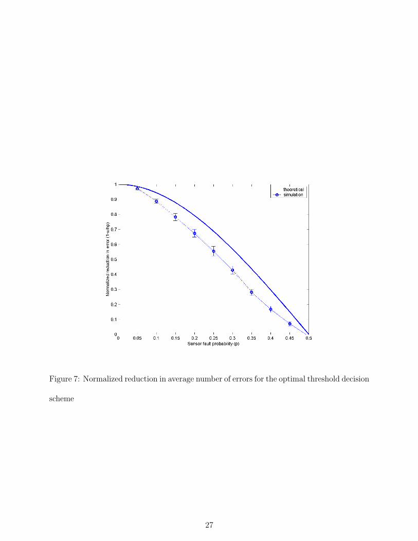
Figure 7: Normalized reduction in average number of errors for the optimal threshold decision
scheme
27

Figure 8: Normalized reduction in average number of errors with respect to the threshold
value in the threshold decision scheme (p = 0.25, Θ∗ = 1− p = 0.75)
28

Figure 9: Average fraction of errors corrected in the event region, with respect to the size of
the event region
29

5 Simulation Results
We conducted some experiments to test the performance of the fault-recognition algorithms.
The scenario consists of n = 1024 nodes placed in a 32 × 32 square grid of unit area. The
communication radius R determines which neighbors each node can communicate with. R
is set to 1√n−1
, so that each node can only communicate with its immediate neighbor in each
cardinal direction. All sensors are binary: they report a ‘0’ to indicate no feature and a ‘1’
to indicate that there is a feature. The faults are modelled by the uncorrelated, symmetric,
Bernoulli random variable. Thus each node has an independent probability p of reporting
a ‘0’ as a ‘1’ or vice versa. We model correlated features by having l single point-sources
placed in the area, and assuming that all nodes within radius S of each point-source have a
ground truth reading of 1, i.e. detect a feature if they are not faulty. For the scenario for
which the simulation results are presented here, l = 1, S = 0.15.
We now describe the simulation results. The most significant way in which the simulations
differ from the theoretical analysis that we have presented thus far is that the theoretical
analysis ignored edge and boundary effects. This can play a role because at the edge of
the deployed network, the number of neighbors per node is less than that in the interior,
and also the nodes at the edge of a feature region are more likely to erroneously determine
their reading if their neighbors provide conflicting information. Such boundary nodes are
the most likely sites of new errors introduced by the fault-recognition algorithms presented
above. In general, because of this, we would expect the number of newly introduced errors
to be higher than that predicted by the analysis.
30

Figure 4 shows a snapshot of the results of a sample simulation run. The sensor nodes are
depicted by dots; the nodes indicated with bold dots are part of the circular feature region.
An ‘x’ indicates a faulty node (before the fault-recognition algorithm), while an ‘o’ indicates
a node with erroneous readings after fault-recognition. Thus nodes with both an ‘x’ and ‘o’
are nodes whose errors were not corrected, while node with an ‘x’ but no ‘o’ are nodes whose
errors were corrected, and nodes with no ‘x’, but an ‘o’ are nodes where new error has been
introduced by the fault recognition algorithm. It can be seen that many of the remaining
errors are concentrated on the boundaries of the feature region on the top right.
Figures 5, 6, and 7, show the important performance measures for the fault recognition
algorithm with the optimal threshold decision scheme from both the simulation as well as the
theoretical equations. The key conclusion from these plots is that the simulation matches the
theoretical predictions closely in all respects except the statistic of newly introduced errors,
where understandably the border effects in the simulation result in higher values. More
concretely, these figures show that well over 85% - 95% of the total faults can be corrected
even when the fault rate is as high as 10% of the entire network.
Figure 8 illustrates the performance of the threshold decision scheme with respect to the
threshold value Θ. Again, the simulation and theoretical predictions are in close agreement.
The optimal value of the threshold Θ is indeed found to correspond to a kmin of 0.5N .
As mentioned before, many detection errors occur at the boundary of the event region.
This is because the assumption that all neighbors should have the same reading fails, by
definition, at this border. Now, the relative number of nodes a the boundary of an event
31

region (compared to the number of nodes within the region) decreases as the size of the
event region increases. We should therefore expect to see the algorithm perform better as
the event region increases. This is shown by figure 9 which measures the improvement in
the average fraction of errors corrected in the feature region.
Finally, we comment on the impact of the parameter N , the number of neighbors of each
node, on the performance of the algorithms we have proposed. There are essentially two
ways to increase N - by increasing the sensor density or by increasing the communication
range of each node. All other factors remaining the same, increasing N by increasing the
deployed density of sensors can significantly improve the performance of the algorithm. This
is because this would allow a greater sampling of a spatially correlated event. However,
increasing N by keeping the density the same and increasing the communication range can
have the opposite effect. Increasing the communication range can effectively increase the
number of nodes that are at the “boundary” of the event region – potentially increasing the
number of nodes at which incorrect decisions are made by the Bayesian algorithms. Both
these effects were observed in our simulations.
6 Conclusions
With recent advances in technology it has become feasible to consider the deployment of
large-scale wireless sensor networks that can provide high-quality environmental monitoring
for a range of applications. In this paper we developed a solution to a canonical task in such
networks – the extraction of information about regions in the environment with identifiable
32

features.
One of the most difficult challenge is that of distinguishing between faulty sensor measure-
ments and unusual environmental conditions. To our knowledge, this is the first paper to
propose a solution to the fault-feature disambiguation problem in sensor networks. Our
proposed solution, in the form of Bayesian fault-recognition algorithms, exploits the no-
tion that measurement errors due to faulty equipment are likely to be uncorrelated, while
environmental conditions are spatially correlated.
We presented two Bayesian algorithms, the randomized decision scheme and the thresh-
old decision scheme and derived analytical expressions for their performance. Our analysis
showed that the threshold decision scheme has better performance in terms of the mini-
mization of errors. We also derived the optimal setting for the threshold decision scheme
for the average-correlation model. The proposed algorithm has the additional advantage of
being completely distributed and localized - each node only needs to obtain information from
neighboring sensors in order to make its decisions. The theoretical and simulation results
show that with the optimal threshold decision scheme, faults can be reduced by as much as
85 to 95% for fault rates as high as 10%.
We should note that the extension to non-symmetric fault probabilities is straightforward and
does not affect the basic conclusions of this paper. There are a number of other directions in
which this work on fault-recognition and fault-tolerance in sensor networks can be extended.
We have dealt with a binary fault-feature disambiguation problem here. This could be
generalized to the correction of real-valued sensor measurement errors: nodes in a sensor
33

network should be able to exploit the spatial correlation of environmental readings to correct
for the noise in their readings (the noise models would be different from the binary 0-1
failures considered in this work). Another related direction is to consider dynamic sensor
faults where the same nodes need not always be faulty. Much of the work presented here can
also be extended to dynamic event region detection to deal with environmental phenomena
that change location or shape over time. We would also like to see the algorithms proposed
in this paper implemented and validated on real sensor network hardware in the near future.
34
References
[1] D. Estrin, L. Girod, G. Pottie, and M. Srivastava, “Instrumenting the World with Wireless Sen-
sor Networks,” International Conference on Acoustics, Speech and Signal Processing (ICASSP
2001), Salt Lake City, Utah, May 2001.
[2] C. Intanagonwiwat, R. Govindan and D. Estrin, “Directed Diffusion: A Scalable and Robust
Communication Paradigm for Sensor Networks,” ACM/IEEE International Conference on Mo-
bile Computing and Networks (MobiCom 2000), August 2000, Boston, Massachusetts
[3] C. Intanagonwiwat, D. Estrin, R. Govindan, and J. Heidemann, “Impact of Network Density
on Data Aggregation in Wireless Sensor Networks” , In Proceedings of the 22nd International
Conference on Distributed Computing Systems (ICDCS’02), Vienna, Austria. July, 2002.
[4] D. Estrin, R. Govindan, J. Heidemann and S. Kumar, “Next Century Challenges: Scalable
Coordination in Sensor Networks,” ACM/IEEE International Conference on Mobile Computing
and Networks (MobiCom ’99), Seattle, Washington, August 1999.
[5] K. Marzullo, “Implementing fault-tolerant sensors,” TR89-997, Dept. of Computer Science,
Cornell University, May 1989.
[6] L. Prasad, S. S. Iyengar, R. L. Kashyap, and R. N. Madan, “Functional Characterization
of Fault Tolerant Interation in Disributed Sensor Networks,” IEEE Transactions on Systems,
Man, and Cybernetics, Vol. 21, No. 5, September/October 1991.
[7] N. Lynch, Distributed Algorithms, Morgan Kauffman, 1997.
[8] B.A. Forouzan, Data Communications and Networking, McGraw Hill, 2001.
35

[9] A. Cerpa et al., “Habitat monitoring: Application driver for wireless communications technol-
ogy,” 2001 ACM SIGCOMM Workshop on Data Communications in Latin America and the
Caribbean, Costa Rica, April 2001.
[10] A. Cerpa and D. Estrin, “ASCENT: Adaptive Self-Configuring sEnsor Networks Topologies,”
INFOCOM, 2002.
[11] J. Heidemann, F. Silva, C. Intanagonwiwat, R. Govindan, D. Estrin, and D. Ganesan, “Build-
ing Efficient Wireless Sensor Networks with Low-Level Naming,” 18th ACM Symposium on
Operating Systems Principles, October 21-24, 2001.
[12] W.W. Manges, “Wireless Sensor Network Topologies,” Sensors Magazine, vol. 17, no. 5, May
2000.
[13] G.J. Pottie, W.J. Kaiser, “Wireless Integrated Network Sensors,” Communications of the
ACM, vol. 43, no. 5, pp. 551-8, May 2000.
[14] S. Singh, M. Woo, C.S. Raghavendra, “Power-aware routing in mobile ad-hoc networks,”
ACM/IEEE International Conference on Mobile Computing and Networks (MOBICOM’98),
pages 76-84, October 1999, Dallas, Texas.
[15] J. Warrior, “Smart Sensor Networks of the Future,” Sensors Magazine, March 1997.
[16] K. Chakrabarty, S. S. Iyengar, H. Qi, E.C. Cho, ” Grid Coverage of Surveillance and Target
location in Distributed Sensor Networks” To appear in IEEE Transaction on Computers, May
2002.
[17] S.S. Iyengar, M.B. Sharma, and R.L. Kashyap,”Information Routing and Reliability Issues in
Distributed Sensor Networks” IEEE Tran. on Signal Processing, Vol.40, No.2, pp3012-3021,
Dec. 1992.
36
[18] S. S. Iyengar, D. N. Jayasimha, D. Nadig, “A Versatile Architecture for the Distributed Sensor
Integration Problem,” IEEE Transactions on Computers, Vol. 43, No. 2, February 1994.
[19] L. Prasad, S. S. Iyengar, R. L. Rao, and R. L. Kashyap, “Fault-tolerant sensor integration
using multiresolution decomposition,” Physical Review E, Vol. 49, No. 4, April 1994.
[20] K. Sohrabi, J. Gao, V. Ailawadhi, and G.J. Pottie, “Protocols for Self-Organization of a
Wireless Sensor Network,” IEEE Personal Communications, vol. 7, no. 5, pp. 16-27, October
2000.
[21] M. Chu, H. Haussecker, F. Zhao, “Scalable information-driven sensor querying and routing for
ad hoc heterogeneous sensor networks.” International Journal on High Performance Computing
Applications, to appear, 2002.
[22] P. Bonnet, J. E. Gehrke, and P. Seshadri, “Querying the Physical World, ” IEEE Personal
Communications, Vol. 7, No. 5, October 2000.
[23] B. Krishnamachari, R. Bejar, and S. B. Wicker, “Distributed Problem Solving and the Bound-
aries of Self-Configuration in Multi-hop Wireless Networks” Hawaii International Conference
on System Sciences (HICSS-35), January 2002.
[24] R. Min et al., “An Architecture for a Power-Aware Distributed Microsensor Node”, IEEE
Workshop on Signal Processing Systems (SiPS ’00), October 2000.
[25] S.Chessa, P.Santi, “Crash Faults Identification in Wireless Sensor Networks,” to appear in
Computer Communications, Vol. 25, No. 14, pp. 1273-1282, Sept. 2002.
[26] D. Estrin et al. Embedded, Everywhere: A Research Agenda for Networked Systems of Embed-
ded Computers, National Research Council Report, 2001.
37
[27] N. Bulusu, J. Heidemann, and D. Estrin, “GPS-less Low Cost Outdoor Localization For Very
Small Devices,” IEEE Personal Communications Magazine, 7 (5 ), pp. 28-34, October, 2000
[28] R. A. Maxion, “Toward diagnosis as an emergent behavior in a network ecosystem,” in Emer-
gent Computation, Ed. S. Forrest, MIT Press, 1991.
[29] V. D. Park and M. S. Corson, “A Highly Adaptive Distributed Routing Algorithm for Mobile
Wireless Networks,” INFOCOM 1997.
[30] N. Megiddo, Linear time algorithm for linear programming in R3 and related problems, SIAM
J. Comput. 12(4) (1983) 759-776.
[31] M.E. Dyer, Linear time algorithms for two and three-variable linear programs, SIAM J. Com-
put. 13(1) (1984) 31-45.
[32] B. Cain, T. Speakman, D. Towsley, “Generic Router Assist (GRA) Building Block Motivation
and Architecture,” RMT Working Group, Internet-Draft <draft-ietf-rmt-gra-arch-01.txt>, work
in progress, March 2000.
[33] D.L. Tennenhouse, J.M. Smith, W.D. Sincoskie, D.J. Wetherall, and G.J. Minden, “A survey
of active network research,” IEEE Communications Magazine, vol. 35, no. 1, pp. 80-86, January
1997.
[34] I. Akyildiz, , W. Su, Y. Sankarasubramaniam, and E. Cayirci, “A Survey on Sensor Networks,”
IEEE Communications Magazine, Vol. 40, No. 8, pp. 102-114, August 2002.
[35] D. K. Gifford, “Weighted Voting for Replicated Data,” in Proc. of the ACM Symposium on
Operating Systems Principles, 1979.
38

[36] R. H. Thomas, “A Majority Consensus Approach to Concurrency Control for Multiple Copy
Databases,” ACM Transactions on Database Systems, Vol. 4, pp. 180-209, 1979.
[37] Lawrence A. Klein, Sensor and Data Fusion Concepts and Applications, Published by SPIE,
April 1993.
39


