
Discussion PaPer series
IZA DP No. 10542
C. Bram CadsbyFei SongNick Zubanov
The “Sales Agent” Problem:Effort Choice under Performance Pay as Behavior toward Risk
FebruAry 2017

Any opinions expressed in this paper are those of the author(s) and not those of IZA. Research published in this series may include views on policy, but IZA takes no institutional policy positions. The IZA research network is committed to the IZA Guiding Principles of Research Integrity.The IZA Institute of Labor Economics is an independent economic research institute that conducts research in labor economics and offers evidence-based policy advice on labor market issues. Supported by the Deutsche Post Foundation, IZA runs the world’s largest network of economists, whose research aims to provide answers to the global labor market challenges of our time. Our key objective is to build bridges between academic research, policymakers and society.IZA Discussion Papers often represent preliminary work and are circulated to encourage discussion. Citation of such a paper should account for its provisional character. A revised version may be available directly from the author.
Schaumburg-Lippe-Straße 5–953113 Bonn, Germany
Phone: +49-228-3894-0Email: [email protected] www.iza.org
IZA – Institute of Labor Economics
Discussion PaPer series
IZA DP No. 10542
The “Sales Agent” Problem:Effort Choice under Performance Pay as Behavior toward Risk
FebruAry 2017
C. Bram CadsbyUniversity of Guelph
Fei SongRyerson University
Nick ZubanovUniversity of Konstanz and IZA

AbstrAct
IZA DP No. 10542 FebruAry 2017
The “Sales Agent” Problem:Effort Choice under Performance Pay as Behavior toward Risk
An investor’s choice between safe and risky assets has long been seen as a behavior
toward risk: more risk-averse investors buy more of the safe asset. Applying this intuition to
incentive pay contracts, we develop a model and an experiment that show, in a very general
setting, that the choice between work effort and leisure under given linear incentives
depends on how the attendant financial risk interacts with effort. We find that if the risk
multiplies with effort, risk-averse individuals work less, whereas under additive risk effort
choice is little affected by risk preferences. Our findings complement the literature on
worker selection into incentive pay contracts by showing that lower effort of the risk-averse
is another type of behavior toward risk. Our study is relevant to practice as well, since many
jobs, such as commission work, feature multiplicative rather additive risk.
JEL Classification: M52
Keywords: incentives, effort, risk aversion
Corresponding author:Nick ZubanovDepartment of EconomicsUniversity of KonstanzUniversitaetsstrasse 1078464 KonstanzGermany
E-mail: [email protected]

1. Introduction
Consider a sales agent who earns a commission for each successfully completed
transaction. A transaction succeeds with a certain probability p after each customer contact. The
more contacts, n, he or she makes, the higher are the agent’s expected earnings (= np), but so too
is the variance of those earnings (=np(1-p)). What is the relationship between the agent's risk
attitude and the number of customer contacts he or she chooses to make?
The above sales-agent problem is inspired by two canonical decision problems: that of
the risk-averse newsboy in Eeckhoudt et al. (1995) and that of the risk-averse investor in Tobin
(1958). Eeckhoudt et al. (1995) consider a newsboy who has to decide how many newspapers to
order given uncertain demand: ordering too many will incur a loss, while ordering too few will
miss an opportunity to earn more. They show that the optimal order quantity decreases with risk
aversion. As in the newsboy problem, our sales agent's decision is a trade-off between the
benefits and costs of extra effort, which is affected by risk aversion. The difference is that the
uncertainty of the demand faced by the newsboy is not affected by his decision, whereas the
effort choice by the sales agent affects the uncertainty of the demand he or she faces.
Tobin's classic paper Liquidity preference as behavior toward risk (1958) considers an
investor who must allocate wealth between risk-free cash and risky assets.1 Assuming that the
riskiness of an asset can be fully captured by the variance of the distribution of its returns,2 Tobin
shows that a more risk-averse investor will choose to hold a greater portion of his/her portfolio in
cash, sacrificing expected return to avoid risk. Similarly, the sales agent must divide his or her
time between leisure, which gives a risk-free return, and contacting potential customers, the
return to which is higher but also more risky. Intuitively, just like the more risk-averse investor,
the more risk-averse sales agent exhibits behavior toward risk, sacrificing expected return by
choosing less effort. In this paper we generalize this intuition beyond the mean-variance
framework, and test it experimentally.
1Tobin’s (1958) analysis assumes a given amount is to be invested in monetary assets that have no default risk and considers how to divide such assets between risk-free cash and a consolidated stock (consol) or perpetuity that is risky because of its association with some probability of capital gain or loss. Others have extended the analysis to encompass the division of wealth generally between a risk-free asset and a portfolio of risky securities on the efficient frontier (e.g., Sharpe, 1964). 2Either a quadratic utility function or a two-parameter distribution of returns is sufficient for this to be the case.

1
Among the most universally observed behaviors toward risk is the sorting of relatively
risk-tolerant workers into higher-powered incentive contracts (Bellemare and Shearer, 2010;
Grund and Sliwka, 2010; Lo et al., 2011; Dohmen et al., 2011). Yet, since firms typically offer
standard pay contracts to all workers within a certain group, sorting is never perfect, leaving
workers with varying risk preferences facing similarly risky incentives. For instance, the data
from the German Socio-Economic Panel (GSOEP) show that although people receiving
performance-based pay have, on average, a higher willingness to take financial risks than those
whose pay is fixed (2.25 vs. 1.98 out of max. 10), the variance of risk attitudes within the two
groups (4.65 and 4.66) is comparable with the overall sample variance, 4.67.3
The existing literature on how workers with different risk preferences respond to the
same incentives is relatively thin (see section 2 for a review). In particular, the theoretical
conditions under which risk preferences will or will not affect effort response have not been
subjected to systematic and controlled empirical testing. Our paper contributes to this literature.
Our theory (section 3) predicts that, all else equal, the link between effort and risk aversion under
incentive pay will depend on how output- and consequent pay-uncertainty is related to effort.
Specifically, if earnings and effort are both measurable in monetary terms so that utility depends
on the difference between them, effort will not be affected by risk preferences when financial
uncertainty is independent of effort level in the production function (the additive noise case in
section 3). This is a well-known canonical result stemming from the linear agency model (e.g.,
Sloof and van Praag, 2008). In contrast, when noise increases with effort (the multiplicative
noise and all or nothing cases), more risk-averse agents will work less. Thus, the particular
combination of linear incentives, sorting imperfections and performance measurement
technology that we describe will imply effort withdrawal/intensification as behavior toward risk
by risk-averse/risk-loving agents. This combination is quite realistic and observed frequently
enough to render our study relevant to both the research on and the practice of incentive pay.
We recreate the conditions under which our theory predicts the link between risk aversion
and effort, as well as no such link, in an experiment (section 4). In it, the participants have the
opportunity to purchase n “investment certificates” in each of four consecutive treatments: the
3Our calculations are based on the GSOEP 2009 data because 2009 was the year that the question on the willingness to take financial risks was asked. 6214 respondents answered this question, of whom 3934 received performance-based pay and 2280 received fully fixed pay.

2
control, administered first, and the additive noise, multiplicative noise, and all-or-nothing noise
treatments administered in different orders. We choose a non-real effort task to gain control over
the cost of effort, to ensure effort levels can be observed, and to make our design consistent with
the assumption of the linear agency model that effort is measurable in monetary terms. This
design choice allows us to begin with the canonical linear agency model with additive noise, and
then extend it to examine, holding all else constant, how a change to multiplicative or all-or-
nothing noise affects effort level choices. The prices and expected returns per certificate are the
same in each treatment. However, the determination of actual returns varies by treatment: 10
experimental currency units (ECUs) per certificate in the control; 10 ECUs plus a mean-zero
random amount added to the total in the additive noise treatment; an equiprobable draw of 0 or
20 ECUs determined independently for each certificate in the multiplicative noise treatment; and
an equiprobable draw of 0 or 20 ECUs determined for all purchased certificates at once in the
all-or-nothing treatment. Thus, the earnings variance is zero in the control, independent of n
under additive noise, and increasing with n under multiplicative, and even more steeply, under
all-or-nothing noise.
Our empirical results (section 5) support our theory. In particular, we find no relationship
between self-reported risk aversion and the choice of n in the additive noise treatment, a negative
relationship in the multiplicative noise treatment, and a more strongly negative relationship in the
all-or-nothing treatment. Consistent with these findings, the variance in the choice of n is highest
under all-or-nothing noise, lower under multiplicative noise, and still lower under additive noise.
Of the 163 of our 180 participants who choose the payoff-maximizing number of certificates in
the control, individual choices of n are consistent with our model across all treatments in 71.8%
of cases. Of those, 81.2% are consistently risk-averse or neutral and 18.8% are risk-loving,
which is close to the shares of risk types reported in earlier studies4.
Taken together, our results imply that differences in individual effort under the same
incentives cannot be explained by different costs of effort alone. In fact, under conditions that we
clearly define and test, effort choice ceteris paribus is a behavior toward risk. Managers should
take this behavior into account when deciding on incentive pay plans and corresponding
4 76-80% are revealed risk-averse or risk-neutral in Holt and Laury (2002), and 79-93% in Eckel and Grossman (2002, 2008). See also Reynaud and Couture (2012).

3
performance measures.
2. The literature on the effect of risk aversion on effort under a given linear incentive
scheme
While the idea that risk preferences may affect a worker’s response to an incentive
scheme is not new, to our knowledge, there is little empirical research that systematically tests
effort responses to given incentives under different performance measurement technologies.
Starting with the theory, Baker and Jorgensen (2003) distinguish between two types of output
uncertainty in their model: multiplicative noise — a random coefficient on effort in the
production function, and additive noise — a random term added to the product of an agent’s
effort and the multiplicative-noise coefficient. For the specific case of the linear incentive
scheme and constant absolute risk aversion (CARA) utility, they derive a negative relationship
between the agent’s optimal effort level and the product of the multiplicative noise variance and
the risk-aversion parameter. Hence, holding the distribution of multiplicative noise fixed, agents
who are more risk-averse will exert less effort. In contrast, Sloof and van Praag (2008) show for
a more general utility function that when the cost of effort is measurable in monetary terms, and
holding the strength of linear incentives fixed, risk preferences do not affect optimal effort when
noise is additive to output. We replicate Sloof and van Praag's result for additive noise and derive
theoretical predictions for an arbitrary utility function under multiplicative noise.
A related literature on background risk studies the effects of random fluctuations in
investor wealth on the demand for risky assets. Gollier and Pratt (1996) introduce the concept of
risk vulnerability meaning a higher degree of absolute risk aversion when background risk
increases. They also derive the conditions for risk vulnerability for the case of additive
background risk. Franke et al. (2006) do so for the case of multiplicative background risk. Beaud
and Willinger (2015) test for, and find, risk vulnerability in the presence of additive background
risk. Most of the participants in their experiment invest the same or a lower proportion of their
portfolio in a risky asset when a zero-mean noise term is added to their wealth. Our study differs
from this literature in focussing on risks endogenous to effort decisions rather than on exogenous
background risk. However, we will later argue that the presence of such background risk can
magnify the extent to which effort is reduced in order to mitigate risk related to effort.

4
Turning to the empirical literature on risk aversion and effort, Sloof and van Praag (2008,
2010) use two different real-effort experimental designs to examine the risk aversion-effort link
under additive noise, and obtain contrasting results. In the 2008 study, their design requires the
allocation of a fixed amount of effort between two tasks, making the opportunity cost of effort
allocated to one task measurable in monetary terms as the foregone benefit of allocating that
effort to the other task. The ability to measure effort in monetary terms is critical to the design
because it implies that the optimal choice of effort under a compensation scheme linear in output
is independent of the amount of additive noise in the environment. The experimental findings
confirm their prediction: there was no change in the participants’ effort levels as they moved
from the low- to the high-variance treatment. In their later study, Sloof and van Praag (2010) use
an experimental design in which subjects choose how much effort to exert on a single task. Thus,
it is no longer possible to assume effort can be measured in monetary terms as in the 2008 study.
In this environment, their experimental results show that effort increases both with the variance
of the additive noise term and with risk aversion. In their Proposition 1, they delineate conditions
under which this is consistent with a model in which effort cannot be measured in monetary
terms.5 In contrast to both of the Sloof and van Praag studies, we are concerned with comparing
the effects of additive versus multiplicative and all-or-nothing noise on the decisions of
individuals with differing attitudes toward risk. To provide clear contrasting predictions and
meaningful empirical tests for the additive- versus multiplicative- versus all-or-nothing-noise
specifications, we assume effort can be measured in monetary terms in our model and choose a
simple non real-effort experimental design that is consistent with this assumption.
Cadsby et al. (2007; 2016) design a real-effort, multiplicative noise environment by
asking subjects to solve anagrams (Cadsby et al., 2007) or do sums (Cadsby et al., 2016), both
tasks with uncertain output per unit of effort. In both studies, participants are randomly assigned
to fixed pay in some rounds and piece rates in others. While on average participants perform
better under piece rates than under fixed pay, this effect is attenuated for the more risk-averse. In
fact, many of the most risk-averse participants actually perform worse under piece rates than
under fixed pay. Cadsby et al. (2016) put forward three possible explanations for this result. The 5 Sloof and van Praag (2010) also mention two other reasons for the differing results: a possible lack of understanding by subjects in the more complex experimental task from the 2008 study and reference-dependent preferences in the 2010 study. One of the reasons we chose a non-real-effort task was to avoid the complexity of the task used in their 2008 study, while nonetheless ensuring that effort is measurable in monetary terms.

5
first is the withholding of effort by more risk-averse participants in the financially uncertain
piece-rate environment. The second is choking under the pressure of financial uncertainty
dependent on how successfully the participant deals with the assigned real-effort task. The third
is that more risk-averse subjects perform better on average under fixed pay compared to those
who are less risk-averse, leaving less room for improvement under piece rates. However, because
effort is not directly observed, they are unable to identify definitively the relative importance of
each of these three potential explanations for their results. Zubanov (2015) examines the risk
aversion-effort relationship in a real-effort experiment in which the reward per unit of output is
given with a certain known probability, a design directly corresponding to the sales-agent
example in the introduction. He finds a negative link, which flattens out when an earnings target
is introduced. Neither Cadsby et al. (2007; 2016), nor Zubanov (2015) use an additive noise
treatment in their experiments.
More research on risk aversion and effort under multiplicative versus additive noise is
required in several directions to develop a fuller picture of the existence, relevance and
importance of effort withdrawal as behavior toward risk. First, all studies examining
multiplicative noise, derive their predictions for a specific utility function. It is unclear to what
extent those predictions are an artefact of using CARA utility. Second, no study compares
behavior under additive- versus multiplicative- and all-or-nothing-noise treatments. This
comparison is necessary in order to systematically test the contrasting predictions of the
underlying theory under otherwise identical circumstances. This is particularly true because of
the sensitivity of the predictions for behaviour toward risk under additive noise as demonstrated
by Sloof and van Praag (2008, 2010). Third, the findings of the existing studies may be partly
affected by differences in unobserved personal characteristics, such as costs of effort and
susceptibility to choking under pressure, both possibly correlated with risk preferences. The
relationship between risk aversion and effort cannot be thoroughly tested without isolating it
from these potentially confounding factors. This requires a setting in which the cost of effort is
controlled, performance anxiety is minimized, and effort is directly observable rather than
inferred from output. Moving forward on these three issues is the objective of this study.

6
3. Theory
Consider an agent working under a linear incentive contract comprising a fixed income B
and a unit piece rate. The agent’s total net income, B+g(n,ε)-c(n), is determined by: (i) his/her
chosen effort level n producing output g(n,ε) at a cost measurable in monetary terms and
represented by a convex function c(n), and (ii) a noise term ε randomly drawn from a probability
distribution with a known probability density function f(ε,n). Since our experiment asks subjects
to select an effort level from a menu that links each available effort level with a fixed monetary
cost, the cost of effort c(n) and the value of output g(n,ε) are both denominated in identical
monetary units. Hence, we assume that the utility function may be written as u(B + g(n,ε) –
c(n)). The agent may be risk-averse, risk-neutral or risk-loving, in which cases his/her utility
function is concave, linear and convex in net income, respectively.
The agent chooses a level of effort that maximizes his/her expected utility given the
incentive contract, the costs of effort, and the noise distribution:
max$
%&(() = %+ , - + / (, 1 − 3 (
= , - + / (, 1 − 3 ( 4 1, ( 51,
(
(1)
where %+[∙] means expected value with respect to the noise term ε, the only random variable in
our model. The optimal level of effort is determined from the following first-order condition:
0 = %&: ( = ,: - + /((, 1) − 3 ( /′((, 1) − 3′ ( 4 1, ( 51 +
<
=
+ , - + / (, 1 − 3 (4′ 1, (
4 1, (4 1, ( 51
<
=
= %+ ,: - + (1 − 3 ( ∙ %+ /′((, 1) − 3: ( + cov+ ,
: - + (1 − 3 ( , /′((, 1) −
3: ( + cov+ , - + (1 − 3 ( ,A: +,$
A +,$.
.
(2)
7
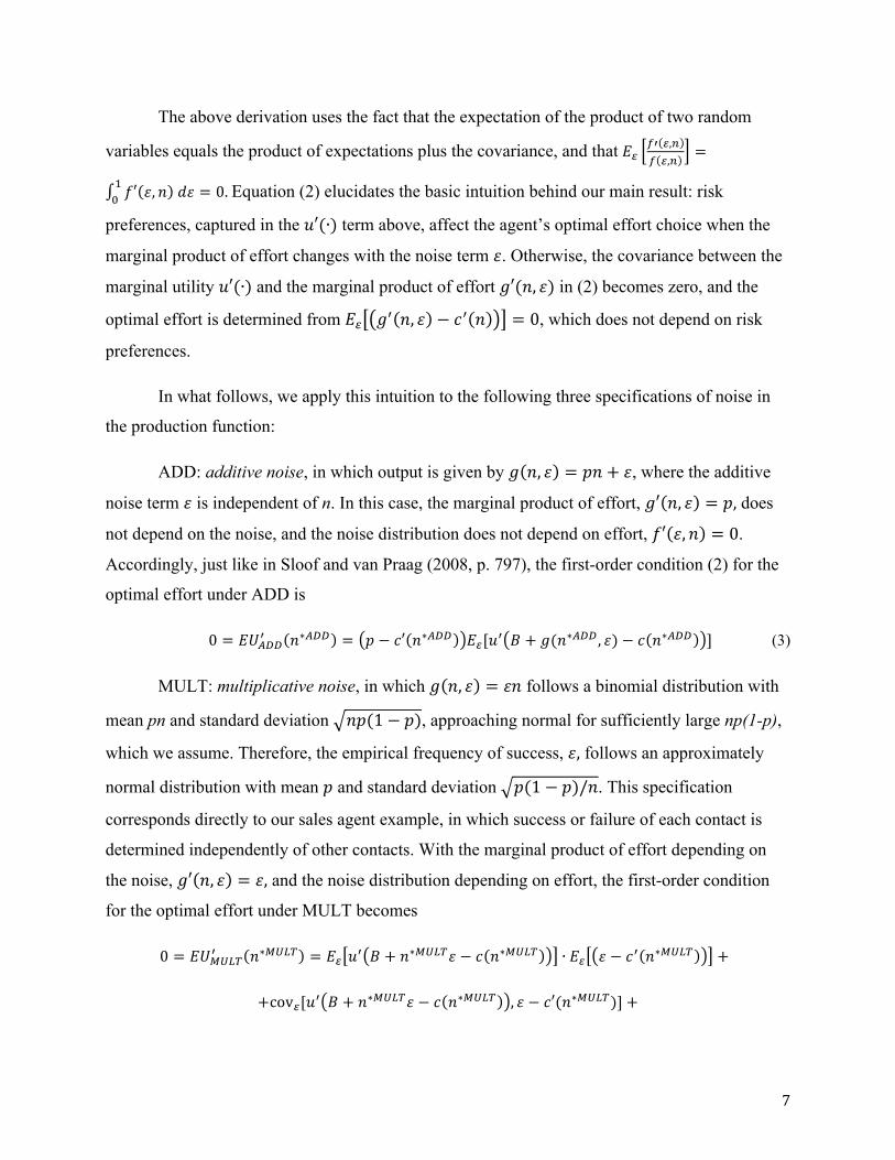
The above derivation uses the fact that the expectation of the product of two random
variables equals the product of expectations plus the covariance, and that %+A: +,$
A +,$=
4′ 1, ( 51<
== 0.Equation (2) elucidates the basic intuition behind our main result: risk
preferences, captured in the ,′(∙) term above, affect the agent’s optimal effort choice when the
marginal product of effort changes with the noise term 1. Otherwise, the covariance between the
marginal utility ,′(∙) and the marginal product of effort /′((, 1) in (2) becomes zero, and the
optimal effort is determined from %+ /: (, 1 − 3: ( = 0, which does not depend on risk
preferences.
In what follows, we apply this intuition to the following three specifications of noise in
the production function:
ADD: additive noise, in which output is given by / (, 1 = D( + 1, where the additive
noise term 1 is independent of n. In this case, the marginal product of effort, /′ (, 1 = D, does
not depend on the noise, and the noise distribution does not depend on effort, 4′ 1, ( = 0.
Accordingly, just like in Sloof and van Praag (2008, p. 797), the first-order condition (2) for the
optimal effort under ADD is
0 = %&EFF:
(∗EFF = D − 3′ (∗EFF %+[,: - + /((∗EFF, 1) − 3 (∗EFF ] (3)
MULT: multiplicative noise, in which / (, 1 = 1( follows a binomial distribution with
mean pn and standard deviation (D(1 − D), approaching normal for sufficiently large np(1-p),
which we assume. Therefore, the empirical frequency of success, 1, follows an approximately
normal distribution with mean D and standard deviation D(1 − D)/(. This specification
corresponds directly to our sales agent example, in which success or failure of each contact is
determined independently of other contacts. With the marginal product of effort depending on
the noise, /′ (, 1 = 1, and the noise distribution depending on effort, the first-order condition
for the optimal effort under MULT becomes
0 = %&JKLM:
(∗JKLM = %+ ,: - + (∗JKLM1 − 3 (∗JKLM ∙ %+ 1 − 3: (∗JKLM +
+cov+[,: - + (∗JKLM1 − 3 (∗JKLM , 1 − 3′((∗JKLM)] +

8
+cov+ , - + (∗JKLM1 − 3 (∗JKLM ,4′ 1, (∗JKLM
4 1, (∗JKLM,
Noting that A: +,$A +,$
=<
N$−
(+OP)Q
NP(<OP)for the normal distribution of 1 under MULT, (4) can be
simplified by replacing the functions ,: . and , . in the covariance terms with their second-
order Taylor approximations around 1 = D, which gives6
0 = %&JKLM:
(∗JKLM = %+ ,: - + (∗JKLM1 − 3 (∗JKLM ∙ %+ 1 − 3: (∗JKLM +
+<
N∙ cov+[,
: - + (∗JKLM1 − 3 (∗JKLM , 1 − 3′((∗JKLM)]. (4a)
Alternatively, recalling equation (2) and using the identity cov+[,: - + (∗JKLM1 − 3 (∗JKLM , 1 −
3′((∗JKLM)] = ,: - + /((∗JKLM, 1) − 3 (∗JKLM 1 − D 4 1, (∗JKLM 51<
=, the same first-order
condition can be rewritten as
0 = %&JKLM:
(∗JKLM = ,: - + /((∗JKLM, 1) − 3 (∗JKLM+RP
N− 3′ (∗JKLM 4 1, (∗JKLM 51
<
=.
(4b)
AON: all or nothing, in which / (, 1 = 1( as before, but now 1 = 1 with probability D
and 0 otherwise. In this specification, the agent is facing progressively more noise than in MULT
because the standard deviation of 1 is larger, D(1 − D) rather than D(1 − D)/(. In terms of
the sales agent example, this specification means that all ( contacts that the agent makes will
simultaneously succeed with probability D and fail with probability 1 − D. As with MULT, the
marginal product of effort under AON depends on the noise; however, the noise distribution is
not affected by effort. Accordingly, the first-order condition for optimal effort under AON is
0 = %&EST:
(∗EST = D,: - + (∗EST − 3 (∗EST 1 − 3: (∗EST − 1 − (5)
6Asecond-orderTaylorseriesexpansionof,: - + (1 − 3(() at1 = Dgives,: - + (1 − 3(() ≈
,: - + (D − 3(() + ,:: - + (D − 3(() ∙ ( ∙ (1 − D) +<
N,::: - + (D − 3(() ∙ (N ∙ (1 − D)N,sothat
V ≡ cov+[,: - + (1 − 3 ( , 1 − 3′(()] = ,:: - + (D − 3(() ∙ ( ∙ var(1 − D) = ,:: - + (D − 3(() (1 − D)D.
Thesameprocedurefor, - + (1 − 3(() renders- ≡ cov+ , - + (1 − 3(() ,<
N$−
(+OP)Q
NP(<OP)= −
<
NP(<OP)∙
<
N,:: - + (D − 3(() ∙ (N ∙ var(1 − D)N = −
<
NP(<OP)∙<
N,:: - + (D − 3(() ∙ (N ∙ 2 var(1 − D) N = −
<
N∙ V.Hence,
V + - =<
N∙ V.
9
D ,: - − 3 (∗EST 3: (∗EST .
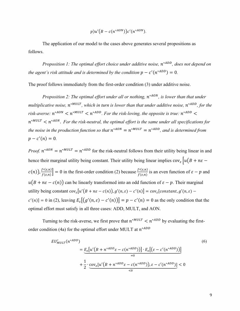
The application of our model to the cases above generates several propositions as
follows.
Proposition 1: The optimal effort choice under additive noise, (∗EFF, does not depend on
the agent’s risk attitude and is determined by the condition D − 3: (∗EFF = 0.
The proof follows immediately from the first-order condition (3) under additive noise.
Proposition 2: The optimal effort under all or nothing, (∗EST, is lower than that under
multiplicative noise, (∗JKLM, which in turn is lower than that under additive noise, (∗EFF, for the
risk-averse: (∗EST < (∗JKLM < (∗EFF. For the risk-loving, the opposite is true: (∗EFF <
(∗JKLM < (∗EST. For the risk-neutral, the optimal effort is the same under all specifications for
the noise in the production function so that (∗EST = (∗JKLM = (∗EFF, and is determined from
D − 3: ( = 0.
Proof. (∗EST = (∗JKLM = (∗EFF for the risk-neutral follows from their utility being linear in and
hence their marginal utility being constant. Their utility being linear implies cov+ , - + (1 −
3 ( ,A: +,$
A +,$= 0 in the first-order condition (2) because A: +,$
A +,$ is an even function of 1 − D and
, - + (1 − 3 ( can be linearly transformed into an odd function of 1 − D. Their marginal
utility being constant cov+ ,: - + (1 − 3 ( , /′((, 1) − 3: ( = cov+ 3[(\]^(], /′((, 1) −
3: ( = 0 in (2), leaving %+ /: (, 1 − 3: ( = D − 3: ( = 0 as the only condition that the
optimal effort must satisfy in all three cases: ADD, MULT, and AON.
Turning to the risk-averse, we first prove that (∗JKLM < (∗EFF by evaluating the first-
order condition (4a) for the optimal effort under MULT at (∗EFF
%&JKLM:
(∗EFF
= %+ ,: - + (∗EFF1 − 3 (∗EFF ∙ %+ 1 − 3: (∗EFF
_=
+1
2∙ cov+[,
: - + (∗EFF1 − 3 (∗EFF , 1 − 3′((∗EFF)]
`=
< 0
(6)

10
The covariance term in (6) is negative because, for the risk-averse, the marginal utility decreases
with 1 whereas the marginal product of effort, /: (, 1 = 1, increases with 1. Because the sign of
the first-order condition (6) is negative, (∗JKLM, which brings (6) to zero, must be less than
(∗EFF.
To prove that (∗EST < (∗JKLM for the risk-averse, we introduce an expression
%&JKLM:
( = ,: - + /((, 1) − 3 ( 1 − 3′ ( 4 1, ( 51<
=< %&JKLM
:( , 7
evaluate it at (∗EST and compare it with %&EST:(∗EST in (5). After some rearrangement of the
terms, the difference between %&JKLM:(∗EST and %&EST:
(∗EST becomes
%&JKLM:
(∗EST − %&EST:
(∗EST = (1 − 3: (∗EST )a + 3′((∗EST)b, (7)
where a = ,: - + (∗EST1 − 3 (∗EST 14 1, (∗EST 51<
=− D,′(- + (∗EST − 3 (∗EST ) and
b = (1 − D),′(- − 3((∗EST)) − ,: - + (∗EST1 − 3 (∗EST 1 − 1 4 1, (∗EST 51<
=. By
concavity of the utility function for the risk averse,
,: - + ( − 3 ( < ,: - + (1 − 3 ( 4 1, ( 51 < ,′(- − 3 ( )
<
=
(8)
for any (.The inequalities in (8) imply a > 0, since %+(1) = D, and b > 0, since %+(1 − 1) =
1 − D. Therefore, %&JKLM:(∗EST > %&JKLM
:(∗EST > %&EST
:(∗EST = 0 for the risk-averse,
implying (∗EST < (∗JKLM.
For the risk-loving, whose utility function is convex, %&JKLM:( > %&JKLM
:( and the
inequalities in (8) reverse, implying (∗EST > (∗JKLM. The statement (∗JKLM > (∗EFF for the
risk-loving follows from (6) because their marginal utility increases with 1.
Proposition 3: The optimal effort levels under multiplicative noise and all or nothing
both decrease with risk aversion. 7Theintegrandin%&d&ef
′( isnegativewhilethatin%&d&ef′
( ispositiveontheinterval23′(() − D < 1 <
3′((),whichisnonemptybecause3′(() < Dfortherisk-averse.Outsidethisinterval,bothintegrandshavethesamesign.Hence,%&d&ef
′( < %&d&ef
′( .

11
Proof. Pratt's (1964) Theorem 1 states that if an agent with a utility function ,<(g) has greater
risk aversion than another agent with a utility function ,N(g) for all g,
,< 5 − ,<(3)
,< h − ,<(^)<,N 5 − ,N(3)
,N h − ,N(^)
for all ^ < h ≤ 3 < 5. In particular, jk:(l)jk:(m)
<jQ:(l)
jQ:(m) for all n < g. The above result applied to the
first-order condition under AON,
0 = %&EST:
(∗EST
= ,: - − 3 (∗EST D 1 − 3: (∗EST,: - + (∗EST − 3 (∗EST
,: - − 3 (∗EST
− 1 − D 3: (∗EST ,
implies the optimal effort (∗EST will go down as increasing risk aversion reduces the ratio
jo pR$∗qrsOt $∗qrs
jo pOt $∗qrs.
Turning to multiplicative noise, rewrite the first-order condition (4b) as
0
= ,: - + 1(∗JKLM − 3 (∗JKLM1 + D
2− 3′ (∗JKLM 4 1, (∗JKLM 51
Nto($∗uvwx)OP
=
`=
+ ,: - + 1(∗JKLM − 3 (∗JKLM1 + D
2− 3′ (∗JKLM 4 1, (∗JKLM 51
<
Nto($∗uvwx)OP
y=
(9)
Pratt's (1964) theorem means that as risk aversion increases, the marginal utility in the positive
part of (9) will decrease relative to the marginal utility in the negative part. Therefore, the
optimal effort (∗JKLM will decrease with risk aversion to restore the equality in (9).
Proposition 4: The difference between optimal effort levels under MULT and AON
increases with risk aversion.

12
Proof. The proof follows from equation (7) that specifies the difference between the first-order
conditions for the optimal effort under MULT and AON evaluated at (∗EST:
%&JKLM:
(∗EST − %&EST:
(∗EST =
(1 − 3: (∗EST )( ,: - + (∗EST1 − 3 (∗EST 14 1, (∗EST 51 − D,′(- + (∗EST<
=
− 3 (∗EST ))
+3′((∗EST)( 1 − D ,: - − 3 (∗EST
− ,: - + (∗EST1 − 3 (∗EST 1 − 1 4 1, (∗EST 51)
<
=
By Pratt’s (1964) theorem, the ratios jo pR$∗qrs+Ot $∗qrs
j:(pR$∗qrsOt $∗qrs ) and
jo pOt $∗qrs
j:(pR$∗qrsOt $∗qrs ) will
increase with risk aversion for all 1 ∈ [0,1]. Hence, %&JKLM:(∗EST − %&EST
:(∗EST will
increase with risk aversion, and so will the difference between (∗JKLM and(∗EST.
Proposition 5: Holding the costs of effort the same across agents, the variance of
individual effort choices increases from ADD to MULT to AON: {^| (∗EST > {^| (∗JKLM >
{^| (∗EFF = 0.
Proof. {^| (∗EFF = 0 by Proposition 1 that states that every agent’s effort choice is determined
by D − 3: (∗EFF = 0 and is independent of risk preferences. {^| (∗JKLM > {^| (∗EFF
because under MULT, unlike ADD, effort varies with risk aversion. {^| (∗EST >
{^| (∗JKLM because Proposition 4 implies a greater variation of effort level with risk aversion
under AON and hence a greater dispersion of individual effort choices.
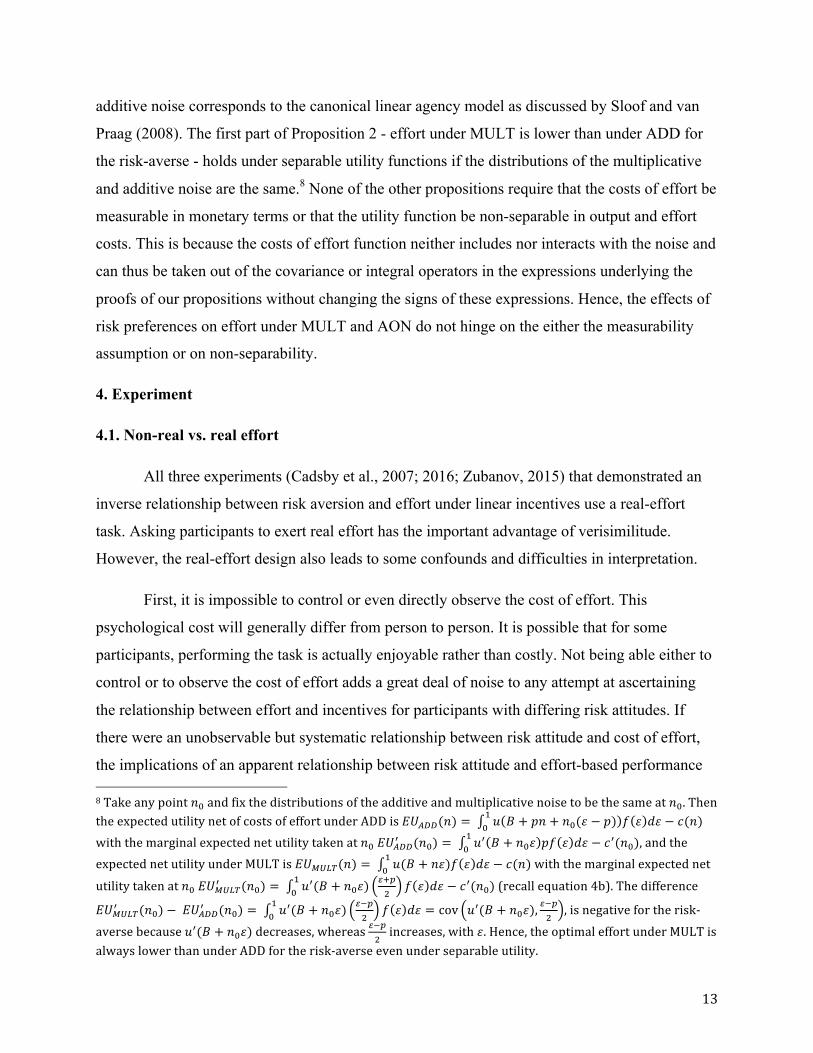
Remark: How dependent is our theory on the assumption that effort is measurable in
monetary terms so that utility is non-separable in output and costs of effort, and can be written as
u(B + g(n,ε) – c(n))? Proposition 1 - effort under ADD being independent of risk preferences -
clearly requires this assumption because otherwise marginal utility, and hence risk
considerations, would be in the first-order condition for effort. In our experiment, where “effort”
and rewards are both denominated in monetary units, this non-separable utility function is
appropriate. This assumption coupled with the assumption of a linear compensation contract and
13
additive noise corresponds to the canonical linear agency model as discussed by Sloof and van
Praag (2008). The first part of Proposition 2 - effort under MULT is lower than under ADD for
the risk-averse - holds under separable utility functions if the distributions of the multiplicative
and additive noise are the same.8 None of the other propositions require that the costs of effort be
measurable in monetary terms or that the utility function be non-separable in output and effort
costs. This is because the costs of effort function neither includes nor interacts with the noise and
can thus be taken out of the covariance or integral operators in the expressions underlying the
proofs of our propositions without changing the signs of these expressions. Hence, the effects of
risk preferences on effort under MULT and AON do not hinge on the either the measurability
assumption or on non-separability.
4. Experiment
4.1. Non-real vs. real effort
All three experiments (Cadsby et al., 2007; 2016; Zubanov, 2015) that demonstrated an
inverse relationship between risk aversion and effort under linear incentives use a real-effort
task. Asking participants to exert real effort has the important advantage of verisimilitude.
However, the real-effort design also leads to some confounds and difficulties in interpretation.
First, it is impossible to control or even directly observe the cost of effort. This
psychological cost will generally differ from person to person. It is possible that for some
participants, performing the task is actually enjoyable rather than costly. Not being able either to
control or to observe the cost of effort adds a great deal of noise to any attempt at ascertaining
the relationship between effort and incentives for participants with differing risk attitudes. If
there were an unobservable but systematic relationship between risk attitude and cost of effort,
the implications of an apparent relationship between risk attitude and effort-based performance 8Takeanypoint(=andfixthedistributionsoftheadditiveandmultiplicativenoisetobethesameat(=.ThentheexpectedutilitynetofcostsofeffortunderADDis%&EFF(() = , - + D( + (=(1 − D) 4 1 51
<
=− 3(()
withthemarginalexpectednetutilitytakenat(=%&EFF:((=) = ,: - + (=1 D4 1 51
<
=− 3:((=),andthe
expectednetutilityunderMULTis%&JKLM(() = ,(- + (1)4 1 51<
=− 3(()withthemarginalexpectednet
utilitytakenat(=%&JKLM:((=) = ,:(- + (=1)
+RP
N4 1 51
<
=− 3:((=)(recallequation4b).Thedifference
%&JKLM:
((=) − %&EFF:
((=) = ,:(- + (=1)+OP
N4 1 51 = cov ,:(- + (=1),
+OP
N
<
=,isnegativefortherisk-
aversebecause,:(- + (=1)decreases,whereas+OP
Nincreases,with1.Hence,theoptimaleffortunderMULTis
alwayslowerthanunderADDfortherisk-averseevenunderseparableutility.

14
could be misinterpreted.
Second, in real-effort experiments, we can generally observe performance, which is the
result of effort. However, it is more difficult to measure effort accurately. For example, while the
number of attempts at a task can be measured and used to represent effort, it is often unclear how
focused and serious a participant’s attempts actually were. Focus and seriousness, while clearly
an aspect of effort, are thus not captured by simple tallies of the number of attempts at a task.
Using performance as a proxy for effort may be problematic also because the relationship
between effort and performance may itself be affected by a participant’s attitude toward financial
risk.
Finally, there is an element of anxiety that may affect observed performance under
incentive pay. When a participant is paid a fixed salary, he or she does not have to worry about
financial uncertainty since the payoff of each participant is predetermined and independent of
performance. However, under a pay-for-performance scheme, financial uncertainty becomes a
potentially important concern because pay is now uncertain and contingent on performance,
which is a product of effort and the probability of success. A more risk-averse participant is by
definition a person who dislikes financial uncertainty. Such a person may therefore feel
uncomfortable in the financially uncertain pay-for-performance environment. This discomfort
may translate into choking under pressure. Despite his or her best efforts, such a person may
choke and perform poorly (Baumeister, 1984; Baumeister and Shower, 1986; Cadsby et al.,
2007; 2016; Ariely et al., 2009). In contrast, a risk-tolerant person might thrive in such an
environment. Thus, in a real-effort experiment, it is very difficult to identify whether an observed
inverse relationship between risk aversion and performance responsiveness to incentives is due
to the hypothesized inverse relationship between risk aversion and effort, to a relationship
between risk aversion and choking under pressure, or to both.
In order to avoid these confounds and focus on the proposed relationship between risk
attitude and effort, we perform a laboratory experiment that eschews real effort in favor of a
menu-based effort-selection design (e.g., Bull, Schotter, and Weigelt, 1987; Fehr, Kirchsteiger,
and Riedl, 1993). The menu specifies the same cost-of-effort function for all participants,
thereby avoiding the problems that arise when this cost is not transparent to the researcher. Since
participants select costly effort without having to actually perform, their effort choices are

15
directly observable and not confounded with potential choking. The results of the experiment
will shed light on the relationship between risk aversion and the performance response to
incentives observed in the cited real-effort experiments. If the hypothesized inverse relationship
between risk-aversion and effort is empirically corroborated, such a relationship likely underlies
at least in part the relationship between risk aversion and performance observed in the real-effort
environment. If in contrast no such relationship is found in our menu-based effort-selection
experiment, it is likely that the observed relationship in the real-effort context was due to
choking under pressure or an unobserved relationship between individual risk attitudes and the
cost of effort.
4.2 Experimental procedures
The experiment was run at Zhejiang University in Hangzhou, China. Participants were
recruited by posting an announcement on an electronic university bulletin board. A total of 180
undergraduate and graduate students from various majors participated in the study. There were
64 males and 116 females with an average age of 21.90 years. The experiment was programmed
and conducted using z-Tree software (Fischbacher, 2007). Each experimental session lasted
about an hour, and the average earnings were 34.2 RMB for each participant inclusive of a 5
RMB show-up fee.9 The average hourly student wage for a part-time job was about 20 RMB at
Zhejiang University at the time of the experiment. Thus, the earnings were salient and attractive
to our participants.
To compare the behavioral responses of each participant in a noiseless control treatment
with their responses to the additive, multiplicative and all-or-nothing treatments, we adopted a
within-person design. Specifically, there was a control treatment with no noise and three
contrasting experimental treatments: additive noise, multiplicative noise, and all-or-nothing
noise. Every participant went through all four treatments in a single session, each of which was
administered in a separate decision period of about 10 minutes. In each period, all participants
were endowed with a sum of 100 Experimental Currency Units (ECUs with 1 ECU = 0.20 RMB)
and their task was to decide how much of that endowment to invest in certificates that would
earn them income in the manner specified for that period. The total cost (TC) of investment was
an increasing function of the number of certificates purchased (n), specifically TC = 0.5n2. Thus, 9 At the time of the experiment, 34.2 RMB was equal to about $5.56.

16
the unit cost (UC) of a certificate also increased with the number of certificates purchased, since
UC = 0.5n. Participants were given not only the cost function itself, but also a table delineating
both the per-unit and total costs corresponding to the number of certificates purchased from 0 to
14.
The rules determining income from investment differed by treatment, and were explained
in the written instructions presented just prior to the period in which the treatment was
administered.10 After reading the instructions for each period, participants answered two
numerical quiz questions to ensure that they understood the instructions correctly. To minimize
various possible confounds that are often associated with within-person experimental designs we
implemented the following procedures. First, to avoid wealth effects, the outcomes of earlier
periods were neither realized nor communicated to participants until all periods were completed.
Second, at the end of the experiment only one of the four decision periods was chosen at random
for payment. Third, to control for possible learning effects, we randomly matched each of the six
possible orderings of the three experimental treatments to one of six separate sessions. The
control treatment was always administered first. There were exactly 30 subjects in each session.
In all four treatments, purchasing ten certificates maximizes the expected monetary payoff. Thus,
a risk-neutral agent would buy ten certificates under all four treatments.
For the Control treatment (denoted CON in what follows), participants were instructed as
follows: “For each certificate you purchase, you will receive 10 ECUs in revenue. Thus, your
total earnings in this period will be calculated as follows: Total Earnings = Endowment + Total
Revenue – Total Cost = 100 + (10 ´ n) – n ´ (0.5 ´ n), where n = the number of certificates
purchased.”
For the Additive Noise treatment (denoted ADD), participants were told: “For each
certificate you purchase, you will receive 10 ECUs in revenue in this period. Thus, your
provisional earnings in this period will be calculated as follows: Provisional Total Earnings =
Endowment + Total Revenue – Total Cost = 100 + (10 ´ n) – n ´ (0.5 ´ n), where n = the
number of certificates purchased. A random process will then determine whether your
provisional earnings will be 1) reduced by 31.6 ECUs, or 2) increased by 31.6 ECUs, with both
10 All instructions used are included in the supplementary material.

17
outcomes having equal probability. Think of the random process as the outcome of a fair coin
toss for which your Final Total Earnings equal your Provisional Earnings – 31.6 ECUs if the
outcome is a head and your Final Total Earnings equal your Provisional Earnings + 31.6 ECUs if
the outcome is a tail.” The additive noise value of 31.6 ECUs was selected so that the variance of
the additive noise process would equal the variance of the multiplicative noise process at n = 10,
the optimal number of certificates for a risk-neutral agent maximizing his/her expected payoff in
the multiplicative noise treatment.
For the Multiplicative Noise treatment (denoted MULT), participants were informed:
“For each certificate you purchase, you will receive either 20 or 0 ECUs in revenue with equal
probability in this period. Think of the revenue from each certificate as the outcome of a fair coin
toss for which the revenue will be 20 ECUs if the outcome is a head, and 0 ECUs if the outcome
is a tail. Note that the revenue outcome for each individual certificate does not in any way
depend on the outcome for any other certificate. This means that whether you receive 20 or 0
ECUs for one of your certificates has no bearing on whether you will receive 20 or 0 ECUs for
any of the other certificates you purchase. Suppose that you purchase n certificates. Of those,
suppose it turns out that you earn 20 ECUs for s certificates and 0 ECUs for the remainder. Then
your earnings will be calculated as follows: Total Earnings = Endowment + Total Revenue –
Total Cost = 100 + (20 ´ s) – n ´ (0.5 ´ n).”
For the All-or-Nothing treatment (denoted AON), we told the participants: “For all the
certificates you purchase, you will receive either 20 or 0 ECUs per certificate in revenue with
equal probability in this period. Think of the revenue as the outcome of a fair coin toss for which
you will receive 20 ECUs times the number of certificates purchased as revenue if it is a head,
and 0 ECUs if it is a tail. Suppose that you purchase n certificates. Then your earnings will be
calculated as follows: Total Earnings = Endowment + Total Revenue – Total Cost = 100 + [(20 ´
n) OR 0 with equal probability] – n ´ (0.5 ´ n).”
At the end of the experiment, we collected demographic information such as gender, age
and study major from all participants. In addition, we asked participants to respond to the
following question: “How do you see yourself: are you generally a person who is fully prepared
to take risks or do you try to avoid taking risks? Please tick a box on the scale 0 (not at all willing

18
to take risks) to 10 (very willing to take risks)”. The response to this question has been used as a
measure of risk aversion (Dohmen et al., 2011; Nosic and Weber, 2010), and has been found to
correlate reliably with behavior involving risk in real situations. We chose this attitudinal
measure over a behavioral elicitation of risk because the experimental treatments themselves
elicit behavior toward different forms of risk.
5. Results
Table 1 reports descriptive statistics by treatment separately for each of the six ordering
sequences, and in aggregate. It also reports analogous results for responses to the question
concerning willingness to take risks. In the last column of Table 1, F tests of equality of means
indicate that neither the average number of certificates purchased in a given treatment nor the
mean participant-reported willingness to take risks varies significantly by the ordering of the
treatments. Non-parametric Kruskal-Wallis tests yield qualitatively identical results.11 We
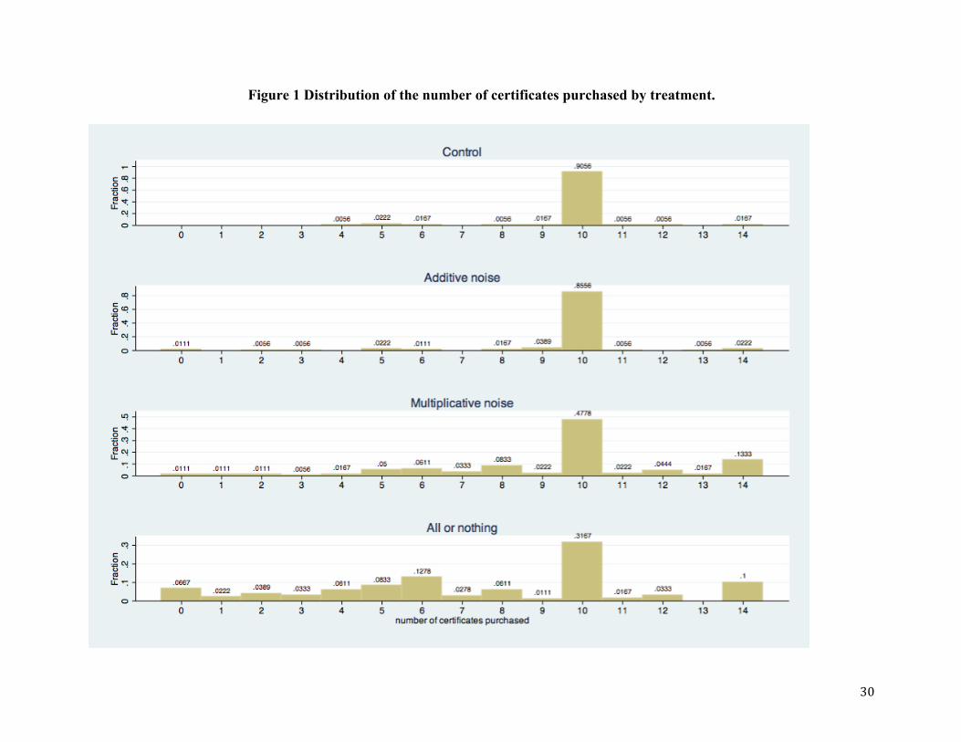
therefore pool the data from the different sessions for analysis. Figure 1 displays the distribution
of the number of certificates purchased by treatment. We focus first on the CON treatment for
which the profit-maximizing choice is to purchase 10 certificates regardless of risk preferences.
It is reassuring that n = 10 was chosen by 163 out of 180 participants, 90.6% of the total. The
mean number of certificates purchased by all 180 participants was equal to 9.844, which a t-test
reveals to be not significantly different from 10. We now proceed to discuss the rest of the
results, numbered to correspond with the theoretical propositions.
[Table 1 here.]
[Figure 1 here.]
Result 1: The number of certificates purchased (effort) under ADD is independent of individual
risk attitudes and is close to 10, which maximizes both the expected monetary payoff and
expected utility.
154 participants, representing 85.6% of the total, purchased ten certificates under ADD.
A t-test reveals that the mean number of 9.689 certificates purchased under ADD does not differ
significantly from 10. The first two columns of Table 2 report regression results for the ADD 11 We also performed Kolmogorov-Smirnov tests on each pair of sequences. In no case could we reject the null hypothesis that the pair of sequences comes from the same underlying distribution.

19
treatment. Our focal explanatory variable is risk aversion, measured by reverse coding
participant responses to our question about willingness to take risks (WTR); that is, higher values
of the "Risk Aversion" variable indicate lower WTR. In column (1), risk aversion is the sole
explanatory variable. In column (2), to check the robustness of our results, we add age, gender,
major and treatment sequence as controls. Age is entered as the reported age of the participant,
gender is specified as a dummy variable, a series of four dummy variables are used to indicate
five broad major categories (biology and medical, arts, science, social science, and other majors)
and five dummies are used for the different treatment sequences. In neither regression is risk
aversion materially related to the number of certificates purchased. None of the controls matter
either.
[Table 2 here.]
Result 2: Of the 163 participants who purchase 10 certificates under CON as predicted, 117
(71.8%) exhibit behavior consistent with our model. Specifically, 30 (18.4%) exhibit consistent
risk-neutral behavior, 65 (39.9%) exhibit consistent risk-averse behaviour, and 22 (13.5%)
exhibit consistent risk-loving behaviour in accordance with Propositions 1 and 2.
Proposition 2 was derived using a continuous function for exertion of effort. In the
experiment, effort was represented by a discrete choice variable: the integer number of
certificates purchased. The model predictions, adapted for the discrete nature of the choices
made by the participants in our laboratory environment are as follows: A risk-neutral participant
will maximize expected earnings by purchasing 10 certificates regardless of treatment, i.e. under
ADD, MULT, and AON. Thus, risk-neutrality implies n*AON = n*MULT = n*ADD = 10. A slightly
risk-averse or slightly risk-loving participant might make identical choices because it is not
permitted to purchase fractional numbers of certificates. For convenience, we categorize all
participants exhibiting such behavior as risk-neutral. For a risk-averse participant, n*AON ≤
n*MULT ≤ n*ADD = 10. For a sufficiently risk-averse participant, at least one of these inequalities
will be strict, and for convenience we require this to categorize a participant as risk-averse.
Analogously, for a risk-loving participant, n*AON ≥ n*MULT ≥ n*ADD = 10 with at least one strict
inequality required to be classified as risk-loving under our categorization. Of those behaving in
accordance with the predictions of our model, it is not surprising to find the majority of
participants exhibit risk-averse behaviour, consistent with many other studies (e.g., Binswanger,

20
1980; Holt and Laury, 2002).
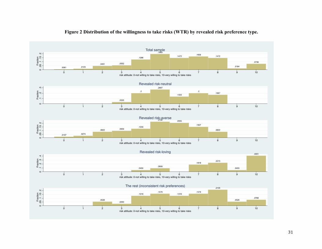
The distributions of the willingness-to-take-risks (WTR) scores differ by revealed risk
preference type. Participants exhibiting revealed risk aversion/risk loving behaviour have
lower/higher average WTR scores than risk-neutral ones. The revealed risk preference types are
correlated, albeit imperfectly, to the reported WTR scores. Figure 2 shows the distributions of
the WTR score by revealed risk preference type. Compared to the entire sample, the WTR
distribution for the risk-neutral is truncated at both tails. Thus, there are no participants claiming
to be extremely risk-loving or risk-averse among the revealed risk-neutral. There is an overall
shift to the left in the WTR distribution for the risk-averse who tend to claim lower WTR, and to
the right for the risk-loving who correspondingly tend to claim a greater willingness to take risks.
The Kolmogorov-Smirnov test for equality of two distributions rejects the hypothesis that WTR
distributions of the risk-averse and risk-loving are the same at p < 0.001. The same test applied
to compare the WTR distributions for risk-neutral and risk-averse, and for risk-neutral and risk-
loving, gives p-values of 0.314 and 0.001 respectively. The mean WTR significantly differs by
type: 5.77 for risk-neutral, 4.96 for risk-averse, and 8.23 for risk-loving, while the equal mean
test yields F = 25.7 with p < 0.001.
[Figure 2 here.]
Result 3: The number of certificates purchased (= our experimental effort) under both MULT
and AON decreases with risk aversion.
The third and fourth columns of Table 2 report regression results for the MULT
treatment. In column (3), risk aversion, again measured by reverse coding the responses to our
WTR question is the sole explanatory variable. In column (4), to check the robustness of our
results, we add age, gender, major and treatment sequence as controls. In both cases, the
coefficient on risk aversion is negative and significant at the one percent level as predicted by
Proposition 3. None of the controls is significant.
The fifth and sixth columns of Table 2 report analogous regression results for the AON
treatment. Once again, the coefficient on risk aversion is negative and significant at the one
percent level both with and without controls. The gender control is significant at the 5% level,

21
indicating that males on average purchase significantly more certificates than females,
controlling for risk aversion as measured by responses to the WTR question.
Result 4: The difference between the number of certificates purchased under MULT and the
number purchased under AON increases with risk aversion.
The seventh and eighth columns of Table 2 report regression results using MULT−AOM
as the dependent variable with and without controls respectively. In both cases, this difference
increases with risk aversion, which is significant at the 1% level. Reflecting the impact of gender
on certificate purchases in the AOM treatment, this difference is significantly lower at the 5%
level for males than for females.
Result 5: The variance of the numbers of certificates purchased in the AON treatment is
significantly greater than the variance in the MULT treatment, and the variance in the MULT
treatment is significantly greater than the variance in the ADD treatment as predicted. However,
the variance in the ADD treatment is 1.705 > 0 contrary to Proposition 5.
The variances for the number of certificates purchased under each treatment are presented
in Table 1. A two-sample variance-comparison test indicates that the variance of 3.913 in the
AON treatment is significantly different from the lower variance of 2.955 in the MULT
treatment (p < 0.001). Moreover, the variance in the MULT treatment is significantly different
from the lower variance of 1.705 in the ADD treatment (p < 0.001). Levene’s robust test statistic
leads to identical conclusions. The variance in the ADD treatment is not equal to zero as
predicted by Proposition 5 because of the 26 out of 180 participants who did not purchase 10
certificates as predicted by Proposition 1.
6. Discussion and conclusion
Effort choice under a given pay-for-performance compensation scheme may be affected
by the way in which financial uncertainty or risk associated with this scheme interacts with
effort. We develop a model to illustrate how this can occur, and run an experiment to investigate
whether people make effort choices consistent with our model. Our experiment was designed to
focus on how risk attitude affects selected effort levels under different risk specifications. We
show that if financial uncertainty increases with the amount of effort exerted, as in the

22
multiplicative noise and all-or-nothing treatments, risk-averse individuals will exert less effort
and accept a lower expected return to mitigate risk, while risk-loving individuals will exert more
effort, accepting greater risk and a lower expected return in pursuit of the chance of a large
payoff. We also show that when financial uncertainty is not affected by effort, as in the additive
noise treatment, risk preferences do not affect effort choices. We find that 163 out of our 180
participants select the payoff-maximizing level of costly effort from a menu of choices in a no-
noise control treatment. Of those, 71.8% make decisions consistent with the predictions of our
model in all three experimental treatments. Specifically, 39.9% are consistently risk-averse,
13.5% are consistently risk-loving, and 18.4% are consistently risk-neutral. Effort decisions in
the face of multiplicative or all-or-nothing risk, both of which increase with effort, may be
thought of as analogous to the decision of an investor choosing the proportion of wealth to hold
in a safe asset versus a risky portfolio. This is because conservation of costly effort has a safe
and certain return, while exerting more effort produces an increasingly uncertain payoff.
In order to avoid potential confounds in testing experimentally the effect of risk attitude
on effort under different risk specifications, it was important to control the cost of effort, and to
avoid requiring the performance of a task that might be affected by choking under the pressure of
financial uncertainty. This was accomplished by means of a menu-based effort-selection design,
which is complementary to the previous real-effort approaches to studying the impact of risk
attitude on the response to pay-for-performance incentives. The strong corroboration of an
inverse relationship between risk aversion and effort under both multiplicative and all-or-nothing
noise suggests that such a relationship is an important mediating component of the previously
observed inverse relationship between risk aversion and the performance response to incentives
in the real-effort case.
Rooted in the workers’ utility function and the methods firms use to measure and reward
performance, the relationship between risk aversion and effort is likely to be enduring and
important for management practice for two reasons. First, multiplicative noise, under which this
relationship holds, occurs whenever the marginal product of effort is uncertain at the time of
effort choice. Examples of such situations are many and include effort spent on research and
development of new technologies and products, effort spent on marketing campaigns as well as
the sales agent example used to motivate this study.

23
Second, linking our study with the related literature on background risk (Gollier and
Pratt, 1996; Beaud and Willinger, 2015) suggests that additive background risk may amplify the
effect of multiplicative noise on effort. In real world settings, many workers making effort
choices face such background risk. Consider an environment that exposes an employee to both
additive background risk and multiplicative or all-or-nothing risk that increases with his/her
choice of effort level. An increase in additive background risk in the presence of multiplicative
or all-or-nothing risk will increase absolute risk aversion thereby causing the risk vulnerable to
reduce their effort. Similarly, multiplicative or all-or-nothing risk would have a stronger effect
on the effort exerted by the risk vulnerable when they are already experiencing uncontrollable
additive risk.
Since it is the result rather than effort per se that is often rewarded, it is vital that
incentive compensation schemes reflect the link between risk aversion and effort. There are
several practical alternatives to the linear output-based incentives under multiplicative noise
considered in this study. One is to reward effort rather than output, that is, to pay the sales agent
per customer contact rather than per successful transaction. In our example, when the probability
of a deal is independent of effort, paying a risk-averse agent per contact is an improvement over
paying per successful transaction because it removes all risks from the agent's pay. However,
when the probability of a successful outcome does depend on effort, paying per contact will lead
to all effort being spent on making new contacts and none on cultivating existing ones. An
element of pay per successful transaction would therefore be required as part of total
compensation, bringing the negative risk aversion-effort link back to the fore.
Another alternative is to offer convex output-based incentives, whereby the agent's pay
grows faster than his/her output to compensate for the increasing costs of bearing multiplicative
risk. However, such convex incentives may encourage excessive risk taking by less risk-averse
agents, in much the same way as they have done in the hedge fund industry (de Figueiredo et al.,
2013). An alternative to globally convex incentives are locally convex ones, which encourage
extra effort from the risk-averse agents who would otherwise have chosen low effort while not
giving extra incentive for risk taking to the harder-working, less risk-averse agents. A typical
example of locally convex incentives is a target bonus paid on top of the usual earnings once
output reaches the target. Our work helps to understand why such locally convex incentive

24
schemes exist and suggests that their parameters should take account of the performance
measurement technology as well as risk preferences.

25
References:
Ariely, D., Gneezy, U., Loewenstein, G., and Mazar, N. 2009. Large stakes and big mistakes.
Review of Economic Studies, 76(2): 451–469.
Baker, G. P., and Jorgensen, B. 2003. Volatility, noise, and incentives.
http://www.people.hbs.edu/gbaker/oes/papers/Baker_Jorgensen.pdf.
Baumeister, R. F. 1984. Choking under pressure: Self-consciousness and paradoxical effects of
incentives on skillful performance. Journal of Personality and Social Psychology, 46(3):
610–620.
Baumeister, R. F., and Showers, C. J. 1986. A review of paradoxical performance effects:
Choking under pressure in sports and mental tests. European Journal of Social Psychology,
16(4): 361–383.
Beaud, M., Willinger, M. 2015. Are people risk vulnerable? Management Science, 61(3), 624-
636.
Bellemare, C., and Shearer, B. 2010. Sorting, incentives and risk preferences: Evidence from a
field experiment. Economics Letters, 108: 345-348.
Binswanger, H. P. 1980. Attitudes toward risk: Experimental measurement in rural India.
American Journal of Agricultural Economics, 62: 395–407.
Bull, C., Schotter, A., and Weigelt, K. 1987. Tournaments and piece rates: An experimental
study. Journal of Political Economy, 95: 1-33.
Cadsby, C. B., Song, F. and Tapon, F. 2007. Sorting and incentive effects of pay for
performance: An experimental investigation. Academy of Management Journal, 50: 387–405.
Cadsby, C. B., Song, F. and Tapon, F. 2016. The Impact of Risk Aversion and Stress on the
Incentive Effect of Performance Pay. Research in Experimental Economics Vol.19,
Experiments in Organizational Economics, edited by S. Goerg and J. Hammon, series editors
R.M. Isaac and D.A. Norton, Emerald Group Publishing.
de Figueiredo, R., Rawley, E., Shelef, O. 2013. Bad bets: Excessive risk taking, convex
incentives, and performance. Stanford Institute for Economic Policy Research discussion
paper 13-002.
Dohmen, T., Falk, A., Huffman, D., Sunde, U., Schupp, J., and Wagner, G. 2011. Individual risk
attitudes: Measurement, determinants and behavioral consequences. Journal of the European
Economic Association, 9: 522-550.
26
Eeckhoudt, L., Gollier, C., and Schlesinger, H. 1995. The risk-averse (and prudent) newsboy.
Management Science, 41(5), 786-794.
Eckel, C. and Grossman, P. 2002. Sex differences and statistical stereotyping in attitudes towards
financial risk. Evolution and Human Behavior, 23(4), 281-295.
Eckel, C. and Grossman, P. 2008. Forecasting risk attitudes: An experimental study using actual
and forecast gamble choices. Journal of Economic Behavior and Organization, 68(1), 1-7.
Fehr, E., Kirchsteiger, G., and Riedl, A. 1993. Does Fairness Prevent Market Clearing? An
Experimental Investigation. The Quarterly Journal of Economics,108: 437-459.
Fischbacher, U. 2007. z-Tree: Zurich toolbox for ready-made economic experiments.
Experimental Economics, 10: 171-178.
Franke, G., Schlesinger, H., Stapleton, R.C. 2006. Multiplicative background risk. Management
Science, 52(1), 146-153.
Gollier, C., Pratt, J. W. 1996. Risk vulnerability and the tempering effect of background risk.
Econometrica, 64(5), 1109-1123.
Grund, C. and Sliwka, D. 2010. Evidence of performance pay and risk aversion. Economics
Letters, 102: 8-11.
Holt, C. and Laury, S. 2002. Risk Aversion and Incentive Effects. American Economic Review,
92(5): 1644–1655.
Lo, H.-F., Ghosh, M. and Lafontaine, F. 2011. The incentive and selection roles of sales force
compensation contracts. Journal of Marketing Research, 48, 781-798.
Nosic, A. and Weber, M. 2010. How risky do I invest? The role of risk attitudes, risk
perceptions, and overconfidence. Decision Analysis, 7, 282-301.
Pratt, J. 1964. Risk aversion in the small and in the large. Econometrica, 32(1/2), 122 –136.
Prendergast, C. 1999. The provision of incentives in firms. Journal of Economic Literature, 37,
7–63.
Reynaud, A. and Couture, S. 2012. Stability of risk preference measures: Results from a field
experiment on French farmers. Theory and Decision, 73(2), 203-221.
Sharpe, W. F. 1964. Capital asset prices: A theory of market equilibrium under conditions of
risk. Journal of Finance, 19 (3), 425-442.
Sloof, R. and van Praag, C. M. 2008. Performance measurement, expectancy and agency theory:
An experimental study. Journal of Economic Behavior and Organization, 67(3-4): 794–809.

27
Sloof, R. and van Praag, C. M. 2010. The effect of noise in a performance measure on work
motivation: A real effort laboratory experiment. Labour Economics, 17, 751-765.
Tobin, J. 1958. Liquidity preference as behavior towards risk. The Review of Economic Studies,
25, 65-86.
Zubanov, N. 2015. Risk aversion and effort in an incentive pay scheme with multiplicative noise:
Theory and experimental evidence. Evidence-based HRM: A Global Forum for Empirical
Scholarship, 3: 130-144.

28
Table 1 Descriptive Statistics
Overall Means by treatment sequence
Number of certificates purchased (n):
Mean Variance 1 2 3 4 5 6 t tests of equal means
p-value
CON: no noise 9.844 1.157 9.800 9.967 9.655 10.129 9.800 9.700 0.378
ADD: additive noise 9.689 1.705 9.667 9.800 10.000 9.645 9.533 9.500 0.634
MULT: multiplicative noise
9.472 2.955 9.100 9.967 9.379 9.774 9.400 9.200 0.852
AON: all or nothing 7.561 3.913 7.267 8.200 8.103 6.355 7.667 7.833 0.413
Personal assessment of willingness to take risks (r) (0=not willing, 10=very willing)
5.839 2.128 5.333 6.467 5.621 5.290 6.233 6.100 0.156

29
Table 2 Regression Results of Certificates Purchased (Effort) on Risk Aversion and Controls
ADD
(1)
ADD
(2)
MULT
(3)
MULT
(4)
AON
(5)
AON
(6)
MULT - AON
(7)
MULT - AON
(8)
Risk Aversion
-0.030
(0.043)
-0.024
(0.042)
-0.377
(0.115)
-0.424
(0.113)
-0.947
(0.107)
-0.915
(0.115)
-0.568
(0.147)
-0.491
(0.153)
Age -0.131
(0.010)
-0.053
(0.110)
-0.034
(0.132)
-0.019
(0.163)
Male 0.334
(0.229)
0.718
(0.486)
1.645
(0.592)
-0.927
(0.697)
Major no yes no yes no yes no yes
Treatment sequence
no yes no yes no yes no yes
Notes: 180 obs. Robust standard errors are in parentheses. Risk aversion is measured as the willingness to take risks (WTR) recoded so that low values of risk aversion correspond to high values of WTR.
30
Figure 1 Distribution of the number of certificates purchased by treatment.
31
Figure 2 Distribution of the willingness to take risks (WTR) by revealed risk preference type.
.0061 .0123.0491 .0552
.1288
.1963
.1472.1656
.1472
.0184
.0736
0.0
5.1
.15
.2Fr
actio
n
0 1 2 3 4 5 6 7 8 9 10risk attitude: 0-not willing to take risks, 10-very willing to take risks
Total sample
.0333
.2
.2667
.1333
.2.1667
0.1
.2.3
Frac
tion
0 1 2 3 4 5 6 7 8 9 10risk attitude: 0-not willing to take risks, 10-very willing to take risks
Revealed risk-neutral
.0137 .0274
.0822 .0959.1233
.2192 .2055
.1507
.0822
0.0
5.1
.15
.2Fr
actio
n
0 1 2 3 4 5 6 7 8 9 10risk attitude: 0-not willing to take risks, 10-very willing to take risks
Revealed risk-averse
.0455.0909
.1818.2273
.0455
.4091
0.1
.2.3
.4Fr
actio
n
0 1 2 3 4 5 6 7 8 9 10risk attitude: 0-not willing to take risks, 10-very willing to take risks
Revealed risk-loving
.0526.0263
.1316.1579
.1316.1579
.2105
.0526.0789
0.0
5.1
.15
.2Fr
actio
n
0 1 2 3 4 5 6 7 8 9 10risk attitude: 0-not willing to take risks, 10-very willing to take risks
The rest (inconsistent risk preferences)


