
Training Neural Networks

Accelerate innovation by unifying data science, engineering and business
• Founded by the original creators of Apache Spark
• Contributes 75% of the open source code, 10x more than any other company
• Trained 100k+ Spark users on the Databricks platform
VISION
WHO WE ARE
Unified Analytics Platform powered by Apache Spark™PRODUCT

About our speaker
Denny Lee Technical Product Marketing Manager
Former: • Senior Director of Data Sciences Engineering at SAP Concur • Principal Program Manager at Microsoft
• Azure Cosmos DB Engineering Spark and Graph Initiatives • Isotope Incubation Team (currently known as HDInsight) • Bing’s Audience Insights Team • Yahoo!’s 24TB Analysis Services cube

Deep Learning Fundamentals Series
This is a three-part series:
• Introduction to Neural Networks
• Training Neural Networks
• Applying your Convolutional Neural Network
This series will be make use of Keras (TensorFlow backend) but as it is a fundamentals series, we are focusing primarily on the concepts.
Previous Session: Introduction to Neural Networks
• What is Deep Learning?
• What can Deep Learning do for you?
• What are artificial neural networks?
• Let’s start with a perceptron…
• Understanding the effect of activation functions

Current Session: Training Neural Networks
• Tuning training
• Training Algorithms
• Optimization (including Adam)
• Convolutional Neural Networks

Upcoming Session: Applying Neural Networks
• Diving further into CNNs
• CNN Architectures
• Convolutions at Work!

Convolutional Neural Networks
28 x 28 28 x 28 14 x 14
Convolution 32 filters
Convolution 64 filters
Subsampling Stride (2,2)
Feature Extraction Classification
01
89
Fully Connected
Dropout
Dropout

Tuning Training

Hyperparameters• Network • How many layers? • How many neurons in each layer? • What activation functions to use?
• Learning algorithm • What’s the best value of the learning rate? • How quickly decay the learning rate? Momentum? • What type of loss function should I use? • What batch size? • How many iterations is enough?

Overfitting and underfitting

Overfitting and underfitting

Overfitting and underfitting

Hyperparameters: NetworkGenerally, the more layers and the number of units in each layer: • The greater the capacity of the artificial neural network • The risk is overfitting when your goal is to build a generalized model.
From a practical perspective, a good starting point is: • The number of input units equals the dimension of features • The number of output units equals the number of classes (e.g. in the MNIST dataset, there
are 10 possible values represents digits (0…9) hence there are 10 output units • Start with one hidden layer that is 2x the number of input units • A good reference is Andrew Ng’s Coursera Machine Learning course.

Hyperparameters: Activation Functions?• Good starting point: ReLU • Note many neural networks samples: Keras MNIST, TensorFlow CIFAR10 Pruning, etc. • Note that each activation function has its own strengths and weaknesses. A good quote
on activation functions from CS231N summarizes the choice well:
“What neuron type should I use?” Use the ReLU non-linearity, be careful with your learning rates
and possibly monitor the fraction of “dead” units in a network. If this concerns you, give Leaky
ReLU or Maxout a try. Never use sigmoid. Try tanh, but expect it to work worse than ReLU/
Maxout.

Neurons … Activate!
DEMO

HyperparametersLearning algorithm
• What’s the best value of the learning rate?
• How quickly decay the learning rate? Momentum?
• What type of loss function should I use?
• What batch size?
• How many iterations is enough?
Training Algorithms

Cost function
Source: https://bit.ly/2IoAGzL
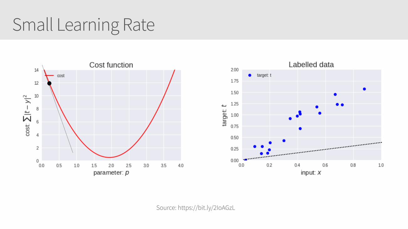
For this linear regression example, to determine the best (slope of the line) for
we can calculate the cost function, such as Mean Square Error, Mean absolute error, Mean bias error, SVM Loss, etc.
For this example, we’ll use sum of squared absolute differences
𝑦 = 𝑥 ⋅ 𝑝
𝑝
𝑐𝑜𝑠𝑡 = ∑ | 𝑡 − 𝑦 |2

Gradient Descent Optimization
Source: https://bit.ly/2IoAGzL

Small Learning Rate
Source: https://bit.ly/2IoAGzL
Small Learning Rate
Source: https://bit.ly/2IoAGzL

Small Learning Rate
Source: https://bit.ly/2IoAGzL

Small Learning Rate
Source: https://bit.ly/2IoAGzL

Simplified Two-Layer ANN
1
1
0.8
0.2
0.7
0.6
0.9
0.1
0.8
0.75
0.69
h1 = 𝜎(1𝑥0.8 + 1𝑥0.6) = 0.80h2 = 𝜎(1𝑥0.2 + 1𝑥0.9) = 0.75h3 = 𝜎(1𝑥0.7 + 1𝑥0.1) = 0.69

Simplified Two-Layer ANN
1
1
0.8
0.2
0.7
0.6
0.9
0.1
0.8
0.75
0.69
0.2
0.8
0.5
0.75
𝑜𝑢𝑡 = 𝜎(0.2𝑥0.8 + 0.8𝑥0.75 + 0.5𝑥0.69)
= 𝜎(1.105)
= 0.75

Backpropagation
Input Hidden Output
0.8
0.2
0.75

Backpropagation
Input Hidden Output
0.85
• Backpropagation: calculate the
gradient of the cost function in a
neural network
• Used by gradient descent optimization
algorithm to adjust weight of neurons
• Also known as backward propagation
of errors as the error is calculated and distributed back through the network of layers
0.10

Sigmoid function (continued)
Output is not zero-centered: During gradient
descent, if all values are positive then during
backpropagation the weights will become all
positive or all negative creating zig zagging
dynamics.
Source: https://bit.ly/2IoAGzL

Learning Rate Callouts
• Too small, it may take too long to get minima
• Too large, it may skip the minima altogether

Optimization

Optimization Overview• After backpropagation, the parameters are updated based on the gradients
calculated
• There are several approaches in this area of active research; we will focus on:
• Stochastic Gradient Descent • Momentum, NAG • Per-parameter adaptive learning rate methods

Stochastic Gradient Descent
• (Batch) Gradient Descent is computed on the full dataset (not efficient for large scale models and datasets).
• Often converges faster because it performs updates more frequently • But due to frequent updates, this may complicate convergence to the exact
minima • For more information, refer to: • Andrew Ng’s 2. Stochastic Gradient (https://goo.gl/bNrJbx) • Types of Optimization Algorithms used in Neural Networks and Ways to
Optimize Gradient Descent (https://goo.gl/tB2e7S)

Gradient Descent Source: https://goo.gl/VUX2ZS

Momentum and NAG
• Obtain faster convergence by helping parameter vector build up velocity • i.e. use the momentum of the gradient to converge faster
• Nesterov Accelerated Gradient (NAG): optimized version of Momentum • Typically works better in practice than Momentum
Source: http://cs231n.github.io/neural-networks-3

Annealing the learning rate
• i.e. slow down the learning rate to prevent it from bouncing around too much
• Referred as the decay parameter (i.e., the learning rate decay over each
update) to reduce kinetic energy
• Note, this is different from rho (i.e. exponentially weighted average or exponentially weighted decay of past gradients) to smooth the descent path trajectory

Per-parameter adaptive learning rate methods• Adaptively tune learning rates at the parameter level
• Popular methods include: • Adaptive Gradient Algorithm (AdaGrad) improves performance on problems with sparse
gradients (e.g. natural language and computer vision problems). • Root Mean Square Propagation (RMSProp) maintains per-parameter learning rates based
on the average of recent magnitudes of the gradients for the weight (e.g. how quickly it is changing). This means the algorithm does well on online and non-stationary problems (e.g. noisy).
• AdaDelta: Per dimension learning rate method for gradient descent with minimal computational overhead, requires no manual tuning, and quite robust

Which Optimizer?
“In practice Adam is currently recommended as the default algorithm to use, and often works slightly better than RMSProp. However, it is often also worth trying SGD+Nesterov Momentum as an alternative..”
Andrej Karpathy, et al, CS231n
Source: https://goo.gl/2da4WY
Comparison of Adam to Other Optimization Algorithms Training a Multilayer Perceptron Taken from Adam: A Method for Stochastic Optimization, 2015.

Optimization on loss surface contours
Adaptive algorithms converge quickly and find the right direction for the parameters.
In comparison, SGD is slow
Momentum-based methods overshoot
Source: http://cs231n.github.io/neural-networks-3/#hyper Image credit: Alec Radford
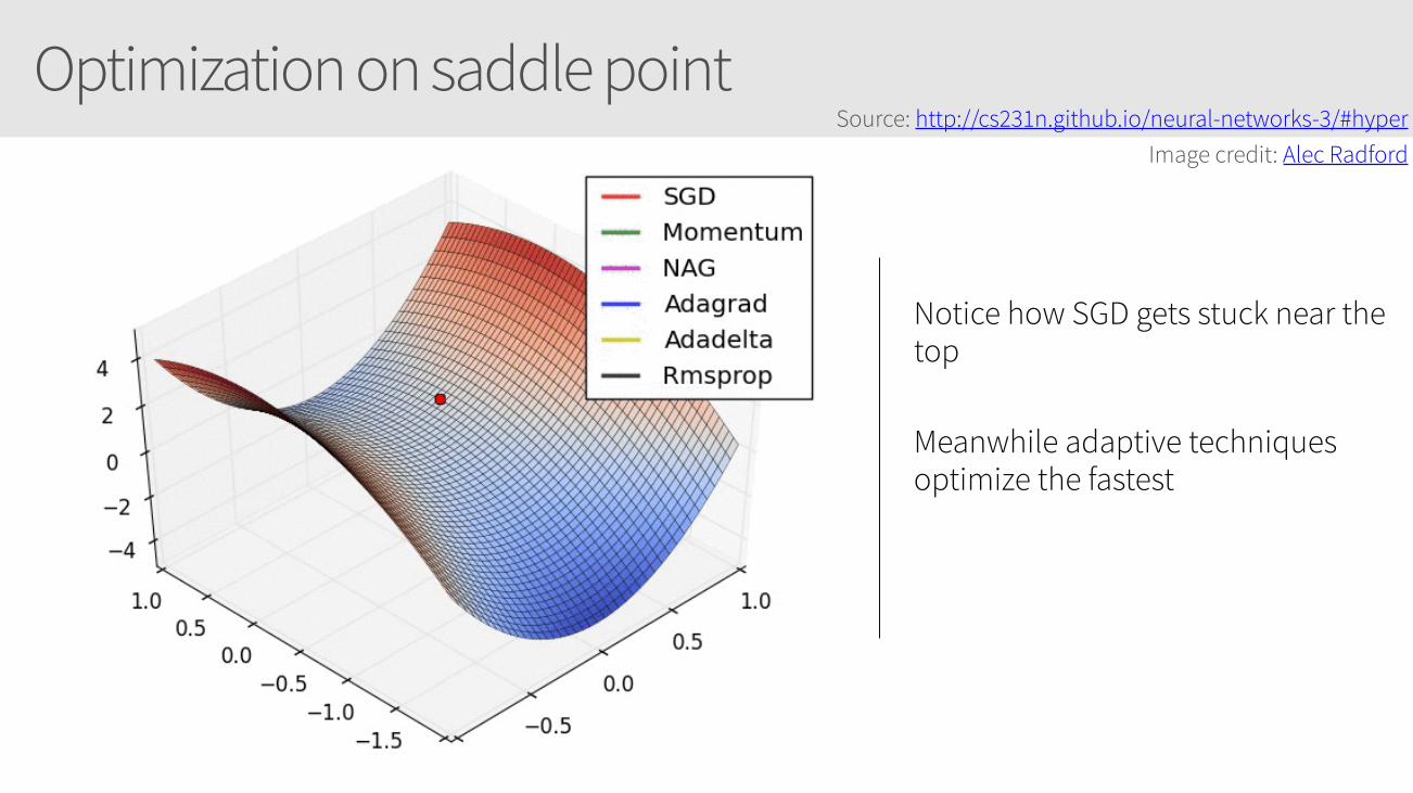
Optimization on saddle point
Notice how SGD gets stuck near the top
Meanwhile adaptive techniques optimize the fastest
Source: http://cs231n.github.io/neural-networks-3/#hyper Image credit: Alec Radford

Good References• Suki Lau's Learning Rate Schedules and Adaptive Learning Rate Methods for
Deep Learning
• CS23n Convolutional Neural Networks for Visual Recognition
• Fundamentals of Deep Learning
• ADADELTA: An Adaptive Learning Rate Method
• Gentle Introduction to the Adam Optimization Algorithm for Deep Learning

Convolutional Networks

Convolutional Neural Networks
• Similar to Artificial Neural Networks but CNNs (or ConvNets) make explicit assumptions that the input are images
• Regular neural networks do not scale well against images • E.g. CIFAR-10 images are 32x32x3 (32 width, 32 height, 3 color channels) =
3072 weights – somewhat manageable • A larger image of 200x200x3 = 120,000 weights
• CNNs have neurons arranged in 3D: width, height, depth. • Neurons in a layer will only be connected to a small region of the layer before
it, i.e. NOT all of the neurons in a fully-connected manner. • Final output layer for CIFAR-10 is 1x1x10 as we will reduce the full image into
a single vector of class scores, arranged along the depth dimension

CNNs / ConvNets
Regular 3-layer neural network
• ConvNet arranges neurons in 3 dimensions • 3D input results in 3D output
Source: https://cs231n.github.io/convolutional-networks/

Convolutional Neural Networks
28 x 28 28 x 28 14 x 14
Convolution 32 filters
Convolution 64 filters
Subsampling Stride (2,2)
Feature Extraction Classification
01
89
Fully Connected
Dropout
Dropout

Convolutional Neural Networks
28 x 28 28 x 28 14 x 14
Convolution 32 filters
Convolution 64 filters
Subsampling Stride (2,2)
Feature Extraction Classification
01
89
Fully Connected
Dropout
Dropout
Input Pixel value of 32x32x3: 32 width, 32 height, 3 color channels (RGB)

Convolutional Neural Networks
28 x 28 28 x 28 14 x 14
Convolution 32 filters
Convolution 64 filters
Subsampling Stride (2,2)
Feature Extraction Classification
01
89
Fully Connected
Dropout
Dropout
Convolutions Compute output of neurons (dot product between their weights) connected to a small local region. If we use 32 filters, then the output is 28x28x32 (using 5x5 filter)

Convolutional Neural Networks
28 x 28 28 x 28 14 x 14
Convolution 32 filters
Convolution 64 filters
Subsampling Stride (2,2)
Feature Extraction Classification
01
89
Fully Connected
Dropout
Dropout
Pooling Perform down sampling operation along spatial dimensions (w, h) resulting in reduced volume, e.g. 14x14x2.

Convolutional Neural Networks
28 x 28 28 x 28 14 x 14
Convolution 32 filters
Convolution 64 filters
Subsampling Stride (2,2)
Feature Extraction Classification
01
89
Fully Connected
Dropout
Dropout
Fully Connected Neurons in a fully connected layer have full connections to all activations in the previous layer, as seen in regular Neural Networks.

https://cs.stanford.edu/people/karpathy/convnetjs/demo/mnist.html
ConvNetJS MNIST Demo

Neurons … Activate!
DEMO
I’d like to thank…

Great References• Andrej Karparthy’s ConvNetJS MNIST Demo
• What is back propagation in neural networks?
• CS231n: Convolutional Neural Networks for Visual Recognition
• Syllabus and Slides | Course Notes | YouTube
• With particular focus on CS231n: Lecture 7: Convolution Neural Networks
• Neural Networks and Deep Learning
• TensorFlow

Great References• Deep Visualization Toolbox
• Back Propagation with TensorFlow
• TensorFrames: Google TensorFlow with Apache Spark
• Integrating deep learning libraries with Apache Spark
• Build, Scale, and Deploy Deep Learning Pipelines with Ease

AttributionTomek Drabas Brooke Wenig Timothee Hunter Cyrielle Simeone

Q&A

What’s next?Applying your Convolutional Neural NetworkOctober 25, 2018 | 10:00 PDThttps://dbricks.co/2O2c4BZ
State Of The Art Deep Learning On Apache Spark™October 31, 2018 | 09:00 PDT
https://dbricks.co/2NqogIp


