
Does Affirmative Action Work?
Evaluating India’s Quota System
Alexander Lee∗
October 15, 2020
Abstract
This paper examines two common critiques of ethnic quota policies in government hiring
and education: that they do not benefit the target group, and that any benefits are unevenly
distributed within the target group. It focuses on the effects of educational and hiring quotas
for Other Backward Class (OBC) castes in India, using difference-in-difference and triple
difference designs that take advantage of the gradual introduction of these quotas. The results
provide little support for these critiques: affirmative action is associated with small increases
in educational attainment and government employment among eligible age cohorts, though
the increases in government employment may be a result of other social and political trends.
These benefits extend even to poorer OBCs (though not the very poorest), and increase the
chances of social contact between uneducated OBCs and government officials.1
∗Department of Political Science, University of Rochester Thanks to Bill Ktai’pi, Jack Paine, Nishith Prakash,and seminar participants at the University of Connecticut, University of California Riverside and the AmericanPolitical Science Association and Southern Political Science Association Annual Meetings for comments on themanuscript, and to Bridgette Wellington, Fred Arnold and K.S. James for assistance in obtaining data.
1Replication materials and code can be found at the Harvard Dataverse, https://doi.org/10.7910/DVN/YWKZHJ,(Lee, 2020)

1 Introduction
Many countries have severe economic inequalities between ethnic groups, often the result of
deep-seated social discrimination or legacies of previous discrimination (Cederman et al., 2010). One
of the most common proposed solutions to such problems is the introduction of quotas or other
preferential practices in educational admissions and government hiring processes. For example, in
the United States African American and Latino/a applicants are granted preferential treatment
in admissions to most universities and in hiring for many government or private sector jobs, while in
India a proportion of places at public universities and jobs in public sector institutions are “reserved”
for members of specific lower caste groups. The efficacy and justice of these policies have been, and
continue to be, fiercely debated (e.g. Sowell, 2005; Kennedy, 2013).
In both the United States and India, critics of affirmative action frequently make empirical claims
about the effects of these polices. First, some claim affirmative action does not fulfill its primary goal
of raising the socioeconomic status of the targeted group due to limited scope or poor “matching” of
recipients to opportunities, leading to high rates of failure and no lasting gain (Sander, 2004). Second,
some claim that any benefits of affirmative action are disproportionately concentrated among the
socio-economic elite of the targeted group (Massey et al., 2006; Galanter, 1984; Sowell, 2005). If this
is correct, quotas might not change the proportion of the disadvantaged group that is disadvantaged,
and might even lead to poor applicants from the advantaged group being disfavored relative to
wealthier ones from the disadvantaged group.
Despite the importance of the question, the purely empirical literature on educational and hiring
preferences is modest in size, particularly relative to the flourishing literature on the effects of electoral
quotas (Jensenius, 2017; Chauchard, 2014; Dunning and Nilekani, 2013; Karekurve-Ramachandra
and Lee, ming), and the effects of quotas on institutional efficiency (Bhavnani and Lee, 2019;
Bertrand et al., 2010). In fact, only the first of these critiques has been the subject of sustained

empirical investigation, much of it challenging the “matching” hypothesis (Howard and Prakash,
2012; Arcidiacono, 2005; Loury and Garman, 1993; Hinrichs, 2012). However, there is virtually no
empirical little work on the distribution of benefits within the target group, or effects outside the
immediate beneficiaries. The institutional effects of quotas are thus somewhat better understood
than their social effects, despite the importance of the social effects in normative debates on the topic.
This project focuses on a particularly controversial instance of affirmative action: the gradual
implementation of hiring quotas for members of the Other Backward Classes (OBC) social category
in India. Some Indian caste groups (jatis) are much poorer than others, whether because of different
traditional occupations, colonial policies, or continuing discrimination against “low” caste groups.
Two categories of groups with very low social status, the Scheduled Castes (SCs) and Scheduled
Tribes (STs) have enjoyed quotas (“reservations”) in university admissions and state and central
government hiring throughout India’s post-independence history. Reservations for OBCs (the low
status groups not sufficiently disadvantaged to be included in the first two categories) were also
instituted in some states during the early and mid 20th century, and in 1994, OBC reservations
were instituted both at the national level and at the state level in all states that had not already
adopted them. The wisdom and scope of OBC reservations were, and are still, extremely politically
important in India (Jaffrelot, 2003; Suryanarayan, 2019).
One reason for the small size of the literature on non-electoral preferences (at least relative to
the enormous political salience of the policy) is the difficultly of causally identifying the effects of
preferential policies at the group level in the presence of severe selection effects. These policies are
not imposed randomly. Groups that benefit from preferences are (almost by definition) different
socio-economically before treatment from those that do not. Similarly, these policies were often
adopted at times of political and social change, which might have changed the social position of
disadvantaged groups even without quotas.
The gradual implementation of quotas in India mitigates some of these selection effects. The
2

this paper compares OBC and non-OBC Indians who came of age before and after 1994 in the
states where local policy changed in that year using is a difference-in-difference (DD) design. A
second set of models use a difference-in-difference-in-difference (DDD) design that assesses the effect
of state policies, accounting not only for national trends but region and category specific ones, using
the states where the policy did not change in 1994 as a comparison set. The “simple” DD and
DDD models are supplemented by very conservative models that include a full range of fixed effects
for state-birth years, caste-caste categories, and caste category-birth years, while other models add
controls. Additional models use alternative measures of reservation status, account for other political
changes during the period, use a repeated cross-section as a substitute for the age cohort approach,
and formally test for pretrends in the outcomes.
These models show that reservations increased the education level of OBCs without decreasing the
achievement levels of other groups, though these effects appear to have beenmodest in substantive size—
an increase of approximately three quarters of a year of education in the immediate aftermath of the
policy, growing slightly in subsequent years. The implementation of OBC reservation is also associated
with an increase in government employment of between five and seven percentage points relative to the
declining trend in government employment among non-OBCs. However, OBCs in states where reserva-
tion policies did not change saw similar or even higher relative increases, suggesting that these effects
may be a result of the broader changes in the political power of OBCs that occurred in this period.
There is no evidence that these increases benefit only the rich: the effects of the policy are not
larger among the tiny group of OBCs with university-educated fathers, nor consistently larger among
OBCs whose fathers attended school at any time. The introduction of reservation policy is associated
with an increased probability (2-12 percentage points) of a poor individual’s social network including
a doctor, teacher, or gazetted government officer from their caste. This is a potentially significant
result given the importance of connections in Indian life and Indians’ relationships with the state.
These results may be underestimates, due to the fact that older non-beneficiaries of the policy may
3

meet quota beneficiaries almost as easily as younger non-beneficiaries.
The results indicate that these specific critiques of affirmative action policies appear to be
ill-founded in the Indian context. Among the targeted groups, quota policies appear to achieve their
goal of socio-economic uplift, and in fact seem to spread their benefits fairly widely. These increases
are not associated with observed increases in “casteist” behavior. The results have a broad relevance
for those interested in the extension, preservation and reform of affirmative action policies, and for
the political debate on the value of these policies.
2 Predicting the Effects of Affirmative Action
”Affirmative action” (AA) is a policy of preferences for members of a disadvantaged category in
opportunity allocation, either in the form of a formal quota or (as in the United States) a less formal
set of preferences. These preferences may be implemented in any process in which opportunities are
distributed among individuals, though by far the most common are in admissions to higher education
and government hiring. Though these policies are theoretically separable, in practice all the most
commonly discussed cases of affirmative action (India, the United States, Malaysia, the Soviet Union)
implemented both at the same time, making it impossible to disentangle their group-level effects.
Arguably the most important goal of affirmative action policies is to raise the socio-economic
status of the targeted group and increase its representation within the social and economic elite.
Much of the intended effect is supposed to occur directly: educational opportunities or desirable
jobs are given to members of the targeted group. There may also be informal spillovers from the
beneficiaries to their friends and family, as money, status and contacts are transferred from the direct
recipients to those around them. Finally, there is a third, institutional channel, in which members
of the beneficiary group change the policies of the institutions they work for, or use their educational
opportunities to change national policy. Due to the nature of the research design, this paper will focus
primarily on the first two of these channels. However, there have been several high quality recent
4
studies of the institutional channel in India, both for political quotas (Jensenius, 2017; Chauchard,
2014; Dunning and Nilekani, 2013; Karekurve-Ramachandra and Lee, ming) and the bureaucracy
(Bhavnani and Lee, 2018, 2019), which have found evidence for positive institutional spillovers in
specific contexts. Some of these studies have also considered the question of whether these quotas
lead to efficiency losses for the institution (Bhavnani and Lee, 2019; Bertrand et al., 2010).
2.1 Socio-Economic Effects
The narrowest test of affirmative action would thus be whether it provides economic and social
benefits to the beneficiaries—the students who are admitted or the bureaucrats who are hired. While
it may seem may seem obvious that affirmative action would benefit the targeted group, an influential
account, using US law school data, has argued for null or negative AA effects on beneficiaries due
to poor academic preparedness within these groups (Sander, 2004). For Sander, AA leads to the
allocation of opportunities to those who are not prepared to handle them, leading to high rates of failure.
A related concern is that a positive AA effect might not be measurable at the group level, particularly
if the set of opportunities is small or the sample is small. This gives us a critique of affirmative action:
Critique One: Affirmative Action programs will not improve the socioeconomic status
of beneficiaries and targeted groups in relative terms.
This critique is, by a sizable margin, the one with the largest empirical literature addressing
it. Sander’s claim has been strongly challenged by others, using a broad range of data and
more sophisticated causal inference strategies, who find positive effects of AA on the beneficiaries
(Arcidiacono, 2005; Loury and Garman, 1993; Bertrand et al., 2010; Bagde et al., 2016) and among
groups as a whole, driven by a combination of beneficiary effects and anticipatory investment (Howard
and Prakash, 2012; Khanna, 2018). Not surprisingly, group-level effects are modest in substantive size,
since any positive effect on beneficiaries or potential beneficiaries is averaged across the many members
of the group who neither benefit from AA nor changed their behavior in expectation of doing so.
5

These results are unsurprising in many ways. Indeed, the avidity with which AA policies are
sought by the beneficiaries would lend credence to the view that they confer some sort of benefit.
The finding that AA leads to anticipatory investment in education also highlights a theoretical
problem with the preparedness critique: AA could increase educational achievement even if the
beneficiaries fail at the university level, since the increase might be partly driven by expectations
and occurs before beneficiaries enter university.
2.2 Concentrated Benefits
Even if affirmative action does improve the socio-economic status of underprivileged groups, it
is not clear that these benefits flow to the most underprivileged members of these groups. Consider
the (very common) situation where AA policies establish a quota or preference for members of the
underprivileged category, but within the category distribute opportunities based on perceived merit.
Frequently, merit (or ability to excel in the procedures designed to measure it) is correlated with socio-
economic status. Indeed, this correlation is one reason why quotas are implemented in the first place.
If this is the case, open competition on “meritocratic” criteria within the disadvantaged category will
lead to a situation where the beneficiaries of affirmative action are disproportionately made up of
socio-economically advantaged individuals within the disadvantaged group, or members of relatively
advantaged subgroups within the disadvantaged group. This is usually considered undesirable,
because if only the children of middle class individuals benefit from programs that help individuals
join the middle class, the size of the underprivileged group middle class will increase little over time.
There have been numerous claims that a pattern of concentrated benefits occurs in real world
affirmative action programs. Sowell (2005, 167-8) states that “Those individuals most likely to be
compensated are often those with the least disadvantages, even when the groups they come from
may suffer misfortunes.” India’s programs, which give benefits to large categories of castes, have
been dogged by allegations that they disproportionally benefit richer groups within the categories
6

(Deshpande and Yadav, 2006). As one anti-reservation protestor complained to the Hindustan
Times, “[reservations] promote undeserving people who are already rich.”2 These claims have led
to the adoption of rules (discussed below) to subdivide caste large categories and exclude the rich
as beneficiaries. In the United States, critics of reservations for African Americans have claimed that
they tend to benefit relatively educated children of African immigrants, or the children of educated
African Americans in general (Massey et al., 2006). However, this claim has never been tested, in
part due to the difficulties (discussed below) in determining pretreatment socioeconomic status.3
This claim gives us a second critique of affirmative action programs:
Critique Two: Affirmative Action programs will only improve the socio-economic
status of the pretreatment elite of targeted groups.
Even if all members of the targeted group have an equal chance of receiving the benefit, only a
small number will actually do so, given that the number of university seats or desirable government
jobs redistributed by AA is usually small relative to the size of the category as a whole. One possible
defense of AA’s narrow scope is that it might have spillover effects on non-beneficiary members
of the targeted category. In recruitment to political office and some bureaucratic positions, the
spillovers might be institutional: the new recruits will change policy or practice to benefit coethnics
(Dunning and Nilekani, 2013; Jensenius, 2017; Bhavnani and Lee, 2018; Chauchard, 2014).
Another, more broadly applicable spillover effect is the expansion of the social networks of
non-beneficiaries. Knowing a government employee might be associated with an increased probability
of receiving benefits from the government, either because government servants favor members of their
own social network, because members of their own group feel more comfortable approaching them,
or because they provide information to their network on the correct way to apply for benefits. Such
2https://www.hindustantimes.com/india-news/lok-sabha-nod-to-10-quota-for-poorer-sections-will-reservation-help-upper-castes/
story-qH9CabDxC88SX4CBNXq7AP.html Accessed 8/5/20.3Cassan (2016) tests a gendered version of the concentration hypothesis in India, and finds that Scheduled
Caste quota benefits are concentrated among men.
7

effects are widely noted in the extensive literature on coethnic favoritism in public goods provision
(Ejdemyr et al., 2017; Kramon and Posner, 2016; Lee, 2018) and the existence of such effects has
been the basis for arguments for the creation of “representative bureaucracies” (Krislov, 2012). Even
if no material benefit exists, personal acquaintance with an empowered member of a disadvantaged
group might change the views of non-members about the group (Chauchard, 2014).
The question of whether AA creates these useful social relationships is intimately related to
Critiques One. If affirmative action does not increase the number of professionals in the target
group, it will obviously not increase the pool of potential contacts. They are, however, a function
of the concentration of effects among pretreatment elites: if the effects of affirmative action are
concentrated within a section of the target group where most people already know an official, the
overall effect of AA on building social ties between disenfranchised groups and the state will be small.
3 Affirmative Action in India
3.1 Historical Background
India contains thousands of endogamous caste groups or jatis, most specific to a given region
and associated with a traditional occupation. In traditional conceptions of the caste system, castes
are sorted in a religiously legitimated hierarchical ordering from high to low, with lower groups
considered naturally fitted to a subordinate social and economic role. At the extreme, the lowest
status groups were regarded at polluting upper-castes by their touch or shadow. Since the colonial
period, such ideas have become less influential, with lower caste elites challenging these hierarchical
conceptions of caste and claiming that their groups are equally prestigious (Lee, 2019; Jaffrelot, 2003).
While the Indian government has formally banned discrimination based on caste, discrimination
and violence against lower caste groups remains extremely common (Shah, 2006). In the mid-20th
century, “lower” castes, were underrepresented in both government employment and higher education
(Mathur, 2004; Jaffrelot, 2003).
8
For the purposes of the Indian government, jatis and communities are grouped into four categories:
Scheduled Castes (SCs), Scheduled Tribes (STs), Other Backward Classes (OBCs) and General. The
SC groups, sometimes know as untouchables or dalits, were traditionally associated with “unclean”
occupations such as scavenging and leatherwork, and have traditionally faced high levels of social
discrimination. The ST groups, the majority of whom inhabit hilly and forested areas on the margins
of the more developed parts of India, have suffered from similar problems. The OBC category is less
homogenous, a grab-bag of groups who have faced some level of social discrimination, but but for
whom the discrimination is thought to be less severe than that faced by SCs and ST. The category
includes many small groups associated with specific traditional occupations (potters, oil pressers,
weavers etc.) who historically had lower rates of landownership than other groups. It also includes
many Muslim converts, some formerly nomadic tribes and (most controversially) many farming
groups with low ritual status but subtantial local political power.
Despite the artificial nature of the caste categories, they are strongly correlated with socioeconomic
status. According to the 2011-12 Indian Human Development Survey, among surviving adults born
before independence literacy was 21% among SCs, 17% among STs, 37% among OBCs, and 53%
in the general category.
3.2 The Adaptation of OBC Reservations
India’s post-independence leaders, while overwhelmingly upper-caste, were keenly conscious of
both these inequalities and the discrimination that gave rise to them. They also faced competition
from lower caste elites who argued that social opportunities should be redistributed through quotas,
and who had succeeded in implementing quotas for official hiring and university admissions in
several western and southern provinces during the late colonial period, with the earliest example
being Mysore in 1918 (Mathur, 2004). These early reservations programs were primarily designed to
mitigate the social and educational predominance of the Brahmin caste, and thus most non-Brahmin
9

Hindu (over 80% of the population) were eligible for some type of benefit.
In the Indian Constitution, SCs and STs were granted quotas proportional to their share of the
population in university admissions, government hiring, and political representation at both the local
and state levels, which have remained in place since then. The drafters could not find a consensus,
however, on whether reservation should be extended to other groups. The compromise solution
was to include a non-binding “directive principal” that the government should promote the welfare
of an undefined set of “Other Backward Classes.” In practice, this meant that states could decide
for themselves whether to impose quotas.
The period immediately after independence was one of flux in reservation policy, as changing state
borders and law suits from aggrieved upper-caste plaintiffs made the alteration of colonial era policies
inevitable. There was, however, a sharp regional trend. By 1964, every state in the south of the
country had implemented some form of OBC reservation in higher education and government hiring,
and only one northern state (Punjab) had implemented even a small quota. In the north, where
caste discrimination remained more entrenched, help for OBCs took the form of modest scholarship
schemes, or nothing at all. The other major trend was the narrowing in the set of targeted groups,
as the supreme court in MR Balaji v Mysore (1962) had held that no more that 50% of places could
be allocated by quota (Galanter, 1984).4
After the electoral defeat of the Congress Party in 1977, several other states passed reservation
laws. The new Janata Party government also established a national commission, chaired by BP
Mandal, to consider OBC reservations at the national level in higher education and government
hiring and government hiring. The Mandal Commission’s report (1980) came out strongly in favor
of OBC reservations, but was not implemented by the new Congress government. However, by
creating a national list of OBC castes, the report accentuated the trend toward determining OBC
4Tamil Nadu managed to get itself exempted from this rule. At the time of writing, several other states are
testing the constitutionality of the 50% limit.
10
status based solely on caste, rather than class or some interaction between caste and class.5
The Mandal report’s recommendations were finally made law in 1990 by the next non-Congress
government led by VP Singh, though court challenges and administrative difficulties delayed its
implementation until 1994. All states that had not done so implemented reservations for OBCs
in education and hiring (and some elected local government posts), and several other states took
the opportunity to reform existing quota systems. The central government also implemented OBC
reservation in its own hiring, though reservation in the small number of central educational institutions
had to wait until 2006. The implementation was bitterly contested by upper-caste activists, some
of who immolated themselves in public places in protest. The controversy led to a realignment of
political loyalties in India, in particular the rise of “pro-Mandal” politicians dedicated to defending
reservation policies (Jaffrelot, 2003; Suryanarayan, 2019).
3.3 Reservations in Practice
In India today, all admissions to government universities and hiring to government jobs or jobs
in state-owned corporations are subject to quotas. Reservations in private sector hiring and public
sector promotion have been proposed but not widely implemented. However, the areas where
reservation is used are significant: public universities make up the majority of university seats and
are considered the most prestigious, and public sector employment is considered both more secure
and desirable than comparable private employment.
Both university admissions and government recruitment in India use competitive written exams.
The highest scoring individuals (up to a number equivalent to 50% of the final goal) are admitted
or hired as the “general” quota. Officials then continue down the list admitting the highest scoring
SCs, STs and OBCs until the quotas for these groups are filled or until there are no applicants who
meet a minimal quality threshold. Note that the percentage of members of underprivileged groups
5The constitution is unclear on the role identity should play in determining OBC status. Class-based OBC
reservations had been implemented in several states in the 1960s, and have recently been implemented nationally as well.
11

among the beneficiaries can be above 50% (if many applicants from these groups score above the
general cutoff) or less than 50% (if most applicants from these groups score below the qualification
cutoff), meaning that consistently scaling the size of the quota across states is difficult.6
To qualify for the OBC quota, applicants must provide caste certificates showing that they belong
to a group on the central or state lists of OBCs. These certificates are issued by the subdistrict
administration, and are based on inquires by government officials in the individual’s neighborhood.
Individuals must also provide certificates that they do not belong to the so-called “creamy layer” of
individuals that are too rich to qualify for reservations. In 2012, the creamy layer included individuals
with a family income above 450,000 rupees a year, as well as the children of politicians and senior
civil servants. There have been reports of corruption in the provision of both caste and income
certificates, the empirical consequences of which will be discussed in Appendix Section H.
In most states, including (in 2012) all of those that introduced OBC reservations in 1994, OBCs
are treated as a unit for the purposes of reservation: all members of groups on the state list compete
equally for vacancies. Sensitive to the criticism that this provides an advantage to wealthier OBC
jatis, some states have subdivided the OBC category into various subcategories, each with their own
list and quota. In most states, this has taken the form of small quotas for “Extremely Backward
Castes,” but some states have more complicated schemes.
Not surprisingly, there is considerable controversy about which groups belong in the OBC category,
and a large number of claimants to OBC status. The initial list of OBC groups at the national level
was made by the Mandal Commission, while at the state level they were also initially taken from the
Mandal Commission list in the castes that added reservation in 1994, and will be the focus of the
main analysis. States that implemented reservation before 1994 set up state commissions to classify
groups. Both state and national commissions based their decisions on available data and testimony
6For this reason, the main statistical models discussed in this paper use a binary measure of reservation status,rather than attempting to construct a continuous measure of the size of the quota.
12

about the socio-economic status of the group, but in practice political considerations played at role.
Since 1994, both the state and national governments have added new castes to the OBC lists.
While most “late additions” are small groups neglected in the early process, a few are large groups
with political pull. These late additions will be excluded from the analysis.
4 Data and Models
4.1 Measuring Social and Political Outcomes
The primary data for this study is the 2011-2012 Indian Human Development Survey, a clustered ran-
dom survey of social conditions and social attitudes (Desai and Vanneman, 2015). This study was cho-
sen because of its wide range of questions, and the fact that it includes explicit information about any in-
dividual’s caste. Robustness checks use data from all four rounds of the National Family Health Survey.
All models are weighted to account for variation in sampling probability. After excluding individuals
who turned 18 before 1979 or were not 18 at the time of the survey, SCs and STs, and residents of
a few small states with few OBCs and no OBC reservation,7 the sample includes 66,230 individuals.
All reported standard errors are clustered at the household level. Substantively identical results
with standard errors clustered at the caste level are available on request from the author.
Socioeconomic Status: The most immediate effects of affirmative action in government hiring and
education would be to increase the educational attainment and occupational status of the recipients.
The primary measure of educational attainment is the number of years of education completed by
each individual, excluding individuals younger than 23 at the time of the survey. Note that, due
to lack of data, we are unable to measure another factor potentially influenced by AA, the relative
prestige of different subtypes of educational institutions.
To measure the effects of affirmative action in government recruitment, it uses a binary measure of
7Tripura, Meghalaya, Mizoram and Arunachal Pradesh. Jammu and Kashmir has class-based reservations.
13

whether an employed individual over 23 and under 60 is employed by the government.8 Job security,
benefits and working conditions in these jobs are widely thought to be higher that in the private
sector for individuals with comparable qualifications. Public sector employment was once pervasive in
India—in 1985, more than 50% of paid non-agricultural employees worked for the government (Chew,
1992, 17)—but since the economic reforms of the 1990s their relative importance has been declining.
Concentrated Effects: If the concentrated benefit hypothesis claim is correct, the benefits of AA
should be only apparent among those individuals with a high socio-economic status before the
implementation of the policies. This raises a problem, since the cross-sectional nature of the data means
that we do not observe pretreatment SES—and in fact, the beneficiaries in the sample were children
at the time of the implementation of AA policies. The only measure that captures pretreatment SES
is the father’s level of education which is available for all household heads and individuals living with
their parents.9 Father’s education is operationalized as two binary measures: whether one’s father
attended university (a qualification held by only 4% of fathers), and whether one’s father attended
any school at all (as 59% of fathers had). Father’s education is correlated with caste category: 7.9%
of general category respondents’ fathers attended university), versus 3% of OBC respondents’ fathers.
The necessary condition for any type of contact-driven spillover of AA benefits is that the
implementation of AA will increase the proportion of members of the underprivileged group who
know an individual from their own group in a position recruited through quotas. To test this claim,
the paper examines the self-reported social contacts of IHDS respondents. Respondents were asked
if anyone in their household was acquainted with individuals holding a wide variety of jobs. I have
focused on four occupations which all require higher education of some sort: doctors, teachers, police
officers of inspector rank or above and gazetted (middle to senior ranking) civil service officers. The
main measure is a binary measure of whether someone in an individual’s household knew someone
8Those employed on government relief schemes are dropped, as are non-workers.9Note that since the IHDS took place 17 years after the implementation of AA, virtually none of their fathers
would have benefited from AA.
14

from their caste with any one of these four jobs, something that was true of 42% of respondents. To
better capture the idea that AA should increase the social networks of those who would not be eligible
to benefit from the policy itself, all these models exclude college educated individuals. Substantively
identical results for other socio-economic subsets of the population are available on request.
4.2 Measuring Reservation
To study the effects of India’s quota policies, it is first necessary to know who the beneficiaries
were. Table B.2, based primarily on Lee (2019), notes the year reservations were implemented and
the amount of the quota(s). Periods of reservation of less than two years that were subsequently
overturned by the courts are ignored. As Section Three mentioned, about half the states adopted
reservation in 1994, while the other half implemented them earlier in the 20th century.
Beneficiary status was defined by birth year. One must be 17 (the usual age of university
examination taking) in order to benefit from reservation policies in both education and hiring in
India. Since individuals older than 17 would have already be admitted to college before the advent
of reservations, they cannot benefit from any change in the quota system after this date, and will
find it difficult to benefit from employment reservations (since they will have already made many
decisions effects their level of human capital and choice of career).
It is very possible that people who are teenagers at the time of a policy change will not get the full
benefit from a change in AA policy. Since taking up these opportunities involves graduating from
secondary school, individuals who have already left secondary school will be unable to do so, even if
they might have chosen to attend secondary school if they had known the level of opportunities that
would be available when they graduated. Put simply, policy changes might have small immediate
effects because the pipeline of eligible students from disadvantaged groups is small, and it will
take time for this pipeline to adjust to the new policy. This will be particularly true if secondary
education and exam preparation are costly investments, as they are in modern India. To account
15

for this “pipeline” possibility, a second set of tests defines beneficiaries as those who turned 13 (the
usual age the year before secondary school entry) in the year of a policy change, rather than 17.
The final problem is determining who is a member of the targeted group. In the Indian context,
the simplest way of doing this, used in the main models, is to ask individuals which caste category
they belong to. To correct for those jatis added to the OBC category since 1994, individuals whose
self-reported jati matched one of these “late addition” groups on the state OBC lists, were only
coded as OBC if they turned 18 after their caste was reclassified.
Using self-reported caste categories raises several problems. Firstly, members of the general
category may reclassify themselves if doing so will bring them benefits. In this paper, the main
models use self-reported category, while Section 5.4 discusses a set of alternative tests using measures
of caste category extrapolated from self-reported jati identity. Secondly, since we do not have data
on parental income, we cannot accurately determine if these members were part of the “creamy
layer.” This problem is also discussed in Section 5.4.
4.3 The Difference-in-Difference Estimator
Though OBC reservations have gradually been implemented through the 20th century, for reasons
of analytical simplicity the analysis focuses on the largest and most recent of these changes, the
extension of OBC reservations at both the state and national levels that occurred in 1994. For
this reason, the main models exclude individuals who turned 18 before the last major round of
reservation expansion in 1978.
Any test of the effects of the effects of quota implementation in India faces obvious problems
of selection. Even at the margin, OBCs are different from members of other groups, since they
were either poor, had enough political muscle to be included on the OBC list, or both. Similarly,
individuals who came of age between 1979 and 1994 are systematically different from those who
came of age between 1994 and 2012, when (among other things) the Indian economy was more
16

prosperous, the political position of OBC groups much stronger, and the variety of social welfare
programs much larger. Finally, while the final implementation of OBC reservation at the state level
in 1994 was exogenous to the states involved, the states that were forced to implement quotas at
that time differed from those that voluntarilyimplemented them earlier.
The standard way of estimating this type of gradually implemented policy shift would be a
difference-in-difference (DD) design focusing on the states where the policy changed in 1994 (the
“Mandal states”), estimating a treatment effect conditional on time and unit effect. The simplest
way to estimate this treatment for individual i of caste category c in year y in state s would be:
Outcomei=β0+β1OBC Castec+β2Post-1994y+β3Post-1994 OBC Castecy+εi (1)
A more conservative (though more difficult to interpret) version of this model, which accounts
for variation at the level of the state-caste category and state year, would be:
Outcomei=β0+γcs+δys+βPost-1994 OBC Castecy+εi (2)
Where γcs is a vector of fixed effects for each state-caste category and δys is a vector of fixed
effects for each state-year. In Model 1, members of castes are being compared to each other across
different states and years, whereas in Model 2 the comparisons are within castes and years.
As we will see, several of the major outcome variables were changing rapidly over time. To account
for the possibility of a linear divergence in trends between groups, most of the DD models includes
linear time trends and the interaction of this time trend with caste category.10.
The simple DD model thus accounts for the two types of selection that we are most concerned
about in this case: pre-treatment differences between OBCs and others (e.g. the general category
having better outcomes than other groups) and differences between the pre or post-treatment
periods based on age or birth year (e.g. those who turned 18 before 1994 having lower educational
10The simple linear time trend is perfectly collinear with the state-year FE in Equation Two
17

attainment, elder people having better jobs, or the introduction of government programs or reforms
at the national level). Equation two estimates a treatment effect conditional on an even larger set
of factors: Pre-treatment differences between categories (e.g. differences between SCs, STs, and
general); differences between the pre or post-treatment periods; disaggregating for particular birth
year/ages; pre-treatment regional differences in caste traits (e.g. OBC groups being richer relative
to the general category in Rajasthan than in Uttar Pradesh) and time trends at the state level (e.g.
Bihar becoming poor relative to Rajasthan during the late 20th century).
4.4 The Difference-in-Difference-in-Difference Estimator
the DD design has a weakenss in this context, even with the full set of fixed effects, since it does
not account for (non-linear) time trends at the caste category level. For instance, many scholars have
argued that the social conditions of OBCs have been improving relative to other caste categories during
the 20th century, (Jaffrelot, 2003). If this is the case, it is possible that any improvement in their social
conditions is a result of these trends rather than reservation; in fact, reservation might be a consequence
rather than a cause of social change within the OBC category. Similarly, any national effect or policy
that helped OBCs more than other groups would lead to an overestimate of the treatment effect.
While, as we will see below, the actual level of category-specific pretrends is modest, the theoretical
problem is very real. Since the DD model focuses on states where AA policy did not change, it
assumes that any post treatment non-linear divergence in outcomes is due to the policy: we do
not observe trends among OBCs not effected by the policy change. To address this defect, I report
a set of difference-in-difference-in-difference (DDD) models. Intuitively, these models use time trends
among OBCs in states where AA policy did not change to separate the effects of the policy change
from category-specific trends. The model estimated is:
18

Outcomei=β0+β1OBC Castec+β2Post-1994y+β3Mandal States+
β4Post-1994 OBC Castecy+β5OBC Caste in Mandal Statecs+
β6Mandal State Post-1994ys+β7OBC Caste in Mandal State Post-1994cys+εi (3)
Where “Mandal States” are the set of states where OBC quotas were introduced in 1994.11 Note
that β7 corresponds to the estimated conditional effect of state-level changes to the quota system,
while the estimated effect of the national changes is subsumed within other category-specific trends
in β4. Equation 4 includes a more comprehensive set of fixed effects.
Outcomei=β0+γcs+δys+φcy+βOBC Caste in Mandal State Post-1994 cys+εi (4)
Where φcy is a set of caste category-year fixed effects.
It is worth emphasizing the conservatism of this model, which accounts caste-category specific
cohort effects (e.g. for STs turning 18 1997, or OBCs turning 18 in 2009) in addition to those
accounted for in the DD models. Note that the caste category-year fixed effects are perfectly collinear
with the linear time trends included in the DD models. In fact, the only possible confounding factors
are trends that are specific to a set of castes in a specific set of states, after accounting for overall
group and regional trends. Below, we will show that such trends do not appear to exist.
One additional conservative element of applying the DDD model in this context should be noted.
In the classic DD or DDD models, outcomes in units where a new policy is adopted (e.g. a higher
minimum wage) are compared to areas where the policy did not change (e.g. where the minimum
wage stayed constant). In the DDD model, we are comparing outcomes in units (caste categories
or caste category-states) where a new policy is adopted to units where the policy had already been
11Rajasthan, Uttar Pradesh, Madhya Pradesh, Himachal Pradesh, Assam, Orissa, West Bengal, Sikkim, Manipur
and the union territories. Haryana, where quotas were introduced in 1991, is also included in this category, and
observations from Haryana in 1991-3 are dropped. States where the quota expanded in the early 1990s could also
be recategorized without affecting the results (not-reported).
19

adopted. If the benefits of the policy do not increase over time in these already treated units (or
the increases in benefit have diminished to zero), then the DDD term is an accurate estimate of the
treatment effect. However, if the already treated units see an increasing effect of the policy between
t0 and t1, then this term will be an underestimate of the treatment effect, since some part of the
treatment effect will be subsumed into the time trend.
4.5 The Parallel Trends Assumption
For their estimates to be valid, DD and DDD models require that group-specific time trends not
exist: the parallel trends assumption. For the DD model, the assumption implies that, in the absence
of reservation, any change in outcomes among OBCs after 1994 would have been equal to the change
among other groups, leaving intergroup differences the same. There is nothing inherently implausible
in this assumption, since the policy change began at the national level, and there was little sign
that the remaining states would have imposed reservation endogenously without a national shift.12
The simplest way to show that this assumption holds is to visually display time trends in important
outcomes. Figures A.1 through A.3 show pretrends in the raw data (averaged by year), while the
figures in the text show smoothed polynomials. The most obvious features in the Mandal states
are the strong upward trend in education over time, the declining trend for government employment
and the flat trend for contacts. As we would expect, the gap between OBCs and non-OBCs is also
perceptible for all the variables, reflecting the lower social status of OBCs in the Mandal states.
However, before 1994 the gap between OBCs and non-OBCs for the various variables remains fairly
constant, seeming to validate the parallel trends assumption: there is no evidence of pretreatment
convergence in any outcome in the full sample.
A more formal test of the parallel trend assumption is to use leads of the treatment as a placebo.
Since the distribution of OBC reservations did not change for those who turned 18 in 1996 or 1990,
we should not expect positive treatment effects in those years. Tables E.1 to E.6 show the results
12See Jaffrelot (2003) for a discussion of the stalemate of reservation policy in the 1980s.
20
for four and eight year leads of all the outcomes, using both the DD and DDD models. None of
these models show positive and statistically significant “treatment” effects, supporting the idea that
there were no noticeable differences in trends between OBCs and non-OBCs before 1994.
5 Results
Section Four discussed four models of varying levels of complexity and conservatism to examine the
effect of the imposition of reservation on OBCs in the Mandal states. However, since full exposition
of these models would be both time consuming and repetitive, this section will only report the
marginal effects of the simple difference-in-difference model in the Mandal state sample (Equations
One and Two). The DDD results are reported in Section C of the online appendix.
5.1 Socio-Economic Effects
Does the introduction of quotas for OBCs in education increase their educational attainment?
Table 1 shows the marginal estimates for a linear regression models with individual years of education
as the dependent variable. In the simple DD model, individuals who turned 17 after 1994 in
the Mandal states are considerably better educated than those who do not, while OBCs are less
educated that the average of General respondents (by 2.5 years). Conditional on these two effects,
the estimated effect of being an OBC who turned 17 after 1994 is positive and statistically significant,
though small in substantive size: .7 years of Education. The coefficient remains similar in size
and statistically significant once caste-state and state year fixed effects are added. Similarly, the
estimated effect increases slightly when the alternative treatment threshold age (those who were
starting secondary school in 1994) is used (Models 3 and 4). The DDD models, though more complex
to interpret, produce similar results, though they are only statistically significant for the 13 year
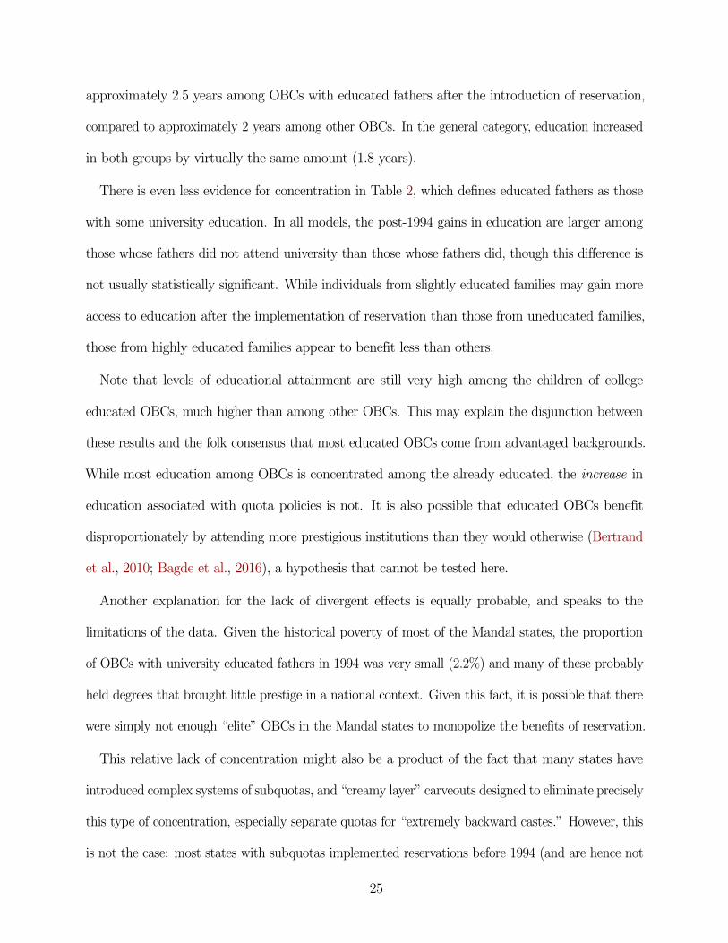
old time threshold (Table C.1). Figures 1a and 1b show these patterns graphically.
Panel B shows the results of a series of linear regression models with government employment as the
dependent variable. The results are substantively similar to those in Panel A. In the DD model, the in-
21

Table 1: Quotas and Socioeconomic Status
(1) (2) (3) (4)VARIABLES 17 17 13 13
Panel A: Years of EducationOBC Caste -2.527*** -2.206***
(0.236) (0.341)Post 1994 -0.375 -0.618**
(0.236) (0.311)OBC*Post 94 0.686* 0.704* 1.140** 1.118***
(0.379) (0.369) (0.446) (0.420)Time Trend 0.132*** 0.153***
(0.0131) (0.0185)OBC*Time Trend 0.00433 -0.00328 -0.0199 -0.0269
(0.0215) (0.0209) (0.0272) (0.0254)
Observations 35,021 35,021 32,477 32,477R-squared 0.094 0.164 0.090 0.159
Panel B: Government JobOBC Caste -0.0792*** -0.0658***
(0.0182) (0.0202)Post 1994 -0.0433** -0.0339
(0.0220) (0.0232)OBC*Post 94 0.0693*** 0.0669** 0.0704*** 0.0554**
(0.0222) (0.0261) (0.0221) (0.0241)Time Trend -0.00472*** -0.00415**
(0.00145) (0.00173)OBC*Time Trend -0.00265** -0.00380** -0.00270* -0.00421**
(0.00132) (0.00173) (0.00140) (0.00174)
Observations 8,784 8,784 7,915 7,915R-squared 0.040 0.170 0.032 0.149State-Caste Category FE NO YES NO YESState-Birth Year FE NO YES NO YESCaste Category-Birth Year FE NO NO NO NO
Robust standard errors in parentheses*** p<0.01, ** p<0.05, * p<0.1
Notes: The tables show the estimates from linear regression models with individual years of education and an indicatorfor government employment as the dependent variables. “Post 94” refers to the year respondents turned 17 or 13, asnoted in the column headings. All models are weighted for sampling probability and have standard errors clustered byhousehold. ∗∗∗p<0.01, ∗∗p<0.05, ∗p<0.1.
troduction of OBC reservations is associated with an increase in the probability of government employ-
ment for OBCs who turn 18 after the adoption of reservations. The increase in the conditional probabil-
ity of a government job in the treatment group is 7 percentage points in the DDmodel, a quite large sub-
stantive effect compared to the full sample average of 13%. The contrast between the small increase in
government employment among OBCs and the gradual decline among non-OBCs is apparent in Figure
22

1c. OBCs were being welcomed into the public sector right when the public sector ceased to have the
central role in the economy it previously had. The results echo the conclusions from a visual inspection
of Figure 1. While there has been a trend towards convergence of OBC and non-OBC outcomes in the
Mandal states, this trend only became more marked for those who came of age some years after 1994.
The effects of government employment in the DDD models (Table C.2) are quite different, being
negative in sign (though not generally statistically significant). The reason for this difference is
evident when we compare Figures 1c and 1d. In the Mandal states, government employment was
declining in parallel before 1994, and converging afterwards. However, in the non-Mandal states,
the pretrends were not parallel; general category government employment was declining much more
rapidly than among OBCs before 1994, and the trend continued afterwards, with OBCs in the
youngest age cohorts actually having higher levels of the state employment than members of the
general category. The relative improvement of OBC position in states that already had quotas
indicate that it is possible that OBC state employment might have improved for political reasons
even without the introduction of quotas, though there is no sign of this in the Mandal state pretrends.
It is also possible that the continuing effects of quotas in the non-Mandal states was larger than the
initial effects of quotas in the Mandal state, leading to the null or negative estimates (see Section 4.4.)
One final interesting aspect of these models is that there is no evidence for the effects of AA being
zero sum, with gains for OBCs counterbalanced by losses for other groups. Non-OBC achievement
continues its linear decline (government employment) or its linear increase (education) indicating
that any losses by Non-OBCs are relative rather than absolute.
5.2 Critique Two: Concentrated Benefits
Are these benefits concentrated in any one segment of the population? Table 2 reruns the models
in Table 1, but interacts the key independent variables with an additional binary variable for whether
on not the respondent’s father attended school (Panel A) or university (Panel B). Results for
23
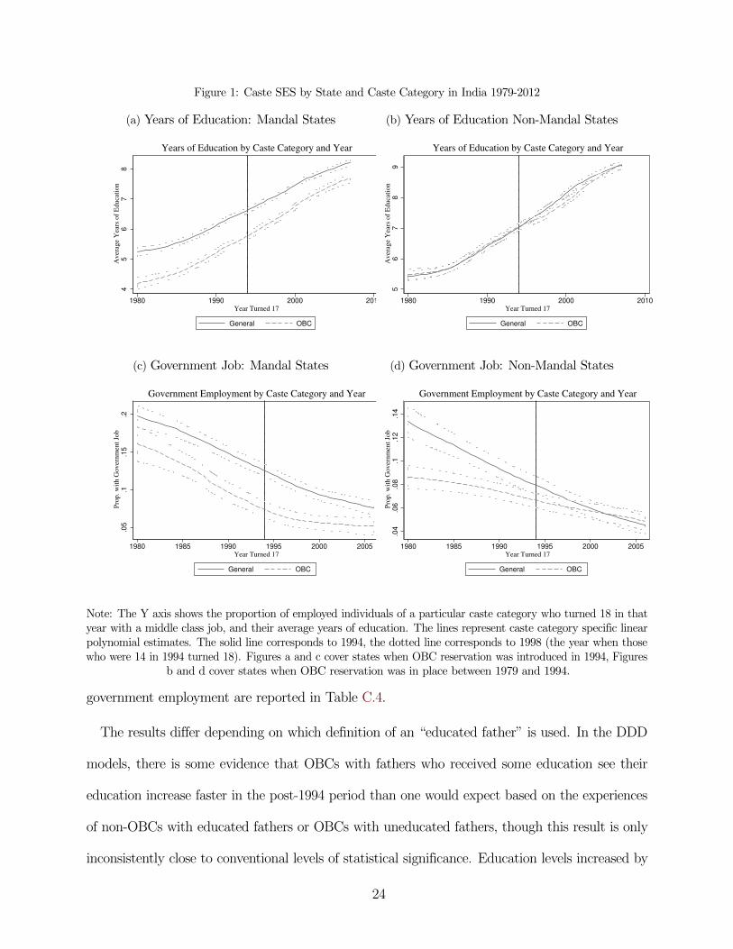
Figure 1: Caste SES by State and Caste Category in India 1979-2012
(a) Years of Education: Mandal States4
56
78
Av
erag
e Y
ears
of
Ed
uca
tio
n
1980 1990 2000 2010
Year Turned 17
General OBC
Years of Education by Caste Category and Year
(b) Years of Education Non-Mandal States
56
78
9
Av
erag
e Y
ears
of
Ed
uca
tio
n
1980 1990 2000 2010
Year Turned 17
General OBC
Years of Education by Caste Category and Year
(c) Government Job: Mandal States
.05
.1.1
5.2
Pro
p.
wit
h G
ov
ern
men
t Jo
b
1980 1985 1990 1995 2000 2005
Year Turned 17
General OBC
Government Employment by Caste Category and Year
(d) Government Job: Non-Mandal States
.04
.06
.08
.1.1
2.1
4
Pro
p.
wit
h G
ov
ern
men
t Jo
b
1980 1985 1990 1995 2000 2005
Year Turned 17
General OBC
Government Employment by Caste Category and Year
Note: The Y axis shows the proportion of employed individuals of a particular caste category who turned 18 in thatyear with a middle class job, and their average years of education. The lines represent caste category specific linearpolynomial estimates. The solid line corresponds to 1994, the dotted line corresponds to 1998 (the year when thosewho were 14 in 1994 turned 18). Figures a and c cover states when OBC reservation was introduced in 1994, Figures
b and d cover states when OBC reservation was in place between 1979 and 1994.
government employment are reported in Table C.4.
The results differ depending on which definition of an “educated father” is used. In the DDD
models, there is some evidence that OBCs with fathers who received some education see their
education increase faster in the post-1994 period than one would expect based on the experiences
of non-OBCs with educated fathers or OBCs with uneducated fathers, though this result is only
inconsistently close to conventional levels of statistical significance. Education levels increased by
24
approximately 2.5 years among OBCs with educated fathers after the introduction of reservation,
compared to approximately 2 years among other OBCs. In the general category, education increased
in both groups by virtually the same amount (1.8 years).
There is even less evidence for concentration in Table 2, which defines educated fathers as those
with some university education. In all models, the post-1994 gains in education are larger among
those whose fathers did not attend university than those whose fathers did, though this difference is
not usually statistically significant. While individuals from slightly educated families may gain more
access to education after the implementation of reservation than those from uneducated families,
those from highly educated families appear to benefit less than others.
Note that levels of educational attainment are still very high among the children of college
educated OBCs, much higher than among other OBCs. This may explain the disjunction between
these results and the folk consensus that most educated OBCs come from advantaged backgrounds.
While most education among OBCs is concentrated among the already educated, the increase in
education associated with quota policies is not. It is also possible that educated OBCs benefit
disproportionately by attending more prestigious institutions than they would otherwise (Bertrand
et al., 2010; Bagde et al., 2016), a hypothesis that cannot be tested here.
Another explanation for the lack of divergent effects is equally probable, and speaks to the
limitations of the data. Given the historical poverty of most of the Mandal states, the proportion
of OBCs with university educated fathers in 1994 was very small (2.2%) and many of these probably
held degrees that brought little prestige in a national context. Given this fact, it is possible that there
were simply not enough “elite” OBCs in the Mandal states to monopolize the benefits of reservation.
This relative lack of concentration might also be a product of the fact that many states have
introduced complex systems of subquotas, and “creamy layer” carveouts designed to eliminate precisely
this type of concentration, especially separate quotas for “extremely backward castes.” However, this
is not the case: most states with subquotas implemented reservations before 1994 (and are hence not
25

Table 2: Quotas, Education and Paternal Education
(1) (2) (3) (4)VARIABLES 17 17 13 13
Panel A: Fathers with Any Education
Post 94 1.027*** 0.930***(0.192) (0.199)
Ed. Father 4.616*** 4.586***(0.197) (0.175)
Post 94*Ed. Father 0.408 0.558**(0.249) (0.252)
OBC -0.892*** -0.887***(0.179) (0.165)
Post 94*OBC 0.459* 0.308 0.676*** 0.637**(0.247) (0.293) (0.261) (0.307)
Ed. Father*OBC -1.392*** -1.357***(0.275) (0.240)
Post 94*Ed. Father*OBC 0.391 0.763* 0.208 0.421(0.344) (0.390) (0.338) (0.385)
Observations 27,044 27,044 27,044 27,044R-squared 0.247 0.326 0.252 0.326Panel B: University Educated FathersPost 94 1.890*** 1.945***
(0.143) (0.144)Ed. Father 6.803*** 6.691***
(0.275) (0.236)Post 94*Ed. Father -1.683*** -1.830***
(0.308) (0.284)OBC -1.980*** -1.987***
(0.150) (0.134)Post 94*OBC 0.648*** 0.587*** 0.829*** 0.860***
(0.185) (0.201) (0.184) (0.192)Ed. Father*OBC 1.072* 1.162**
(0.593) (0.514)Post 94*Ed. Father*OBC -0.883 -0.343 -1.199** -0.939
(0.643) (0.662) (0.591) (0.592)Observations 27,044 27,044 27,044 27,044R-squared 0.141 0.238 0.141 0.239
State-Caste Category*Ed Father FE NO YES NO YESState-Birth Year*Ed Father FE NO YES NO YES
Robust standard errors in parentheses*** p<0.01, ** p<0.05, * p<0.1
Notes: The tables show the estimates from linear regression models with individual years of education as the dependentvariable. “Post 94” refers to the year respondents turned 17 or 13, as noted in the column headings. All models areweighted for sampling probability and have standard errors clustered by household. Educated fathers are those withmore than a secondary education (Panel A), or any education (Panel B). ∗∗∗p<0.01, ∗∗p<0.05, ∗p<0.1.
in the sample), and the exclusion of the few state-years with these policies does not effect the results
(available on request). Section 5.4 shows that the results are similar once the creamy layer is excluded.
26

Do non-beneficiaries at least gain social contact with some of the beneficiaries? Table 3 reports the
marginal effects of a model with a measure of contact with teachers, doctors, police inspectors and
gazetted civil servants among non-university graduates. The results fit with the idea that at least
social networks are being enriched in relative terms, if not absolute ones: The estimated conditional
effect of reservation on social contacts is positive. These results are much stronger, and statistically
significant, using the alternative (age 13) treatment cutoff. Conditional on time trends, the gap
between OBCs and others in contact possession was reduced from 13.2 percentage points among
those who turned 13 before 1994 to 1.3 percentage points among those who turned 13 afterwards.
Table 3: Quotas and Social Contacts
(1) (2) (3) (4)VARIABLES 17 17 13 13
OBC Caste -0.144*** -0.132***(0.0304) (0.0418)
Post 1994 -0.0262 -0.0729**(0.0361) (0.0362)
OBC*Post 94 0.0276 0.0196 0.117** 0.119**(0.0580) (0.0596) (0.0563) (0.0596)
Time Trend -0.000451 0.00132(0.00190) (0.00197)
OBC*Time Trend 0.000619 0.00107 -0.00252 -0.00197(0.00326) (0.00331) (0.00344) (0.00354)
Observations 30,966 30,966 28,695 28,695R-squared 0.014 0.062 0.015 0.061State-Caste Category FE NO YES NO YESState-Birth Year FE NO YES NO YESCaste Category-Birth Year FE NO NO NO NO
Robust standard errors in parentheses*** p<0.01, ** p<0.05, * p<0.1
Notes: The table shows the estimates from linear regression models with an indicator for whetherthe respondent lives in a household where a member knows a doctor, teacher police inspector or gazetted government
officer as the dependent variable. “Post 94” refers to the year respondents turned 17 or 13, as noted in thecolumn headings. All models are weighted for sampling probability and have standard errors clustered by household.
Figure 2a shows that while post-treatment convergence in contacts between caste categories is
a very marked trend, it is centered in the Mandal states and only becomes noticeable around 1994.
While trends were roughly parallel (and, like government employment overall, declining, before 1994
and in the non-Mandal states, after 1994 in the Mandal the level of contacts among OBCs rose even
27

Figure 2: Social Contacts by Caste Category in India 1979-2012
(a) Social Contacts: Mandal States.3
6.3
8.4
.42
.44
.46
Pro
p.
wit
h S
ame
Jati
Go
v.
Co
nta
ct
1980 1990 2000 2010
Year Turned 17
General OBC
Senior Government Contact by Caste Category and Year
(b) Social Contacts: Non-Mandal States
.34
.36
.38
.4.4
2
Pro
p.
wit
h S
ame
Jati
Go
v.
Co
nta
ct
1980 1990 2000 2010
Year Turned 17
General OBC
Senior Government Contact by Caste Category and Year
Note: The Y axis shows the proportion of individuals of a particular caste category who turned 18 in that year wholive in a household where a member knows a doctor, teacher police inspector or gazetted government officer . Thelines represent caste category specific linear polynomial estimates. The solid line corresponds to 1994, the dotted linecorresponds to 1998. Figure b plots the results of the effect of OBC status by year from a set of bivariant regressionmodels within Mandal states, with middle class job and years of education as the dependent variables, and SEsweighted for sampling probability and have standard errors clustered by household. Figure a covers states when OBCreservation was introduced in 1994, Figure b covers states when OBC reservation was in place between 1979 and 1994.
as that of non-OBCs continued to decline, a trend much more marked than the trends in goverment
employment itself shown in Figure 1c.
Note that these results may represent underestimates of the effects of reservations on contacts.
Since individuals can gain contacts at any time (much more easily than they can change jobs or go
back to school) individuals who came of age before 1994 may know individuals who were educated
under AA afterwards.
5.3 Repeated Cross-Sectional Survey Analysis
There are several potential problems with the use of age cohort membership as an index of
exposure of quotas. Individuals might find some way to take advantage of benefits (particularly
in hiring) even though they turned 18 before their introduction. Differential death or migration
rates across groups might bias estimates, as might retrospective reclassification of group membership.
The obvious way to address these concerns would be to use a panel or a repeated cross-section, that
28
directly measures outcomes in the treated and untreated group before and after treatment.
There are several obstacles, however, to implementing this strategy in the Indian context. The most
direct is that before the national implementation of the Mandal report, OBC status was not socially
salient enough to be included on survey questionnaires: The National Sample Survey did not measure
OBCs until the 55th round (1999-2000) and the National Family Health Survey did not include it until
the 2nd round (1998-9). However, for all NFHS rounds (unlike the NSS) data on the raw responses
to the jati question is available after an application process. I was able to obtain this data, manually
standardized the spellings, and then matched the jatis to the state OBC lists.13 Given the highly
variable terminology Indians use to describe their castes, not to mention the many transliteration
and transcription difficulties in a large national survey, this method excludes many OBCs.
The first round of the NFHS only measured individual education among our outcomes.14 Table
4 reports the results of a series of DD and DDD models with years of educations as the dependent
variable. Quota introduction has a positive and statistically significant relationship with with
educational attainment. The magnitude of the estimates (between .43 and .73 years) is substantial
when we consider that these effects are averages over the entire population between 18 and 40.
5.4 Movement between Categories and the Creamy Layer
The main analysis defined the treatment group (OBCs) as those who self-defined as OBCs in 2012,
less those who self-identified as members of jatis that were added to the OBC category after the
respondent turned 17. However, individuals may move between categories, particularly if they have
an incentive to do so (Rao and Ban, 2007), and affirmative action can provide just such an incentive
(Francis et al., 2012). This might be particularly true because caste categories, unlike jatis, are not
primary social identities. Individuals might either be unaware that their jati is classified as an OBC,
or may decide to classify themselves as members of a category that they feel will bring benefits.
13This is the same method used for the DHS data in Appendix Section G.14 Over time trends are show graphically in Figure A.4.
29

Table 4: Quotas and Education: NFHS Data
(1) (2) (3) (4)VARIABLES Edu. Edu. Edu. Edu.
OBC Caste -1.542*** -0.832***(0.0899) (0.0844)
Post 1994 2.426*** 2.751***(0.0432) (0.0463)
Mandal State -0.448***(0.0586)
OBC Caste*Mandal State -0.710***(0.123)
OBC*Post 94 0.727*** 0.835*** 0.0896(0.0960) (0.103) (0.0929)
Post 94*Mandal State -0.325***(0.0633)
OBC*Post 94*Mandal State 0.637*** 0.431***(0.134) (0.144)
Observations 540,343 540,343 893,896 893,896R-squared 0.029 0.073 0.037 0.109State-Caste Category FE NO YES NO YESYear-State FE NO YES NO YESCaste Category-Year FE NO NO NO YES
Robust standard errors in parentheses*** p<0.01, ** p<0.05, * p<0.1
Notes: The tables show the estimates from linear regression models with individual years of education as the dependentvariable. “Post 94” refers to the year of the survey, as noted in the column headings. The sample excluded STs,SCs, and those under 18 or over 40. Observations are weighted based on sampling probability, and standard errorsclustered by household. ∗∗∗p<0.01, ∗∗p<0.05, ∗p<0.1.
To test whether the results are a product of this type of self-reclassification, Appendix Section
G shows the results of a set of models in which caste category is catagorized based on self-reported
jati. Individuals are coded as being members of a caste category if they are members members of
a jati listed in the OBC lists for that state. Due to variation in terminology, using this method,
only 11% of those who turned 17 before 1994 were OBC, and 12 of those who turned 17 afterwards.
The results in these tables broadly echo those in Section Five.
An additional “categorization problem” is the presence of the creamy layer policy, which means that
some OBCs did not benefit from reservation because their families had too high an income. It is unfor-
tunately not possible to cleanly exclude these individuals, since the IHDS does not include questions
on the respondent’s household income at age 17 (the relevant variable), and even if it were available the
30
widespread faking of income certificates would make such a measure an unreliable guide to who actually
took advantage of the policy. As a rough proxy, Appendix Section H reports results that exclude all
OBCs whose fathers had both a professional occupation15 and had completed secondary school. These
tables produce results that are similar in substantive size and significance to those in the main tables.
5.5 Additional Controls
There are any number of potential factors that might influence individual education, social contacts,
and associational membership. Most however, fall into two categories: They are either perfectly
collinear with the state, birth year and caste category fixed effects included in the main models, or
are potentially causally associated with quotas, and thus post treatment. However, Appendix Section
F includes five additional individual control variables that are arguably assigned independently of
quotas: gender, religion FEs, and father’s years of education. Including these controls in the models
has minimal effects relative to the models in Section Five.
Tables I.1 through I.5 examine two additional hypotheses that might explain changes in the relative
social status of OBCs. The mid-1990s were a period when OBC politicians rose to political prominence
in much of northern India, and also a period of increasing migration to urban centers. Either trend
might explain advances among OBCs in this period, at least if we believe that OBC politicians favor
their coethnics over others and that migration might favor the traditionally marginalized. Tables I.1
through I.5 includes controls for OBC chief ministers and the presence of migrants in the household, and
their interaction with OBC. These tables produce results quite similar to the models in the main text.
6 Conclusion
The imposition of hiring and educational quotas in India appears to have neither ignited a social
revolution nor been an abject failure. While the effects of the programs took some time to be
fully realized, they have been associated with modest increases in individual education, government
15“Managerial,” scientists, government officials, doctors, lawyers and accountants.
31

employment, and levels of social contacts with educated professionals among the uneducated. These
effects do not appear to be concentrated among the children of the very highly educated, though
this many be a product of the specific design of Indian affirmative action policies and the relative
poverty of Indian OBCs. These results do not appear a product of pretrends (which, in the the led
treatment models, appear minimal), political changes, or problems in the classification of individuals.
These results paint a more nuanced, and somewhat more positive, portrayal of the effects of OBC
reservation than that common in many accounts of the issue. It shows that affirmative action tends
neither to redistribute opportunities to those who are too poor a “match” to make use of them,
or are so wealthy that they would always take advantage them: There are real effects throughout
the beneficiary group, though perhaps somewhat smaller at the very bottom. These changes have
the secondary effect of increasing the proportion of individuals with bureaucratic and professional
contacts in their own caste, creating both a potential pool of role models and conferring a real
advantage in a political economy as dependent on personal contacts as India.
The results suggest that affirmative action policies in hiring and education may have positive effects
similar to the better-examined ones in the political sphere. More research is necessary on whether these
results can be extended to other regions or regions with differently designed policies—i.e. “soft” quotas,
no exclusion for the wealthy. Similarly, more research is needed on the interaction between the social ef-
fects of policies on targeted groups (discussed here) and their effect on social and institutional efficiency.
Given the importance of these types of policies in many countries, this is research well worth pursuing.
Bibliography
Arcidiacono, P. (2005). Affirmative action in higher education: How do admission and financial
aid rules affect future earnings? Econometrica, 73(5):1477–1524.
Bagde, S., Epple, D., and Taylor, L. (2016). Does affirmative action work? caste, gender, college
32

quality, and academic success in india. American Economic Review, 106(6):1495–1521.
Bertrand, M., Hanna, R., and Mullainathan, S. (2010). Affirmative action in education: Evidence
from engineering college admissions in india. Journal of Public Economics, 94(1):16–29.
Bhavnani, R. R. and Lee, A. (2018). Local embeddedness and bureaucratic performance: evidence
from india. The Journal of Politics, 80(1):71–87.
Bhavnani, R. R. and Lee, A. (2019). Does affirmative action worsen bureaucratic performance?
evidence from the indian administrative service. American Journal of Political Science.
Cassan, G. (2016). Affirmative action, education and gender: Evidence from india.
http://perso.fundp.ac.be/~gcassan/stuff/area_restriction_removal.pdf.
Cederman, L.-E., Wimmer, A., and Min, B. (2010). Why do ethnic groups rebel? new data and
analysis. World Politics, 62(01):87–119.
Chauchard, S. (2014). Can descriptive representation change beliefs about a stigmatized group?
evidence from rural india. American political Science review, 108(2):403–422.
Chew, D. C. (1992). Civil service pay in South Asia. International Labour Organization.
Desai, S. and Vanneman, R. (2015). India human development survey-ii (ihds-ii), 2011-12.
ICPSR36151-v2.
Deshpande, S. and Yadav, Y. (2006). Redesigning affirmative action: Castes and benefits in higher
education. Economic and Political Weekly, pages 2419–2424.
Dunning, T. and Nilekani, J. (2013). Ethnic quotas and political mobilization: caste, parties, and
distribution in indian village councils. American Political Science Review, 107(01):35–56.
33

Ejdemyr, S., Kramon, E., and Robinson, A. L. (2017). Segregation, ethnic favoritism, and the
strategic targeting of distributive goods1. Comparative Political Studies, 51(9):1111–1143.
Francis, A. M., Tannuri-Pianto, M., et al. (2012). Using brazil’s racial continuum to examine the short-
term effects of affirmative action in higher education. Journal of Human Resources, 47(3):754–784.
Galanter, M. (1984). Competing equalities: law and the backward classes in India. University of
California Press Berkeley.
Hinrichs, P. (2012). The effects of affirmative action bans on college enrollment, educational
attainment, and the demographic composition of universities. Review of Economics and Statistics,
94(3):712–722.
Howard, L. and Prakash, N. (2012). Does employment quota explain occupational choice among
disadvantaged groups? a natural experiment from india. International Review of Applied
Economics, 26(4):489–513.
Jaffrelot, C. (2003). India’s silent revolution. Orient Blackswan.
Jensenius, F. R. (2017). Social justice through inclusion: The consequences of electoral quotas in
India. Oxford University Press.
Karekurve-Ramachandra, V. and Lee, A. (Forthcoming). Do gender quotas hurt less privileged
groups? evidence from india. American Journal of Political Science, 64(4):757–72.
Kennedy, R. (2013). For discrimination: Race, affirmative action, and the law. Pantheon.
Khanna, G. (2018). Does affirmative action incentivize schooling? evidence from india.
https://papers.ssrn.com/sol3/papers.cfm?abstract_id=2246549 .
Kramon, E. and Posner, D. N. (2016). Ethnic favoritism in education in kenya. Quarterly Journal
of Political Science, 11:1–58.
34

Krislov, S. (2012). Representative bureaucracy. Quid Pro Books.
Lee, A. (2018). Ethnic diversity and ethnic discrimination: Explaining local public goods provision.
Comparative Political Studies, 51(10):1351–1383.
Lee, A. (2019). From Hierarchy to Ethnicity: The Politics of Caste in Twentieth Century India.
Cambridge Univ Press.
Lee, A. (2020). Replication data for: Does affirmative action work? evaluating india’s quota system.
https://doi.org/10.7910/DVN/YWKZHJ.
Loury, L. D. and Garman, D. (1993). Affirmative action in higher education. The American
Economic Review, 83(2):99–103.
Massey, D. S., Mooney, M., Torres, K. C., and Charles, C. Z. (2006). Black immigrants and black
natives attending selective colleges and universities in the united states. American Journal of
Education, 113(2):243–271.
Mathur, M. L. (2004). Encyclopaedia of Backward Castes: Mandal, media and aftermath, volume 3.
Gyan Publishing House.
Rao, V. and Ban, R. (2007). The political construction of caste in south india.
https://eml.berkeley.edu/~webfac/bardhan/e271_f07/rao.pdf.
Sander, R. H. (2004). A systemic analysis of affirmative action in american law schools. Stanford
law review, pages 367–483.
Shah, G. (2006). Untouchability in rural India. Sage.
Sowell, T. (2005). Affirmative Action around the world: An Empirical Study. Yale University Press.
35

Suryanarayan, P. (2019). When do the poor vote for the right wing and why: Status hierarchy
and vote choice in the indian states. Comparative Political Studies, 52(2):209–245.
36

Online Appendix
A Additional Figures
Figure A.1: Education by State and Caste Category in India 1979-2012
(a) Non-Mandal State
46
81
0
Av
erag
e Y
ears
of
Ed
uca
tio
n
1980 1990 2000 2010
Year Turned 17
OBC General
Education by Caste Category
(b) Mandal State
24
68
10
Av
erag
e Y
ears
of
Ed
uca
tio
n
1980 1990 2000 2010
Year Turned 17
OBC General
Education by Caste Category
Note: The Y axis shows the average years of education for those over 23 for individuals of a particular caste categoryborn in that year. The solid line corresponds to 1994, the dotted line corresponds to 1998 (the year when those who
were 14 in 1994 turned 18).
37

Figure A.2: Middle Class Employment by State and Caste Category in India 1979-2007
(a) Non-Mandal State
0.0
5.1
.15
.2
Go
ver
nm
ent
Em
plo
ym
ent
1980 1990 2000 2010
Year Turned 17
OBC General
Government Employment by Caste Category
(b) Mandal State
0.1
.2.3
Go
ver
nm
ent
Em
plo
ym
ent
1980 1990 2000 2010
Year Turned 17
OBC General
Government Employment by Caste Category
Note: The Y axis shows the proportion of employed individuals of a particular caste category who turned 18 in thatyear who have a middle class job. The solid line corresponds to 1994, the dotted line corresponds to 1998 (the year
when those who were 14 in 1994 turned 18).
Figure A.3: Social Contacts by State and Caste Category in India 1979-2012
(a) Non-Mandal State
.3.3
5.4
.45
Pro
p.
wit
h P
rof.
Co
nta
ct
1980 1990 2000 2010
Year Turned 17
OBC General
Within−Category Contacts by Caste Category
(b) Mandal State
.35
.4.4
5.5
Pro
p.
wit
h P
rof.
Co
nta
ct
1980 1990 2000 2010
Year Turned 17
OBC General
Within−Category Contacts by Caste Category
Note: The Y axis shows the proportion of individuals of a particular caste category who turned 18 in that year wholive in a household where a member knows a doctor, teacher police inspector or gazetted government officer. The solidline corresponds to 1994, the dotted line corresponds to 1998 (the year when those who were 14 in 1994 turned 18).
38
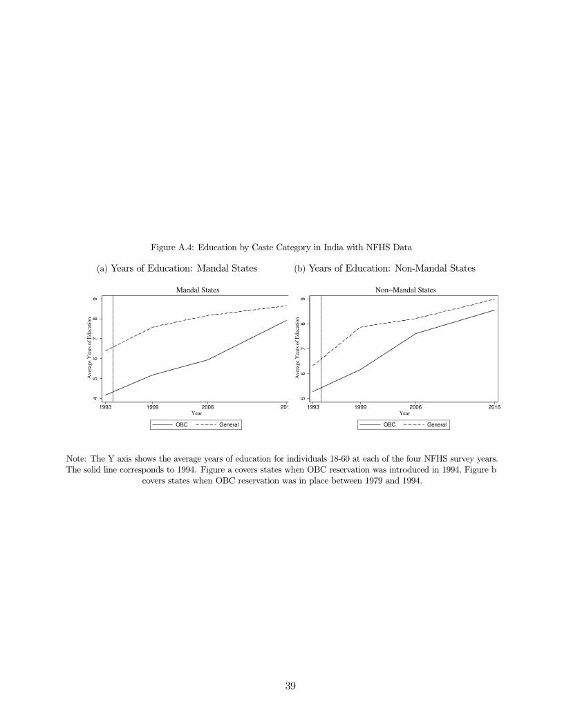
Figure A.4: Education by Caste Category in India with NFHS Data
(a) Years of Education: Mandal States
45
67
89
Av
erag
e Y
ears
of
Ed
uca
tio
n
1993 1999 2006 2016
Year
OBC General
Mandal States
(b) Years of Education: Non-Mandal States
56
78
9
Av
erag
e Y
ears
of
Ed
uca
tio
n
1993 1999 2006 2016
Year
OBC General
Non−Mandal States
Note: The Y axis shows the average years of education for individuals 18-60 at each of the four NFHS survey years.The solid line corresponds to 1994. Figure a covers states when OBC reservation was introduced in 1994, Figure b
covers states when OBC reservation was in place between 1979 and 1994.
39
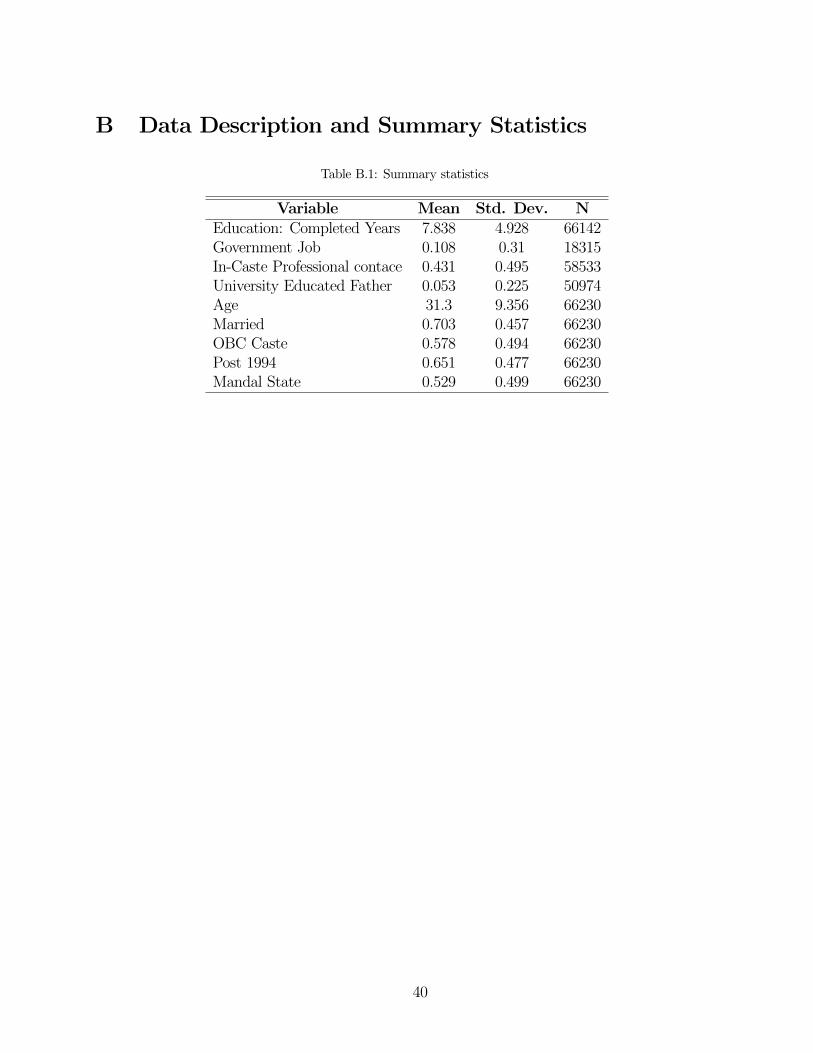
B Data Description and Summary Statistics
Table B.1: Summary statistics
Variable Mean Std. Dev. NEducation: Completed Years 7.838 4.928 66142Government Job 0.108 0.31 18315In-Caste Professional contace 0.431 0.495 58533University Educated Father 0.053 0.225 50974Age 31.3 9.356 66230Married 0.703 0.457 66230OBC Caste 0.578 0.494 66230Post 1994 0.651 0.477 66230Mandal State 0.529 0.499 66230
40

Table B.2: OBC Reservations in India: A Summary
State SomeColonialRes.
Post1947 Res.Began
2011 OBCQuota
SubquotaYear
Notes
AndhraPradesh
Yes 1947 23% 1970 System reformed on state reorga-nization 1964
Tamil Nadu Yes 1947 68% 1989 Quota expanded from 25% before1971 and 31% before 1980
Maharashtra Yes 1947 32% 1964 System reformed on state reorga-nization 1964
Kerala Yes 1964 40%Punjab No 1964 12% Quota 5% before 1993Karnataka Yes 1977 32% 1977 50% quota pre-1956, changed to
class-based 1961, 35% 1977, 55’%quota 1986, 32% quota 1994
Bihar No 1978 33% 1978 Quota increased from 20% in 1992Gujarat Yes 1978 27% Some quotas pre-1964, before states
reorganizationJharkhand No 1978 14% 1978 Quota shrunk from 33% in 2000 on
state reorganizationHaryana No 1991 27% 1995 Class-based res. from 1969Assam No 1994 27%Chhattisgarh No 1994 14%Delhi No 1994 27%Goa No 1994 19.5%HimachalPradesh
No 1994 20% Class-based res. from 1970
MadhyaPradesh
No 1994 14%
Manipur No 1994 17%Orissa No 1994 12%Rajasthan No 1994 21%Sikkim No 1994 23%Uttar Pradesh No 1994 27%Uttarakhand No 1994 14% Quota shrunk from 27% in 2000 on
state reorganizationWest Bengal No 1994 7%
Tripura, Meghalaya, Mizoram and Arunachal Pradesh do not have OBC reservations, Jammu and Kashmir hasclass-based reservations. Union territories are not included for reasons of space. Sources: See .
41

C DDD Models
Table C.1: Quotas and Education
(1) (2) (3) (4)VARIABLES 17 17 13 13
OBC Caste -1.993*** -1.854***(0.157) (0.137)
Post 1994 2.188*** 2.375***(0.137) (0.125)
Mandal State -0.653*** -0.555***(0.165) (0.143)
OBC*Post 94 0.486*** 0.325**(0.177) (0.164)
OBC Caste*Mandal State -0.496** -0.591***(0.212) (0.186)
Post 94*Mandal State -0.381** -0.642***(0.182) (0.171)
OBC*Post 94*Mandal State 0.332 0.219 0.586*** 0.527**(0.241) (0.240) (0.226) (0.221)
Observations 66,142 66,142 66,142 66,142R-squared 0.085 0.208 0.092 0.208State-Caste Category FE NO YES NO YESState-Birth Year FE NO YES NO YESCaste Category-Birth Year FE NO YES NO YES
Robust standard errors in parentheses*** p<0.01, ** p<0.05, * p<0.1
Notes: The table shows the results of a series of linear regression models with individual years of education as thedependent variable. “Post 94” refers to the year respondents turned 17 or turned 13, depending on the column heading.All models are weighted for sampling probability and have standard errors clustered by household. ∗∗∗p< 0.01,∗∗p<0.05, ∗p<0.1.
42

Table C.2: Quotas and Government Employment
(1) (2) (3) (4)VARIABLES 17 17 13 13
OBC Caste -0.0856*** -0.0831***(0.0139) (0.0118)
Post 1994 -0.0798*** -0.0929***(0.0158) (0.0141)
Mandal State 0.0517*** 0.0399***(0.0172) (0.0149)
OBC*Post 94 0.0488*** 0.0640***(0.0176) (0.0162)
OBC Caste*Mandal State -0.0141 -0.0139(0.0204) (0.0175)
Post 94*Mandal State -0.0279 -0.00664(0.0214) (0.0202)
OBC*Post 94*Mandal State -0.00842 -0.0343 -0.0191 -0.0500**(0.0250) (0.0260) (0.0238) (0.0247)
Observations 18,315 18,315 18,315 18,315R-squared 0.030 0.130 0.028 0.130State-Caste Category FE NO YES NO YESState-Birth Year FE NO YES NO YESCaste Category-Birth Year FE NO YES NO YES
Robust standard errors in parentheses*** p<0.01, ** p<0.05, * p<0.1
Notes: The table shows the results of a series of linear regression models with an indicator for government employmentas the dependent variable. “Post 94” refers to the year respondents turned 17 or turned 13, depending on the columnheading. All models are weighted for sampling probability and have standard errors clustered by household. Models1-4 correspond to Equations 1-4. ∗∗∗p<0.01, ∗∗p<0.05, ∗p<0.1.
43

Table C.3: Quotas and Within-Caste Professional Contacts
(1) (2) (3) (4)VARIABLES 17 17 13 13
OBC Caste -0.132*** -0.144***(0.0166) (0.0151)
Post 1994 0.0160 0.00539(0.0135) (0.0135)
Mandal State 0.0217 0.0193(0.0178) (0.0167)
OBC*Post 94 -0.0327* -0.0167(0.0171) (0.0168)
OBC Caste*Mandal State -0.00734 -0.00966(0.0236) (0.0215)
Post 94*Mandal State -0.0497*** -0.0561***(0.0186) (0.0190)
OBC*Post 94*Mandal State 0.0706*** 0.0289 0.0892*** 0.0563**(0.0243) (0.0259) (0.0242) (0.0263)
Observations 58,533 58,533 58,533 58,533R-squared 0.018 0.081 0.019 0.081State-Caste Category FE NO YES NO YESState-Birth Year FE NO YES NO YESCaste Category-Birth Year FE NO YES NO YES
Robust standard errors in parentheses*** p<0.01, ** p<0.05, * p<0.1
Notes: The table shows the results of a series of linear regression models with a binary measure for whether someonein the household knows a doctor, teacher police inspector or gazetted government officer as the dependent variable.“Post 94” refers to the year respondents turned 17 or turned 13, depending on the column heading. All modelsare weighted for sampling probability and have standard errors clustered by household. Models 1-4 correspond toEquations 1-4. ∗∗∗p<0.01, ∗∗p<0.05, ∗p<0.1.
44

Table C.4: Quotas, Government Jobs and Paternal Education
(1) (2) (3) (4)VARIABLES 17 17 13 13
Panel A: University Educated FathersPost 94 -0.110*** -0.0924***
(0.0160) (0.0168)Ed. Father 0.278*** 0.292***
(0.0578) (0.0502)Post 94*Ed. Father -0.0757 -0.141**
(0.0718) (0.0691)OBC -0.0895*** -0.0815***
(0.0148) (0.0126)Post 94*OBC 0.0520*** 0.0339 0.0447** 0.0187
(0.0191) (0.0214) (0.132) (0.0206)Ed. Father*OBC 0.0587 -0.0219
(0.122) (0.0970)Post 94*Ed. Father*OBC -0.0479 0.187 0.105 0.142
(0.145) (0.126) (0.145) (0.135)
Observations 7,043 7,043 7,043 7,043R-squared 0.059 0.267 0.059 0.267
Panel B: Fathers with Any Education(1) (2) (3) (4)
VARIABLES 17 17 13 13
Post 94 -0.0521*** -0.0568***(0.0153) (0.0144)
Ed. Father 0.218*** 0.187***(0.0223) (0.0203)
Post 94*Ed. Father -0.126*** -0.0932***(0.0287) (0.0293)
OBC -0.0424*** -0.0360***(0.0135) (0.0125)
Post 94*OBC 0.0342* 0.0259 0.0272 0.0289(0.0190) (0.0220) (0.0181) (0.0210)
Ed. Father*OBC -0.0488 -0.0711***(0.0315) (0.0264)
Post 94*Ed. Father*OBC -0.0107 -0.00782 0.0263 -0.0174(0.0383) (0.0426) (0.0363) (0.0388)
Observations 7,043 7,043 7,043 7,043R-squared 0.084 0.285 0.070 0.285
Observations 27,044 27,044 27,044 27,044R-squared 0.247 0.326 0.252 0.326State-Caste Category*Ed Father FE NO YES NO YESState-Birth Year*Ed Father FE NO YES NO YES
Robust standard errors in parentheses*** p<0.01, ** p<0.05, * p<0.1
Notes: The tables show the estimates from linear regression models with government employment as the dependentvariable. “Post 94” refers to the year respondents turned 17 or 13, as noted in the column headings. All models areweighted for sampling probability and have standard errors clustered by household. Educated fathers are those withmore than a secondary education (Panel A), or any education (Panel B). ∗∗∗p<0.01, ∗∗p<0.05, ∗p<0.1.
45

D Lags
Table D.1: Education: Eight Year Lagged Treatment
(1) (2) (3) (4)VARIABLES yearsofeducation yearsofeducation yearsofeducation yearsofeducation
OBC Caste -2.309*** -1.764***(0.147) (0.146)
Post 1994 1.388*** 1.991***(0.143) (0.136)
Mandal State -0.668***(0.165)
OBC*Post 94 0.943*** 0.844*** 0.398**(0.183) (0.196) (0.176)
OBC Caste*Mandal State -0.545***(0.207)
Post 94*Mandal State -0.603***(0.197)
OBC*Post 94*Mandal State 0.545** 0.607**(0.254) (0.258)
Observations 28,628 28,628 53,474 53,474R-squared 0.070 0.145 0.082 0.190State-Caste Category FE NO YES NO YESState-Birth Year FE NO YES NO YESCaste Category-Birth Year FE NO NO NO YES
Robust standard errors in parentheses*** p<0.01, ** p<0.05, * p<0.1
Notes: The table shows the results of a series of linear regression models with individual years of education as thedependent variable. “Post 94” refers to the year respondents turned 10. Only individuals with fathers who graduatedfrom secondary school are included.All models are weighted for sampling probability and have standard errors clusteredby household. Models 1-4 correspond to Equations 1-4. ∗∗∗p<0.01, ∗∗p<0.05, ∗p<0.1.
46

Table D.2: Government Employment: Eight Year Lagged Treatment
(1) (2) (3) (4)VARIABLES govjob govjob govjob govjob
OBC Caste -0.0850*** -0.0526***(0.0133) (0.0112)
Post 1994 -0.0670*** -0.0483***(0.0172) (0.0152)
Mandal State 0.0396**(0.0154)
OBC*Post 94 0.0441** 0.0409** 0.0310*(0.0202) (0.0207) (0.0181)
OBC Caste*Mandal State -0.0324*(0.0174)
Post 94*Mandal State -0.0187(0.0230)
OBC*Post 94*Mandal State 0.0131 0.0225(0.0271) (0.0263)
Observations 6,624 6,624 13,708 13,708R-squared 0.021 0.128 0.017 0.100State-Caste Category FE NO YES NO YESState-Birth Year FE NO YES NO YESCaste Category-Birth Year FE NO NO NO YES
Robust standard errors in parentheses*** p<0.01, ** p<0.05, * p<0.1
Notes: The table shows the results of a series of linear regression models with an indicator for government employmentas the dependent variable. “Post 94” refers to the year respondents turned 10. All models are weighted for samplingprobability and have standard errors clustered by household. Models 1-4 correspond to Equations 1-4. ∗∗∗p<0.01,∗∗p<0.05, ∗p<0.1.
47

Table D.3: Contacts: Eight Year Lagged Treatment
(1) (2) (3) (4)VARIABLES Caste Contact Caste Contact Caste Contact Caste Contact
OBC Caste -0.143*** -0.153***(0.0171) (0.0171)
Post 1994 -0.0387** 0.00558(0.0173) (0.0168)
Mandal State 0.00468(0.0197)
OBC*Post 94 0.0641*** 0.0693*** -0.00832(0.0213) (0.0249) (0.0208)
OBC Caste*Mandal State 0.0102(0.0242)
Post 94*Mandal State -0.0443*(0.0242)
OBC*Post 94*Mandal State 0.0724** 0.0647**(0.0298) (0.0327)
Observations 25,214 25,214 47,034 47,034R-squared 0.013 0.057 0.018 0.080State-Caste Category FE NO YES NO YESState-Birth Year FE NO YES NO YESCaste Category-Birth Year FE NO NO NO YES
Robust standard errors in parentheses*** p<0.01, ** p<0.05, * p<0.1
Notes: The table shows the results of a series of linear regression models with a binary measure for whether someonein the household knows a doctor, teacher police inspector or gazetted government officer as the dependent variable.“Post 94” refers to the year respondents turned 10. All models are weighted for sampling probability and have standarderrors clustered by household. Models 1-4 correspond to Equations 1-4. ∗∗∗p<0.01, ∗∗p<0.05, ∗p<0.1.
48

D Leads
Table E.1: Education: Four Year Treatment Lead
(1) (2) (3) (4)VARIABLES yearsofeducation yearsofeducation yearsofeducation yearsofeducation
OBC Caste -2.664*** -2.205***(0.144) (0.150)
Post 1994 0.647*** 0.853***(0.184) (0.213)
Mandal State -0.574***(0.157)
OBC*Post 94 0.241 0.328 0.453*(0.247) (0.262) (0.269)
OBC Caste*Mandal State -0.459**(0.208)
Post 94*Mandal State -0.206(0.281)
OBC*Post 94*Mandal State -0.212 -0.0975(0.365) (0.374)
Observations 15,115 15,115 29,631 29,631R-squared 0.066 0.144 0.061 0.164State-Caste Category FE NO YES NO YESState-Birth Year FE NO YES NO YESCaste Category-Birth Year FE NO NO NO YES
Robust standard errors in parentheses*** p<0.01, ** p<0.05, * p<0.1
Notes: The table shows the results of a series of linear regression models with individual years of education as thedependent variable. “Post 94” refers to the year respondents turned 21. Only individuals with fathers who graduatedfrom secondary school are included.All models are weighted for sampling probability and have standard errors clusteredby household. Models 1-4 correspond to Equations 1-4. ∗∗∗p<0.01, ∗∗p<0.05, ∗p<0.1.
49
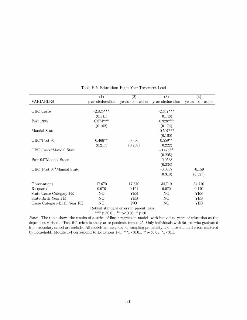
Table E.2: Education: Eight Year Treatment Lead
(1) (2) (3) (4)VARIABLES yearsofeducation yearsofeducation yearsofeducation yearsofeducation
OBC Caste -2.825*** -2.347***(0.141) (0.148)
Post 1994 0.874*** 0.928***(0.162) (0.174)
Mandal State -0.597***(0.160)
OBC*Post 94 0.466** 0.336 0.559**(0.217) (0.238) (0.222)
OBC Caste*Mandal State -0.478**(0.205)
Post 94*Mandal State -0.0538(0.238)
OBC*Post 94*Mandal State -0.0937 -0.159(0.310) (0.327)
Observations 17,670 17,670 34,710 34,710R-squared 0.076 0.154 0.070 0.170State-Caste Category FE NO YES NO YESState-Birth Year FE NO YES NO YESCaste Category-Birth Year FE NO NO NO YES
Robust standard errors in parentheses*** p<0.01, ** p<0.05, * p<0.1
Notes: The table shows the results of a series of linear regression models with individual years of education as thedependent variable. “Post 94” refers to the year respondents turned 25. Only individuals with fathers who graduatedfrom secondary school are included.All models are weighted for sampling probability and have standard errors clusteredby household. Models 1-4 correspond to Equations 1-4. ∗∗∗p<0.01, ∗∗p<0.05, ∗p<0.1.
50

Table E.3: Government Employment: Four Year Treatment Lead
(1) (2) (3) (4)VARIABLES govjob govjob govjob govjob
OBC Caste -0.104*** -0.0899***(0.0182) (0.0157)
Post 1994 -0.0897*** -0.0633***(0.0229) (0.0219)
Mandal State 0.0747***(0.0191)
OBC*Post 94 0.00477 0.0437 0.0204(0.0277) (0.0311) (0.0242)
OBC Caste*Mandal State -0.0143(0.0240)
Post 94*Mandal State -0.0265(0.0316)
OBC*Post 94*Mandal State -0.0156 0.0211(0.0368) (0.0383)
Observations 5,109 5,109 10,836 10,836R-squared 0.029 0.202 0.034 0.158State-Caste Category FE NO YES NO YESState-Birth Year FE NO YES NO YESCaste Category-Birth Year FE NO NO NO YES
Robust standard errors in parentheses*** p<0.01, ** p<0.05, * p<0.1
Notes: The table shows the results of a series of linear regression models with an indicator for government employmentas the dependent variable. “Post 94” refers to the year respondents turned 21. All models are weighted for samplingprobability and have standard errors clustered by household. Models 1-4 correspond to Equations 1-4. ∗∗∗p<0.01,∗∗p<0.05, ∗p<0.1.
51

Table E.4: Government Employment: Eight Year Treatment Lead
(1) (2) (3) (4)VARIABLES govjob govjob govjob govjob
OBC Caste -0.143*** -0.109***(0.0202) (0.0175)
Post 1994 -0.132*** -0.0997***(0.0208) (0.0208)
Mandal State 0.0907***(0.0218)
OBC*Post 94 0.0521* 0.0699** 0.0478**(0.0267) (0.0296) (0.0232)
OBC Caste*Mandal State -0.0338(0.0268)
Post 94*Mandal State -0.0323(0.0294)
OBC*Post 94*Mandal State 0.00431 0.0340(0.0353) (0.0371)
Observations 5,790 5,790 12,295 12,295R-squared 0.040 0.214 0.043 0.167State-Caste Category FE NO YES NO YESState-Birth Year FE NO YES NO YESCaste Category-Birth Year FE NO NO NO YES
Robust standard errors in parentheses*** p<0.01, ** p<0.05, * p<0.1
Notes: The table shows the results of a series of linear regression models with an indicator for government employmentas the dependent variable. “Post 94” refers to the year respondents turned 25. All models are weighted for samplingprobability and have standard errors clustered by household. Models 1-4 correspond to Equations 1-4. ∗∗∗p<0.01,∗∗p<0.05, ∗p<0.1.
52

Table E.5: Contacts: Four Year Treatment Lead
(1) (2) (3) (4)VARIABLES Caste Contact Caste Contact Caste Contact Caste Contact
OBC Caste -0.130*** -0.139***(0.0186) (0.0168)
Post 1994 -0.0152 -0.0284(0.0200) (0.0213)
Mandal State 0.00785(0.0188)
OBC*Post 94 -0.0196 -0.0288 0.0101(0.0272) (0.0299) (0.0263)
OBC Caste*Mandal State 0.00879(0.0250)
Post 94*Mandal State 0.0132(0.0293)
OBC*Post 94*Mandal State -0.0297 -0.0544(0.0378) (0.0398)
Observations 13,522 13,522 26,765 26,765R-squared 0.019 0.081 0.019 0.090State-Caste Category FE NO YES NO YESState-Birth Year FE NO YES NO YESCaste Category-Birth Year FE NO NO NO YES
Robust standard errors in parentheses*** p<0.01, ** p<0.05, * p<0.1
Notes: The table shows the results of a series of linear regression models with a binary measure for whether someonein the household knows a doctor, teacher police inspector or gazetted government officer as the dependent variable.“Post 94” refers to the year respondents turned 21. All models are weighted for sampling probability and have standarderrors clustered by household. Models 1-4 correspond to Equations 1-4. ∗∗∗p<0.01, ∗∗p<0.05, ∗p<0.1.
53

Table E.6: Contacts: Eight Year Treatment Lead
(1) (2) (3) (4)VARIABLES Caste Contact Caste Contact Caste Contact Caste Contact
OBC Caste -0.124*** -0.155***(0.0195) (0.0167)
Post 1994 -0.00314 -0.0317*(0.0186) (0.0181)
Mandal State -0.00478(0.0198)
OBC*Post 94 -0.0207 -0.0356 0.0273(0.0252) (0.0279) (0.0227)
OBC Caste*Mandal State 0.0307(0.0257)
Post 94*Mandal State 0.0285(0.0260)
OBC*Post 94*Mandal State -0.0479 -0.0664*(0.0339) (0.0358)
Observations 15,895 15,895 31,503 31,503R-squared 0.018 0.082 0.020 0.091State-Caste Category FE NO YES NO YESState-Birth Year FE NO YES NO YESCaste Category-Birth Year FE NO NO NO YES
Robust standard errors in parentheses*** p<0.01, ** p<0.05, * p<0.1
Notes: The table shows the results of a series of linear regression models with a binary measure for whether someonein the household knows a doctor, teacher police inspector or gazetted government officer as the dependent variable.“Post 94” refers to the year respondents turned 25. All models are weighted for sampling probability and have standarderrors clustered by household. Models 1-4 correspond to Equations 1-4. ∗∗∗p<0.01, ∗∗p<0.05, ∗p<0.1.
54

F Controls
Table F.1: Education: Controls
(1) (2) (3) (4)VARIABLES Age 17 Treat. Age 17 Treat. Age 13 Treat. Age 13 Treat.OBC Caste -1.388*** -1.329***
(0.128) (0.125)Post 1994 1.070*** 1.134***
(0.105) (0.109)OBC*Post 94 0.558*** 0.603*** 0.582*** 0.653***
(0.150) (0.168) (0.153) (0.169)
Observations 27,044 27,044 24,778 24,778R-squared 0.384 0.428 0.381 0.423Controls YES YES YES YESState-Caste Category FE NO YES NO YESState-Birth Year FE NO YES NO YESCaste Category-Birth Year FE NO YES NO YES
Robust standard errors in parentheses*** p<0.01, ** p<0.05, * p<0.1
Notes: The table shows the results of a series of linear regression models with individual years of education as thedependent variable. “Post 94” refers to the year respondents turned 17 or turned 13, depending on the columnheading. All models include controls for gender, urban residence, size of household, number on men and women in thehousehold, and religion dummies. Only individuals with fathers who graduated from secondary school are included.Allmodels are weighted for sampling probability and have standard errors clustered by household. Models 1-4 correspondto Equations 1-4.
55
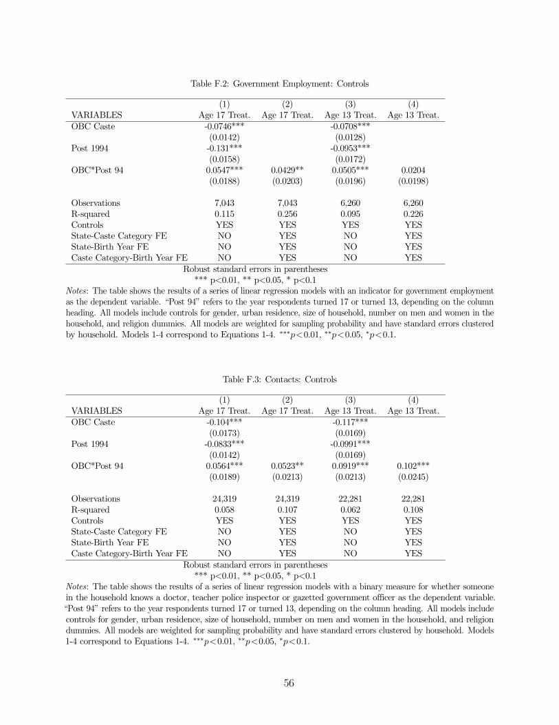
Table F.2: Government Employment: Controls
(1) (2) (3) (4)VARIABLES Age 17 Treat. Age 17 Treat. Age 13 Treat. Age 13 Treat.OBC Caste -0.0746*** -0.0708***
(0.0142) (0.0128)Post 1994 -0.131*** -0.0953***
(0.0158) (0.0172)OBC*Post 94 0.0547*** 0.0429** 0.0505*** 0.0204
(0.0188) (0.0203) (0.0196) (0.0198)
Observations 7,043 7,043 6,260 6,260R-squared 0.115 0.256 0.095 0.226Controls YES YES YES YESState-Caste Category FE NO YES NO YESState-Birth Year FE NO YES NO YESCaste Category-Birth Year FE NO YES NO YES
Robust standard errors in parentheses*** p<0.01, ** p<0.05, * p<0.1
Notes: The table shows the results of a series of linear regression models with an indicator for government employmentas the dependent variable. “Post 94” refers to the year respondents turned 17 or turned 13, depending on the columnheading. All models include controls for gender, urban residence, size of household, number on men and women in thehousehold, and religion dummies. All models are weighted for sampling probability and have standard errors clusteredby household. Models 1-4 correspond to Equations 1-4. ∗∗∗p<0.01, ∗∗p<0.05, ∗p<0.1.
Table F.3: Contacts: Controls
(1) (2) (3) (4)VARIABLES Age 17 Treat. Age 17 Treat. Age 13 Treat. Age 13 Treat.OBC Caste -0.104*** -0.117***
(0.0173) (0.0169)Post 1994 -0.0833*** -0.0991***
(0.0142) (0.0169)OBC*Post 94 0.0564*** 0.0523** 0.0919*** 0.102***
(0.0189) (0.0213) (0.0213) (0.0245)
Observations 24,319 24,319 22,281 22,281R-squared 0.058 0.107 0.062 0.108Controls YES YES YES YESState-Caste Category FE NO YES NO YESState-Birth Year FE NO YES NO YESCaste Category-Birth Year FE NO YES NO YES
Robust standard errors in parentheses*** p<0.01, ** p<0.05, * p<0.1
Notes: The table shows the results of a series of linear regression models with a binary measure for whether someonein the household knows a doctor, teacher police inspector or gazetted government officer as the dependent variable.“Post 94” refers to the year respondents turned 17 or turned 13, depending on the column heading. All models includecontrols for gender, urban residence, size of household, number on men and women in the household, and religiondummies. All models are weighted for sampling probability and have standard errors clustered by household. Models1-4 correspond to Equations 1-4. ∗∗∗p<0.01, ∗∗p<0.05, ∗p<0.1.
56

Table F.4: Differential Effects on Education: Controls
(1) (2) (3) (4)VARIABLES 17 17 13 13
Panel A: Fathers with University EducationPost 1994 1.116*** 1.205***
(0.111) (0.110)Ed. Father 0.441 0.507**
(0.279) (0.247)Post 94*Ed. Father -0.787*** -0.907***
(0.285) (0.259)OBC Caste -1.368*** -1.355***
(0.131) (0.116)Post 94*OBC Caste 0.534*** 0.609***
(0.156) (0.152)Ed. Father*OBC Caste 0.441 0.542
(0.551) (0.488)Post 94*Ed. Father*OBC -0.709 -0.959*
(0.599) (0.564)
Observations 27,044 27,044 27,044 27,044R-squared 0.384 0.435 0.389 0.436Panel B: Fathers with Any EducationPost 1994 = 1 1.346*** 1.271***
(0.183) (0.196)Ed. Father 0.530** 0.382**
(0.212) (0.195)1.temp int post94#Ed. Father -0.465** -0.231
(0.232) (0.239)OBC Caste = 1 -1.201*** -1.198***
(0.182) (0.167)1.temp int post94#1.temp int*OBC 0.350 0.732*** 0.537** 0.593**
(0.238) (0.207) (0.257) (0.282)Ed. Father*1.temp int*OBC -0.321 -0.328
(0.259) (0.226)1.temp int post94#Ed. Father*1.temp int*OBC 0.327 -0.258 0.198 0.306
(0.323) (0.233) (0.322) (0.352)
Observations 27,044 27,044 27,044 27,044R-squared 0.384 0.438 0.388 0.445State-Caste Category*Ed Father FE NO YES NO YESState-Birth Year*Ed Father FE NO YES NO YES
Robust standard errors in parentheses*** p<0.01, ** p<0.05, * p<0.1
Notes: The table shows the results of a series of linear regression models with individual years of education as thedependent variable. OBCs are defined as those belonging to a state-jati where over 90% of jati members identifyas OBC. “Post 94” refers to the year respondents turned 17 or 13, as noted in the column headings. All modelsinclude controls for gender, urban residence, size of household, number on men and women in the household, andreligion dummies. All models are weighted for sampling probability and have standard errors clustered by household.∗∗∗p<0.01, ∗∗p<0.05, ∗p<0.1.
57

Table F.5: Differential Effects on Government Employment: Controls
(1) (2) (3) (4)VARIABLES 17 17 13 13
Panel A: Fathers with University EducationPost 1994 -0.108*** -0.108***
(0.0175) (0.0175)Ed.Father 0.0766 0.0766
(0.0540) (0.0540)Post 94*Ed.Father -0.134** -0.134**
(0.0684) (0.0684)OBC Caste -0.0668*** -0.0668***
(0.0125) (0.0125)Post 94*OBC Caste 0.0430** 0.0430**
(0.0198) (0.0198)Ed.Father *OBC Caste -0.0429 -0.0429
(0.0964) (0.0964)Post 94*Ed.Father*OBC 0.124 0.124
(0.131) (0.131)
Observations 7,043 7,043 7,043 7,043R-squared 0.109 0.308 0.109 0.308Panel B: Fathers with Any Education
Post 1994 = 1 -0.0512*** -0.0573***(0.0150) (0.0147)
Ed. Father 0.0327 0.00366(0.0268) (0.0248)
1.temp int post94#Ed. Father -0.145*** -0.107***(0.0281) (0.0296)
OBC Caste = 1 -0.0569*** -0.0519***(0.0143) (0.0129)
1.temp int post94#1.temp int*OBC 0.0365* 0.0880*** 0.0335* 0.0361*(0.0188) (0.0208) (0.0182) (0.0216)
Ed. Father*1.temp int*OBC -0.00445 -0.0255(0.0307) (0.0260)
1.temp int post94#Ed. Father*1.temp int*OBC -0.0105 -0.118*** 0.0181 -0.0264(0.0372) (0.0245) (0.0359) (0.0387)
Observations 7,043 7,043 7,043 7,043R-squared 0.131 0.316 0.115 0.316
Observations 27,044 27,044 27,044 27,044R-squared 0.384 0.438 0.388 0.445
Observations 7,043 7,043 7,043 7,043R-squared 0.131 0.316 0.115 0.316State-Caste Category*Ed Father FE NO YES NO YESState-Birth Year*Ed Father FE NO YES NO YES
Robust standard errors in parentheses*** p<0.01, ** p<0.05, * p<0.1
Notes: The table shows the results of a series of linear regression models with government employment as thedependent variable. OBCs are defined as those belonging to a state-jati where over 90% of jati members identifyas OBC. “Post 94” refers to the year respondents turned 17 or 13, as noted in the column headings. All modelsinclude controls for gender, urban residence, size of household, number on men and women in the household, andreligion dummies. All models are weighted for sampling probability and have standard errors clustered by household.∗∗∗p<0.01, ∗∗p<0.05, ∗p<0.1.
58

G Individual Movement between Categories
Table G.1: Education: Caste Category Defined by Jati
(1) (2) (3) (4)VARIABLES 17 17 13 13
OBC Caste -1.466*** -1.178***(0.155) (0.151)
Post 1994 -0.408*** -0.376**(0.156) (0.169)
OBC*Post 94 1.667*** 1.374*** 1.569*** 1.327***(0.185) (0.187) (0.183) (0.183)
Time Trend 0.174*** -0.309 0.183*** -0.317(0.00755) (0.863) (0.00929) (0.857)
OBC*Time Trend -0.0744*** -0.0814*** -0.0738*** -0.0806***(0.00488) (0.00535) (0.00488) (0.00534)
Observations 35,021 35,021 32,477 32,477R-squared 0.083 0.146 0.082 0.144State-Caste Category FE NO YES NO YESState-Birth Year FE NO YES NO YESCaste Category-Birth Year FE NO NO NO NO
Robust standard errors in parentheses*** p<0.01, ** p<0.05, * p<0.1
Notes: The table shows the results of a series of linear regression models with individual years of education as thedependent variable. OBCs are defined as those belonging to a state-jati where over 90% of jati members identify asOBC. “Post 94” refers to the year respondents turned 17 or 13. All models are weighted for sampling probability andhave standard errors clustered by household. ∗∗∗p<0.01, ∗∗p<0.05, ∗p<0.1.
59

Table G.2: Government Employment: Caste Category Defined by Jati
(1) (2) (3) (4)VARIABLES 17 17 13 13
OBC Caste -0.0388** -0.0125(0.0175) (0.0166)
Post 1994 -0.0254 -0.00818(0.0172) (0.0183)
OBC*Post 94 0.0851*** 0.0675*** 0.0664*** 0.0363(0.0212) (0.0208) (0.0241) (0.0232)
Time Trend -0.00371*** 0.00453*** -0.00335** 0.00438***(0.00122) (0.000740) (0.00145) (0.000743)
OBC*Time Trend -0.00440*** -0.00453*** -0.00435*** -0.00438***(0.000600) (0.000739) (0.000605) (0.000741)
Observations 8,784 8,784 7,915 7,915R-squared 0.037 0.166 0.028 0.146State-Caste Category FE NO YES NO YESState-Birth Year FE NO YES NO YESCaste Category-Birth Year FE NO NO NO NO
Robust standard errors in parentheses*** p<0.01, ** p<0.05, * p<0.1
Notes: The table shows the results of a series of linear regression models with an indicator for government employmentas the dependent variable. OBCs are defined as those belonging to a state-jati where over 90% of jati membersidentify as OBC. “Post 94” refers to the year respondents turned 17 or 13. All models are weighted for samplingprobability and have standard errors clustered by household. ∗∗∗p<0.01, ∗∗p<0.05, ∗p<0.1.
60

Table G.3: Differential Effects on Government Jobs: Caste Category Defined by Jati
(1) (2) (3) (4)VARIABLES 17 17 13 13
Panel A: Fathers with University EducationPost 94 -0.0977*** -0.0798***
(0.0102) (0.00970)Ed. Father 0.300*** 0.301***
(0.0532) (0.0460)Post 94*Ed. Father -0.104 -0.138**
(0.0644) (0.0611)OBC -0.0555*** -0.0427***
(0.0155) (0.0128)Post 94*OBC 0.0617*** 0.0556** 0.031
(0.0216) (0.0235) (0.024)Ed. Father*OBC 0.150 0.044** -0.0219
(0.159) (0.022) (0.0970)Post 94*Ed. Father*OBC -0.0306 -0.0436 0.0666 0.103
(0.191) (0.155) (0.188) (0.107)
Observations 7,043 7,043 7,043 7,043R-squared 0.051 0.256 0.044 0.256Panel B: Fathers with Any EducationPost 94 -0.0353*** -0.0383***
(0.0111) (0.0109)Ed. Father 0.209*** 0.167***
(0.0171) (0.0148)Post 94*Ed. Father -0.153*** -0.109***
(0.0210) (0.0199)OBC -0.0199 -0.0122
(0.0121) (0.0120)Post 94*OBC 0.0147 0.00955 -0.00723 0.0174
(0.0187) (0.0162) (0.0155) (0.0135)Ed. Father*OBC -0.0318 -0.0377
(0.0398) (0.0312)Post 94*Ed. Father*OBC 0.0680 0.0507 0.108** 0.0257
(0.0491) (0.0316) (0.0462) (0.0336)
Observations 7,043 7,043 7,043 7,043R-squared 0.077 0.286 0.061 0.288State-Caste Category*Ed Father FE NO YES NO YESState-Birth Year*Ed Father FE NO YES NO YESCaste Category-Birth Year FE NO NO NO NO
Robust standard errors in parentheses*** p<0.01, ** p<0.05, * p<0.1
Notes: The table shows the results of a series of linear regression models with government employment as thedependent variable. The definition of educated fathers is listed in the column headings. OBCs are defined basedon the state list. “Post 94” refers to the year respondents turned 17 or 13. All models are weighted for samplingprobability and have standard errors clustered by household. ∗∗∗p<0.01, ∗∗p<0.05, ∗p<0.1.
61

Table G.4: Differential Effects on Education: Caste Category Defined by Jati
(1) (2) (3) (4)VARIABLES 17 17 13 13
Panel A: Fathers with University EducationPost 94 1.929*** 2.101***
(0.108) (0.107)Ed. Father 7.517*** 7.405***
(0.247) (0.216)Post 94*Ed. Father -1.996*** -2.224***
(0.279) (0.263)OBC -1.323*** -1.213***
(0.159) (0.143)Post 94*OBC 0.967*** 0.776*** 1.020*** 0.856***
(0.206) (0.205) (0.200) (0.198)Ed. Father*OBC -0.624 1.162**
(0.900) (0.514)Post 94*Ed. Father*OBC 0.500 1.247 -0.366 -0.0826
(0.955) (0.796) (0.769) (0.723)
Observations 27,044 27,044 27,044 27,044R-squared 0.121 0.212 0.132 0.212Panel B: Fathers with Any EducationPost 94 1.169*** 1.208***
(0.142) (0.149)Ed. Father 4.458*** 4.419***
(0.151) (0.136)Post 94*Ed. Father 0.298 0.353*
(0.196) (0.196)inlist = 1 -0.0893 -0.0577
(0.179) (0.171)Post 94*OBC 0.417 0.565** 0.543* 0.605***
(0.272) (0.220) (0.293) (0.231)Ed. Father*OBC -1.915*** -1.725***
(0.330) (0.282)Post 94*Ed. Father*OBC 0.962** -0.442 0.694* -0.332
(0.416) (0.277) (0.395) (0.273)
Observations 27,044 27,044 27,044 27,044R-squared 0.233 0.325 0.237 0.343State-Caste Category*Ed Father FE NO YES NO YESState-Birth Year*Ed Father FE NO YES NO YES
Robust standard errors in parentheses*** p<0.01, ** p<0.05, * p<0.1
Notes: The table shows the results of a series of linear regression models with individual years of education as thedependent variable. The definition of educated fathers is listed in the column headings. OBCs are defined basedon the state list. “Post 94” refers to the year respondents turned 17 or 13. All models are weighted for samplingprobability and have standard errors clustered by household. ∗∗∗p<0.01, ∗∗p<0.05, ∗p<0.1.
62

Table G.5: Contacts: Caste Category Defined by Jati
(1) (2) (3) (4)VARIABLES 17 17 13 13
OBC Caste -0.0654*** -0.0579***(0.0207) (0.0198)
Post 1994 -0.0254 -0.0225(0.0195) (0.0203)
OBC*Post 94 0.0538** 0.0348 0.0588*** 0.0399*(0.0210) (0.0214) (0.0224) (0.0230)
Time Trend 0.00207** 0.00260 0.00214** -0.0660(0.000946) (556.1) (0.00103) (0.337)
OBC*Time Trend -0.00401*** -0.00324*** -0.00402*** -0.00324***(0.000715) (0.000767) (0.000708) (0.000762)
Observations 30,966 30,966 28,695 28,695R-squared 0.010 0.059 0.010 0.057State-Caste Category FE NO YES NO YESState-Birth Year FE NO YES NO YESCaste Category-Birth Year FE NO NO NO NO
Robust standard errors in parentheses*** p<0.01, ** p<0.05, * p<0.1
Notes: The table shows the results of a series of linear regression models with a binary measure for whether someonein the household knows a doctor, teacher police inspector or gazetted government officer as the dependent variable.OBCs are defined as those belonging to a state-jati where over 90% of jati members identify as OBC. “Post 94” refersto the year respondents turned 17 or 13. All models are weighted for sampling probability and have standard errorsclustered by household. ∗∗∗p<0.01, ∗∗p<0.05, ∗p<0.1.
63

H No “Creamy Layer”
Table H.1: Education: No “Creamy Layer”
(1) (2) (3) (4)VARIABLES 17 17 13 13
OBC Caste -2.558*** -2.239***(0.236) (0.341)
Post 1994 -0.372 -0.622**(0.236) (0.311)
OBC*Post 94 0.700* 0.713* 1.135** 1.109***(0.379) (0.369) (0.446) (0.421)
Time Trend 0.132*** 0.153***(0.0131) (0.0185)
OBC*Time Trend 0.00395 -0.00359 -0.0196 -0.0267(0.0215) (0.0209) (0.0272) (0.0254)
Observations 34,903 34,903 32,365 32,365R-squared 0.095 0.165 0.091 0.160Controls YES YES YES YESState-Caste Category FE NO YES NO YESState-Birth Year FE NO YES NO YESCaste Category-Birth Year FE NO NO NO NO
Robust standard errors in parentheses*** p<0.01, ** p<0.05, * p<0.1
Notes: The table shows the results of a series of linear regression models with individual years of education as thedependent variable. “Post 94” refers to the year respondents turned 17 or turned 13, depending on the columnheading. All models are weighted for sampling probability and have standard errors clustered by household. Models1-4 correspond to Equations 1-4. ∗∗∗p<0.01, ∗∗p<0.05, ∗p<0.1.
64

Table H.2: Differential Effects on Education: No “Creamy Layer”
(1) (2) (3) (4)VARIABLES 17 17 13 13
Panel A: Fathers with University EducationPost 94 1.890*** 1.945***
(0.143) (0.144)Ed. Father 6.803*** 6.691***
(0.275) (0.236)Post 94*Ed. Father -1.683*** -1.830***
(0.308) (0.284)OBC -1.998*** -2.002***
(0.150) (0.134)Post 94*OBC 0.643*** 0.581*** 0.820*** 0.851***
(0.185) (0.201) (0.184) (0.192)Ed. Father*OBC 0.833 0.971*
(0.681) (0.568)Post 94*Ed. Father*OBC -0.649 -0.00605 -0.992 -0.676
(0.724) (0.736) (0.642) (0.636)
Observations 26,926 26,926 26,926 26,926R-squared 0.140 0.237 0.151 0.238Panel B: Fathers with Any EducationPost 94 1.027*** 0.930***
(0.192) (0.199)Ed. Father 4.616*** 4.586***
(0.197) (0.175)Post 94*Ed. Father 0.408 0.558**
(0.249) (0.252)OBC -0.892*** -0.887***
(0.179) (0.165)Post 94*OBC 0.459* 0.308 0.676*** 0.637**
(0.247) (0.261)Ed. Father*OBC -1.477*** -1.427***
(0.276) (0.293) (0.240) (0.307)Post 94*Ed. Father*OBC 0.430 0.793** 0.232 0.435
(0.344) (0.390) (0.338) (0.385)
Observations 26,926 26,926 26,926 26,926R-squared 0.247 0.326 0.252 0.326State-Caste Category FE NO YES NO YESState-Birth Year FE NO YES NO YESCaste Category-Birth Year FE NO NO NO NO
Robust standard errors in parentheses*** p<0.01, ** p<0.05, * p<0.1
Notes: The table shows the results of a series of linear regression models with individual years of education as thedependent variable. The definition of educated fathers is listed in the column headings. “Post 94” refers to theyear respondents turned 17 or turned 13, depending on the column heading. All models are weighted for samplingprobability and have standard errors clustered by household. Models 1-4 correspond to Equations 1-4. ∗∗∗p<0.01,∗∗p<0.05, ∗p<0.1.
65

Table H.3: Differential Effects on Government Employment: No “Creamy Layer”
(1) (2) (3) (4)VARIABLES 17 17 13 13
Post 94 -0.110*** -0.0924***(0.0160) (0.0168)
hEd. Father 0.278*** 0.292***(0.0578) (0.0502)
Post 94*Ed. Father -0.0757 -0.141**(0.0718) (0.0691)
OBC -0.0904*** -0.0824***(0.0148) (0.0126)
Post 94*OBC 0.0527*** 0.0333 0.0457** 0.0187(0.0191) (0.0214) (0.0193) (0.0206)
Ed. Father*OBC -0.00427 -0.105(0.117) (0.0861)
Post 94*Ed. Father*OBC 0.0132 0.256* 0.206 0.168(0.143) (0.134) (0.126) (0.136)
Observations 7,012 7,012 7,012 7,012R-squared 0.058 0.262 0.052 0.262State-Caste Category FE NO YES NO YESState-Birth Year FE NO YES NO YESCaste Category-Birth Year FE NO NO NO NO
Robust standard errors in parentheses*** p<0.01, ** p<0.05, * p<0.1
Notes: The table shows the results of a series of linear regression models with government employment as thedependent variable. The definition of educated fathers is listed in the column headings. “Post 94” refers to theyear respondents turned 17 or turned 13, depending on the column heading. All models are weighted for samplingprobability and have standard errors clustered by household. Models 1-4 correspond to Equations 1-4. ∗∗∗p<0.01,∗∗p<0.05, ∗p<0.1.
66

Table H.4: Government Employment: No “Creamy Layer”
(1) (2) (3) (4)VARIABLES 17 17 13 13
OBC Caste -0.0818*** -0.0684***(0.0182) (0.0201)
Post 1994 -0.0432* -0.0340(0.0220) (0.0232)
OBC*Post 94 0.0715*** 0.0671** 0.0731*** 0.0572**(0.0221) (0.0261) (0.0221) (0.0241)
Time Trend -0.00474*** -0.00415**(0.00145) (0.00171)
OBC*Time Trend -0.00266** -0.00383** -0.00270* -0.00424**(0.00132) (0.00173) (0.00140) (0.00174)
Observations 8,753 8,753 7,888 7,888R-squared 0.041 0.168 0.032 0.146Controls YES YES YES YESState-Caste Category FE NO YES NO YESState-Birth Year FE NO YES NO YESCaste Category-Birth Year FE NO NO NO NO
Robust standard errors in parentheses*** p<0.01, ** p<0.05, * p<0.1
Notes: The table shows the results of a series of linear regression models with an indicator for government employmentas the dependent variable. “Post 94” refers to the year respondents turned 17 or turned 13, depending on the columnheading. All models are weighted for sampling probability and have standard errors clustered by household. Models1-4 correspond to Equations 1-4. ∗∗∗p<0.01, ∗∗p<0.05, ∗p<0.1.
67

Table H.5: Contacts: No “Creamy Layer”
(1) (2) (3) (4)VARIABLES 17 17 13 13
OBC Caste -0.144*** -0.132***(0.0304) (0.0418)
Post 1994 -0.0255 -0.0724**(0.0361) (0.0362)
OBC*Post 94 0.0284 0.0199 0.117** 0.118**(0.0579) (0.0594) (0.0563) (0.0595)
Time Trend -0.000493 0.00129(0.00190) (0.00197)
OBC*Time Trend 0.000539 0.000992 -0.00256 -0.00201(0.00326) (0.00331) (0.00344) (0.00353)
Observations 30,896 30,896 28,630 28,630R-squared 0.014 0.062 0.015 0.061Controls YES YES YES YESState-Caste Category FE NO YES NO YESState-Birth Year FE NO YES NO YESCaste Category-Birth Year FE NO NO NO NO
Robust standard errors in parentheses*** p<0.01, ** p<0.05, * p<0.1
Notes: The table shows the results of a series of linear regression models with a binary measure for whether someonein the household knows a doctor, teacher police inspector or gazetted government officer as the dependent variable.“Post 94” refers to the year respondents turned 17 or turned 13, depending on the column heading. All modelsare weighted for sampling probability and have standard errors clustered by household. Models 1-4 correspond toEquations 1-4. ∗∗∗p<0.01, ∗∗p<0.05, ∗p<0.1.
68

I OBC Governments and Migration
Table I.1: Education: OBC Governments
(1) (2) (3) (4)VARIABLES 17 17 13 13
OBC Caste -2.411*** -2.204***(0.238) (0.341)
Post 1994 -0.391* -0.635**(0.235) (0.307)
OBC*Post 94 0.726* 0.698* 1.119** 1.133***(0.379) (0.364) (0.448) (0.421)
OBC Gov*OBC -0.737*** 0.248 -0.198 0.0796(0.112) (0.266) (0.131) (0.253)
Migrant*OBC 1.335*** 1.103*** 1.285*** 1.083***(0.434) (0.416) (0.436) (0.415)
Migrant -2.051*** -1.627*** -2.036*** -1.627***(0.368) (0.346) (0.366) (0.341)
Time Trend 0.134*** 0.155***(0.0131) (0.0182)
OBC*Time Trend 0.00738 -0.00487 -0.0175 -0.0284(0.0218) (0.0213) (0.0276) (0.0256)
Observations 35,021 35,021 32,477 32,477R-squared 0.098 0.165 0.092 0.160Controls YES YES YES YESState-Caste Category FE NO YES NO YESState-Birth Year FE NO YES NO YESCaste Category-Birth Year FE NO NO NO NO
Robust standard errors in parentheses*** p<0.01, ** p<0.05, * p<0.1
Notes: The table shows the results of a series of linear regression models with individual years of education as thedependent variable. “Post 94” refers to the year respondents turned 17 or 13. All models are weighted for samplingprobability and have standard errors clustered by household. ∗∗∗p<0.01, ∗∗p<0.05, ∗p<0.1.
69

Table I.2: Differential Effects on Education: OBC Governments
(1) (2) (3) (4)VARIABLES 17 17 13 13
Panel A: Fathers with University EducationPost 94 1.883*** 1.861***
(0.144) (0.138)Ed. Father 6.794*** 6.642***
(0.270) (0.232)Post 94*Ed. Father -1.696*** -1.846***
(0.306) (0.281)OBC -1.853*** -1.884***
(0.152) (0.136)Post 94*OBC 0.722*** 0.541*** 0.890*** 0.883***
(0.186) (0.204) (0.182) (0.196)Ed. Father*OBC 1.061* 1.179**
(0.590) (0.512)Post 94*Ed. Father*OBC -0.857 -0.341 -1.182** -0.956
(0.640) (0.665) (0.589) (0.592)OBC CM 0.246 0.978***
(0.222) (0.196)OBC CM*OBC -0.705*** 0.360 -0.828*** -0.196
(0.253) (0.298) (0.238) (0.317)Migrant*OBC 0.886* 0.743 0.884* 0.757*
(0.458) (0.455) (0.457) (0.456)Migrant -1.524*** -1.023*** -1.479*** -1.030***
(0.384) (0.371) (0.381) (0.372)
Observations 27,044 27,044 27,044 27,044R-squared 0.143 0.238 0.156 0.239Panel B: Fathers with Any EducationPost 94 1.021*** 0.898***
(0.191) (0.199)Ed. Father 4.608*** 4.555***
(0.196) (0.174)Post 94*Ed. Father 0.398 0.516**
(0.249) (0.252)OBC -0.817*** -0.858***
(0.177) (0.164)Post 94*OBC 0.499** -1.369*** 0.678** 0.630**
(0.248) (0.225) (0.263) (0.315)Ed. Father*OBC -1.398*** -1.321***
(0.274) (0.239)Post 94*Ed. Father*OBC 0.401 3.268*** 0.237 0.416
(0.344) (0.150) (0.337) (0.385)OBC CM 0.263 0.741***
(0.176) (0.157)OBC CM*OBC -0.474** 0.396 -0.489** 0.0677
(0.213) (0.294) (0.204) (0.273)Migrant*OBC 0.739* 1.017** 0.765* 0.695*
(0.407) (0.449) (0.406) (0.408)Migrant -0.913*** -1.042*** -0.903*** -0.600*
(0.334) (0.369) (0.334) (0.324)
Observations 27,044 27,044 27,044 27,044R-squared 0.247 0.272 0.254 0.326State-Caste Category FE NO YES NO YESState-Birth Year FE NO YES NO YESCaste Category-Birth Year FE NO NO NO NO
Robust standard errors in parentheses*** p<0.01, ** p<0.05, * p<0.1
Notes: The table shows the results of a series of linear regression models with individual years of education as the dependentvariable. The definition of educated fathers is listed in the column headings. “Post 94” refers to the year respondents turned18. All models are weighted for sampling probability and have standard errors clustered by household. ∗∗∗p<0.01, ∗∗p<0.05,∗p<0.1.
70

Table I.3: Differential Effects on Government Employment: OBC Governments
(1) (2) (3) (4)VARIABLES 17 17 13 13
Panel A: Fathers with University EducationPost 94 -0.107*** -0.0924***
(0.0162) (0.0170)hEd. Father 0.277*** 0.291***
(0.0569) (0.0496)Post 94*Ed. Father -0.0777 -0.141**
(0.0710) (0.0687)OBC -0.0858*** -0.0794***
(0.0153) (0.0131)Post 94*OBC 0.0548*** 0.0301 0.0460** 0.0198
(0.0192) (0.0216) (0.0196) (0.0206)Ed. Father*OBC 0.0532 -0.0255
(0.121) (0.0965)Post 94*Ed. Father*OBC -0.0407 0.189 0.111 0.132
(0.144) (0.122) (0.132) (0.132)OBC CM -0.0236 0.00541
(0.0231) (0.0262)OBC CM*OBC -0.0149 0.0270 -0.0205 0.0341
(0.0253) (0.0321) (0.0308) (0.0365)Migrant*OBC 0.0820*** 0.0715*** 0.0832*** 0.0714***
(0.0149) (0.0189) (0.0145) (0.0188)Migrant -0.148*** -0.123*** -0.152*** -0.123***
(0.0130) (0.0169) (0.0127) (0.0168)
Observations 7,043 7,043 7,043 7,043R-squared 0.067 0.271 0.060 0.270Panel B: Fathers with Any EducationPost 94 -0.0519*** -0.0614***
(0.0156) (0.0146)Ed. Father 0.213*** 0.182***
(0.0223) (0.0201)Post 94*Ed. Father -0.121*** -0.0850***
(0.0289) (0.0297)OBC -0.0413*** -0.0373***
(0.0143) (0.0128)Post 94*OBC 0.0398** 0.0222 0.0345* 0.0348*
(0.0193) (0.0123) (0.0183) (0.0212)Ed. Father*OBC -0.0473 -0.0669**
(0.0314) (0.0262)Post 94*Ed. Father*OBC -0.0165 0.0228* 0.0155 -0.0270
(0.0384) (0.0223) (0.0366) (0.0390)OBC CM -0.0225 0.00175
(0.0207) (0.0316)OBC CM*OBC -0.00638 0.0267 -0.00860 0.0192
(0.0230) (0.0321) (0.0355) (0.0363)Migrant*OBC 0.0576*** 0.0732*** 0.0614*** 0.0542***
(0.0138) (0.0190) (0.0137) (0.0187)Migrant -0.120*** -0.124*** -0.127*** -0.0970***
(0.0116) (0.0169) (0.0117) (0.0167)
Observations 7,043 7,043 7,043 7,043R-squared 0.090 0.271 0.075 0.287State-Caste Category FE NO YES NO YESState-Birth Year FE NO YES NO YESCaste Category-Birth Year FE NO NO NO NO
Robust standard errors in parentheses*** p<0.01, ** p<0.05, * p<0.1
Notes: The table shows the results of a series of linear regression models with government employment as the dependentvariable. The definition of educated fathers is listed in the column headings. “Post 94” refers to the year respondentsturned 18. All models are weighted for sampling probability and have standard errors clustered by household. ∗∗∗p<0.01,∗∗p<0.05, ∗p<0.1.
71
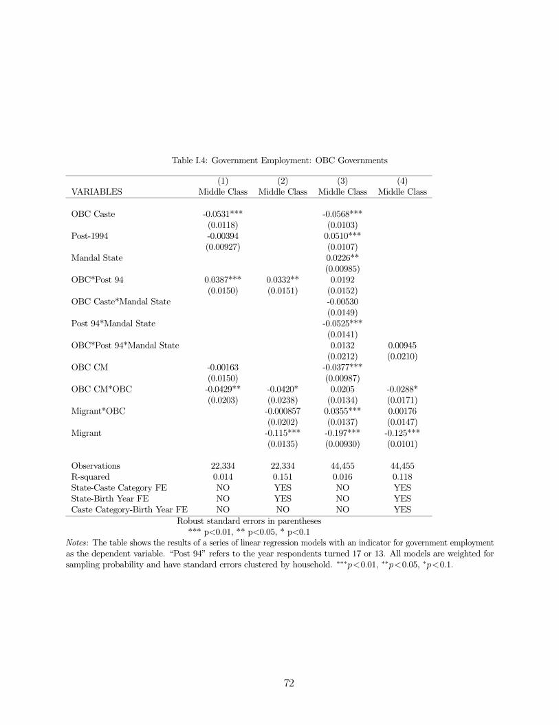
Table I.4: Government Employment: OBC Governments
(1) (2) (3) (4)VARIABLES Middle Class Middle Class Middle Class Middle Class
OBC Caste -0.0531*** -0.0568***(0.0118) (0.0103)
Post-1994 -0.00394 0.0510***(0.00927) (0.0107)
Mandal State 0.0226**(0.00985)
OBC*Post 94 0.0387*** 0.0332** 0.0192(0.0150) (0.0151) (0.0152)
OBC Caste*Mandal State -0.00530(0.0149)
Post 94*Mandal State -0.0525***(0.0141)
OBC*Post 94*Mandal State 0.0132 0.00945(0.0212) (0.0210)
OBC CM -0.00163 -0.0377***(0.0150) (0.00987)
OBC CM*OBC -0.0429** -0.0420* 0.0205 -0.0288*(0.0203) (0.0238) (0.0134) (0.0171)
Migrant*OBC -0.000857 0.0355*** 0.00176(0.0202) (0.0137) (0.0147)
Migrant -0.115*** -0.197*** -0.125***(0.0135) (0.00930) (0.0101)
Observations 22,334 22,334 44,455 44,455R-squared 0.014 0.151 0.016 0.118State-Caste Category FE NO YES NO YESState-Birth Year FE NO YES NO YESCaste Category-Birth Year FE NO NO NO YES
Robust standard errors in parentheses*** p<0.01, ** p<0.05, * p<0.1
Notes: The table shows the results of a series of linear regression models with an indicator for government employmentas the dependent variable. “Post 94” refers to the year respondents turned 17 or 13. All models are weighted forsampling probability and have standard errors clustered by household. ∗∗∗p<0.01, ∗∗p<0.05, ∗p<0.1.
72
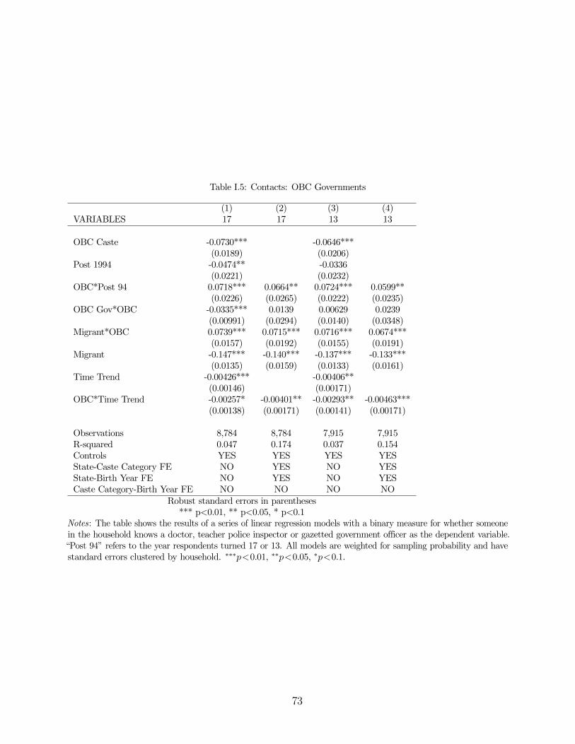
Table I.5: Contacts: OBC Governments
(1) (2) (3) (4)VARIABLES 17 17 13 13
OBC Caste -0.0730*** -0.0646***(0.0189) (0.0206)
Post 1994 -0.0474** -0.0336(0.0221) (0.0232)
OBC*Post 94 0.0718*** 0.0664** 0.0724*** 0.0599**(0.0226) (0.0265) (0.0222) (0.0235)
OBC Gov*OBC -0.0335*** 0.0139 0.00629 0.0239(0.00991) (0.0294) (0.0140) (0.0348)
Migrant*OBC 0.0739*** 0.0715*** 0.0716*** 0.0674***(0.0157) (0.0192) (0.0155) (0.0191)
Migrant -0.147*** -0.140*** -0.137*** -0.133***(0.0135) (0.0159) (0.0133) (0.0161)
Time Trend -0.00426*** -0.00406**(0.00146) (0.00171)
OBC*Time Trend -0.00257* -0.00401** -0.00293** -0.00463***(0.00138) (0.00171) (0.00141) (0.00171)
Observations 8,784 8,784 7,915 7,915R-squared 0.047 0.174 0.037 0.154Controls YES YES YES YESState-Caste Category FE NO YES NO YESState-Birth Year FE NO YES NO YESCaste Category-Birth Year FE NO NO NO NO
Robust standard errors in parentheses*** p<0.01, ** p<0.05, * p<0.1
Notes: The table shows the results of a series of linear regression models with a binary measure for whether someonein the household knows a doctor, teacher police inspector or gazetted government officer as the dependent variable.“Post 94” refers to the year respondents turned 17 or 13. All models are weighted for sampling probability and havestandard errors clustered by household. ∗∗∗p<0.01, ∗∗p<0.05, ∗p<0.1.
73


