Download - DUKE UNIVERSITY SPRING 2012
SIMPLE MODEL OF CLOSED ECONOMY
WITH THE PRESENCE OF RICARDIAN
EQUIVALENCE (Sticky Prices, Flexible Wages, Competitive Labor Market)
Prepared for Econ 296s Project
Tevy Chawwa Aditya Rachmanto
DUKE
UNIVERSITY
SPRING 2012

1
Contents
I. INTRODUCTION ............................................................................................................................... 1
II. MODEL ............................................................................................................................................ 2
A. GENERAL ASSUMPTIONS .............................................................................................................. 2
B. VARIABLES AND PARAMETERS ..................................................................................................... 2
C. BASIC EQUATIONS ....................................................................................................................... 3
III. SIMULATION RESULTS AND ANALYSIS .......................................................................................... 7
A. Policy: Increase in government expenditure ................................................................................. 7
B. Policy: Increase in income tax ...................................................................................................... 8
C. Policy: Increase in money supply .................................................................................................. 9
D. Policy: Increase in price ................................................................................................................ 9
E. Policy: Increase in Capital or Technology .................................................................................... 10
IV. CONCLUSION ............................................................................................................................. 11
APPENDIX 1 - Derivation of Differential Forms ....................................................................................... 12
APPENDIX 2 – Policy Matrices ................................................................................................................ 14
1
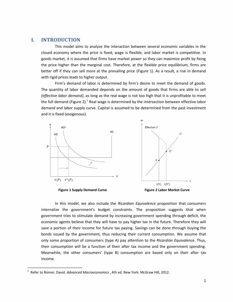
I. INTRODUCTION This model aims to analyze the interaction between several economic variables in the
closed economy where the price is fixed, wage is flexible, and labor market is competitive. In
goods market, it is assumed that firms have market power so they can maximize profit by fixing
the price higher than the marginal cost. Therefore, at the flexible price equilibrium, firms are
better off if they can sell more at the prevailing price (Figure 1). As a result, a rise in demand
with rigid prices leads to higher output.
Firm’s demand of labor is determined by firm’s desire to meet the demand of goods.
The quantity of labor demanded depends on the amount of goods that firms are able to sell
(effective labor demand), as long as the real wage is not too high that it is unprofitable to meet
the full demand (Figure 2).1 Real wage is determined by the intersection between effective labor
demand and labor supply curve. Capital is assumed to be determined from the past investment
and it is fixed (exogenous).
Figure 1 Supply Demand Curve Figure 2 Labor Market Curve
In this model, we also include the Ricardian Equivalence proposition that consumers
internalize the government's budget constraints. The proposition suggests that when
government tries to stimulate demand by increasing government spending through deficit, the
economic agents believe that they will have to pay higher tax in the future. Therefore they will
save a portion of their income for future tax paying. Savings can be done through buying the
bonds issued by the government, thus reducing their current consumption. We assume that
only some proportion of consumers (type A) pay attention to the Ricardian Equivalence. Thus,
their consumption will be a function of their after tax income and the government spending.
Meanwhile, the other consumers’ (type B) consumption are based only on their after tax
income.
1 Refer to Romer, David. Advanced Macroeconomics , 4th ed. New York: McGraw Hill, 2012.
P
Y
AD1
ADAS
LS
Effective Ld
L
w
L(Y L(Y1
E
E1

2
With the aforementioned assumptions, we will develop a model that will analyze the
impact of government spending, tax, monetary policy and price increases on output,
consumption, investment, interest rate, wage, and rental rate. There will be 3 cases: (i) 100%
type A consumers (they pay attention to Ricardian Equivalence and have smaller marginal
propensity to consume (mpc)); (ii) 50% type A consumers and 50% type B consumers (they do
not care about Ricardian Equivalence and have higher mpc); and (iii) 100% type B consumers.
In general, the result of this model conforms to the theory that the impacts of
government spending and changes in tax on all endogenous variables are smaller when more
consumers pay attention to Ricardian Equivalence and have less marginal propensity to
consume. One important difference between this model and the flexible price model is the
wage rate in this model does not depend on the marginal productivity of labor, but it depends
on the effective demand of labor. Thus, an increase in the demand of labor will increase the
wage rate. Moreover, since output is determined by demand of goods, an increase in capital or
technology will not have any impact on output. An increase in capital will only cause the
decrease in labor demand, real wage and rental rate. Meanwhile, an increase in technology will
only cause a decrease in labor demand and real wage.
II. MODEL
A. GENERAL ASSUMPTIONS
Fixed prices and fixed technological coefficient.
Labor is demand-constrained (endogenous). Labor supply is a function of real wage.
Capital is determined in the past (exogenous).
There are 2 types of consumer:
o Type A: lower mpc and pays attention to Ricardian Equivalence; and
o Type B: higher mpc and does not pay attention to Ricardian Equivalence.
If a consumer pays attention to Ricardian Equivalence, consumption is a function of mpc,
income after tax and government spending. Otherwise, it is a function of mpc and income
after tax.
B. VARIABLES AND PARAMETERS
Variables and parameters used in the model are described in Table 1 and Table 2. We use 9
endogenous variables, 6 exogenous variables and 11 parameters.

3
Table 1 Description of Variables
Table 2 Parameters
Parameters Definition Initial Value α Elasticity of output w.r.t. labor 0.7
ir Elasticity of investment w.r.t. interest rate 1
mpcA MPC for consumer type A 0.5
mpcB MPC for consumer type B 0.8
mr Elasticity of money demand w.r.t. interest rate 1
kr Elasticity of kapital w.r.t. interest rate 1
kv Elasticity of kapital w.r.t. real rate 1
θA Proportion of consumer type A Case 1: 0 Case 2: 0.5 Case 3 : 1
θB Proportion of consumer type B Case 1: 1 Case 2: 0.5 Case 3 : 0
y Initial output 100
lw Elasticity of labor supply to real wages 1
C. BASIC EQUATIONS 2
We use 9 equations to define the relationship between the variables in the economy as
follows:
1. National Accounts
Aggregate demand for a closed economy is given by dy c i g where c is aggregate
consumption, i is aggregate capital investment, and g is government purchases of goods and
2 Derivation of the equations can be seen in the Appendix
Variables Definition Unit Status
y real income widgets per year Endogenous
c real consumption widgets per year Endogenous
i real investment widgets per year Endogenous
g real gov. expenditure widgets per year Exogenous
r interest rate proportion/year Endogenous t real tax collection widgets per year Exogenous
P price level $/widget Exogenous
M money stock $ Exogenous
a Technological coefficient Unit Exogenous
w real wage widget per person year Endogenous
v real rental rate widgets per machine year Endogenous
W nominal wage $ per person year Endogenous
V nominal rental rate $ per machine year Endogenous
L Labor Workers Endogenous
K capital Machine Exogenous

4
services or government spending. The economy is in equilibrium when domestic production sy equals aggregate demand dy .
The national accounts equation can then be written as: y c i g .
The differential form of the national accounts equation is: ˆy y dc di dg .
We need the initial value of y, which we assume to be 100.
2. Consumption Function
Consumption consists of two parts: autonomous consumption and induced consumption.
(i) Autonomous consumption is the consumption that would take place if current
year’s income was zero. We assume that autonomous consumption is zero.
(ii) Induced consumption is the fraction of disposable income yD (defined as income
minus net taxes or y–t) that is used for consumption. The fraction is defined from
the parameter mpc.
The basic Keynesian consumption function can then be written as: ( )c mpc y t
We assume that there are two types of consumers, i.e., consumers who pay attention to
Ricardian Equivalence and have lower mpc (Type A); and consumers who do not pay
attention to Ricardian Equivalence and have higher mpc (Type B). Thus, we will split the
consumption function into two parts, and we can split the total real income into two, i.e.,
income for Type A consumer ( A y ) and Type B consumer ( B y ). A denotes the
proportion of Type A consumer in the population, and B the proportion for Type B
consumer.
Furthermore, since we assume the presence of Ricardian Equivalence, and that only Type A
consumer is aware of this effect, then we can formulate the disposable income as follows:
(i) Type A consumer: according to the concept of Ricardian Equivalence, when the
government increases its spending, consumers will not increase their consumption,
since they are aware that the government is financing its spending from debt, and in
the future the government will have to pay the debt by increasing tax. Hence the
consumer will save a portion of its current income to pay the future tax. One of the
means of consumer savings in the concept of Ricardian Equivalence is by buying
government bonds, which means that the consumers are financing the government
spending. For this reason, the disposable income is the fraction of total income
minus net taxes minus government spending ( )A y t g .
(ii) Type B consumer: since we assume that Type B consumer are not aware of
Ricardian Equivalence, we can formulate the disposable income as the fraction of
total income minus tax ( )B y t .
Since each type of consumers has their own mpc, we will denote Ampc for Type A
consumer, and Bmpc for Type B consumer, where we assume Ampc < Bmpc .
5
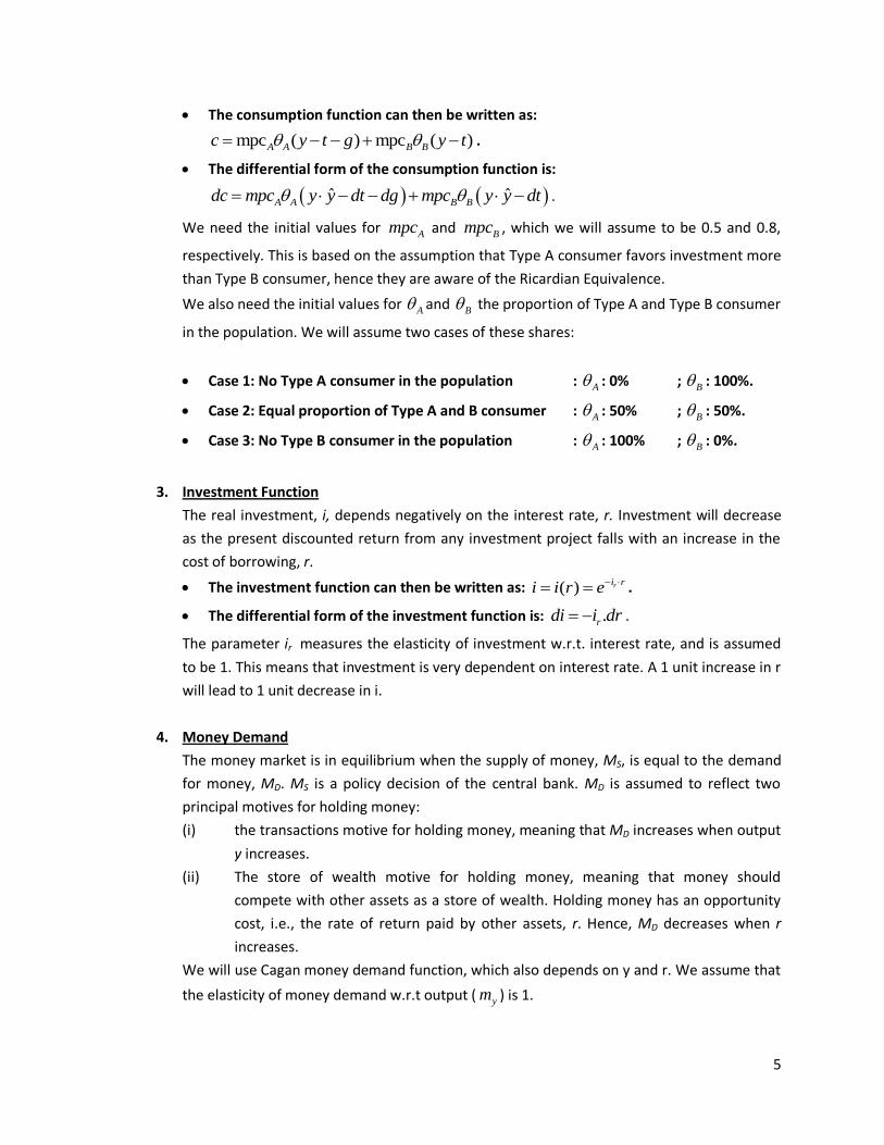
The consumption function can then be written as:
mpc ( ) mpc ( )A A B Bc y t g y t .
The differential form of the consumption function is:
ˆ ˆA A B Bdc mpc y y dt dg mpc y y dt .
We need the initial values for Ampc and
Bmpc , which we will assume to be 0.5 and 0.8,
respectively. This is based on the assumption that Type A consumer favors investment more
than Type B consumer, hence they are aware of the Ricardian Equivalence.
We also need the initial values for A and
B the proportion of Type A and Type B consumer
in the population. We will assume two cases of these shares:
Case 1: No Type A consumer in the population : A : 0% ; B : 100%.
Case 2: Equal proportion of Type A and B consumer : A : 50% ; B : 50%.
Case 3: No Type B consumer in the population : A : 100% ; B : 0%.
3. Investment Function
The real investment, i, depends negatively on the interest rate, r. Investment will decrease
as the present discounted return from any investment project falls with an increase in the
cost of borrowing, r.
The investment function can then be written as: ( ) ri ri i r e
.
The differential form of the investment function is: .rdi i dr .
The parameter ir measures the elasticity of investment w.r.t. interest rate, and is assumed
to be 1. This means that investment is very dependent on interest rate. A 1 unit increase in r
will lead to 1 unit decrease in i.
4. Money Demand
The money market is in equilibrium when the supply of money, MS, is equal to the demand
for money, MD. MS is a policy decision of the central bank. MD is assumed to reflect two
principal motives for holding money:
(i) the transactions motive for holding money, meaning that MD increases when output
y increases.
(ii) The store of wealth motive for holding money, meaning that money should
compete with other assets as a store of wealth. Holding money has an opportunity
cost, i.e., the rate of return paid by other assets, r. Hence, MD decreases when r
increases.
We will use Cagan money demand function, which also depends on y and r. We assume that
the elasticity of money demand w.r.t output ( ym ) is 1.

6
The money demand function can then be written as: ( , ) y rm m rM
f y r y eP
.
The differential form of the money demand is:
ˆ ˆ ˆrM P y m dr
The parameter mr measures the elasticity of money demand w.r.t. interest rate, and is
assumed to be 1. This means that money demand is very dependent on interest rate.
5. Production Function
Production is assumed to be a Cobb-Douglas function with two factor inputs, capital and
labor, and a technological coefficient.
The production function can then be written as: 1y aK L .
The differential form of the production function is:
ˆ ˆˆ ˆ (1 )y a K L
The parameter α measures the elasticity of output w.r.t. labor, and is assumed to be 0.7.
This means that elasticity of output w.r.t. capital is 0.3.
6. Labor Supply
Since labor is endogenous, then the amount of effective labor force is determined from the
intersection between labor supply (LS) curve and labor demand (LD) curve in the equilibrium.
LD is determined from the production function. LS is a function of the real wage. If real wage
increases, then labor supply will increase.
It is worth noting that the equilibrium real wage is not the marginal product of labor
anymore, since real wage is now a function of LS.
The labor supply function can then be written as: wlW
L f f w wP
.
The differential form of the labor supply is: ˆ ˆwL l w .
The parameter lw measures the elasticity of labor force w.r.t. real wage, and is assumed to
be 1.
7. Nominal Wage
Nominal wage is the dollar value of real wage, which is defined as the product of real wage
and price.
The nominal wage function can then be written as: W w P .
The differential form of the nominal wage is:
ˆ ˆˆW w P .
8. Real Rental Rate
Real wage is defined as the marginal product of capital (MPK) from the Cobb-Douglas
production function.
7
The real rental rate function can then be written as: (1 )y
v a K LK
.
The differential form of the real rental rate is:
ˆ ˆˆ ˆ ( )v a K L .
9. Nominal Rental Rate
Nominal rental rate is the dollar value of real rental rate, which is defined as the product of
real rental rate and price.
The nominal rental rate function can then be written as: V v P .
The differential form of the nominal rental rate is:
ˆ ˆˆV v P .
III. SIMULATION RESULTS AND ANALYSIS
A. Policy: Increase in government expenditure
The effect of 1 % increase in government expenditure for each case is presented in
Figure 3. In general, this policy will increase output, consumption, labor, real and nominal wage
rate, interest rate, real and nominal rental rate. Furthermore, the increase in interest rate will
decrease investment which popularly called as crowding out effect. In line with theory, the
effect of this policy on economy is smaller when more people pay attention to Ricardian
equivalence proposition.
Figure 3 Impact of Increase in Government Expenditure Note: For graphs purposes, due to the high values of dc, it is calibrated so that dc = dc / y = dc / 100
Explanations:
Increase in government expenditure will increase the aggregate demand. Therefore, at fixed
price, firms will increase their output to meet the demand. To produce more output, firms need
more labor, then the demand of effective labor L^ increases. Since sensitivity of labor supply
with respect to real wage = 1, then the real wages (when labor demand meets labor supply)
increases. Since price is fixed, the nominal wage W increases.
The increase in total output y^ makes the quantity of money demanded increases. Holding
M and P constant, interest rate must increases to compensate the excess demand of money.
-0.060
-0.040
-0.020
0.000
0.020
0.040
0.060
0.080
y^ dc di L^ dr W^ w^ v^ V^
A= 0%; B= 100% A=50%; B=50% A=100%; B= 0%
A= 0%; B= 100% A=50%; B=50% A=100%; B= 0%
y 0.0476 0.0208 0.0098
dc 3.810 1.104 -0.010
di -0.048 -0.021 -0.010
L^ 0.068 0.030 0.014
dr 0.048 0.021 0.010
W^ 0.068 0.030 0.014
w^ 0.068 0.030 0.014
v^ 0.048 0.021 0.010
V^ 0.048 0.021 0.010
8
The increase in interest rate makes investment spending decrease. The decrease in investment
causes by the increase of government spending explains the crowding out effect.
Since real rental rate is defined as the marginal product of capital and capital is
constant, then increase in output makes real rental rate increases. Holding P constant, the
nominal rental rate must increase.
Increase in output can be seen as increase in income, therefore normally consumption
should be increase. However, since consumers type A believe of ricardian equivalence then they
will decrease their consumption. Aggregately when proportion of consumer type A increase,
then the impact of government spending on consumption will be less and could be negative
(case 3).
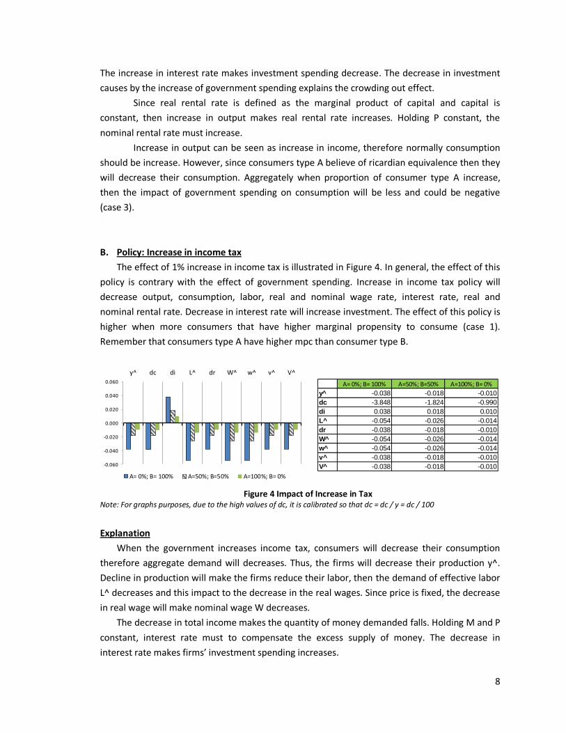
B. Policy: Increase in income tax
The effect of 1% increase in income tax is illustrated in Figure 4. In general, the effect of this
policy is contrary with the effect of government spending. Increase in income tax policy will
decrease output, consumption, labor, real and nominal wage rate, interest rate, real and
nominal rental rate. Decrease in interest rate will increase investment. The effect of this policy is
higher when more consumers that have higher marginal propensity to consume (case 1).
Remember that consumers type A have higher mpc than consumer type B.
Figure 4 Impact of Increase in Tax Note: For graphs purposes, due to the high values of dc, it is calibrated so that dc = dc / y = dc / 100
Explanation
When the government increases income tax, consumers will decrease their consumption
therefore aggregate demand will decreases. Thus, the firms will decrease their production y^.
Decline in production will make the firms reduce their labor, then the demand of effective labor
L^ decreases and this impact to the decrease in the real wages. Since price is fixed, the decrease
in real wage will make nominal wage W decreases.
The decrease in total income makes the quantity of money demanded falls. Holding M and P
constant, interest rate must to compensate the excess supply of money. The decrease in
interest rate makes firms’ investment spending increases.
-0.060
-0.040
-0.020
0.000
0.020
0.040
0.060
y^ dc di L^ dr W^ w^ v^ V^
A= 0%; B= 100% A=50%; B=50% A=100%; B= 0%
A= 0%; B= 100% A=50%; B=50% A=100%; B= 0%
y -0.038 -0.018 -0.010
dc -3.848 -1.824 -0.990
di 0.038 0.018 0.010
L^ -0.054 -0.026 -0.014
dr -0.038 -0.018 -0.010
W^ -0.054 -0.026 -0.014
w^ -0.054 -0.026 -0.014
v^ -0.038 -0.018 -0.010
V^ -0.038 -0.018 -0.010

9
Since capital is constant and output decrease, the marginal product of capital or real rental
rate will decreases. Holding P constant, the nominal rental rate must decreases.
C. Policy: Increase in money supply
The effect of 1 % in money supply is illustrated in Figure 5. In general, this policy will
increase output, consumption, investment, labor, real and nominal wage, real and nominal
rental rate. Furthermore, it will decrease interest rate. The impact of monetary policy on output
and consumption the effect of monetary policy is higher when more consumers have higher
marginal propensity to consume (case 1).
Figure 5 Impact of Increase in Money Supply Note: For graphs purposes, due to the high values of dc, di and dr, it is calibrated so that dc=dc/100, di=di/10
and dr= dr/10
Explanation
1% increase in money supply will decrease the interest rate and increase aggregate
demand. The increase in aggregate demand will make the firms increase their production. The
decreases in interest rate make firms’ investment spending increases.
Increase in production will make the firms add more labor, then the demand of effective
labor increases and this impact to the increase in the real wages. Since price is fixed, the inrease
in real wage will make nominal wage W increases.
Since the capital is constant, then increase in the output will increase the marginal
product of capital or real rental rate. Holding P constant, the nominal rental rate must increase.
Increase in output can be seen as increase in income, therefore consumption will be
increase. When consumers type A (higher mpc) is more dominant, the effect of monetary policy
is higher.
D. Policy: Increase in price
Suppose the firms want a higher profit and they increase price by 1%. The effect of this
action is illustrated in figure 6. In general, this policy will decrease output, consumption,
investment, labor, real wage and real rental rate. Furthermore, it will increase interest rate,
nominal wage and nominal rental rate of capital. The impact of price on output and
-0.150
-0.100
-0.050
0.000
0.050
0.100
0.150
y^ dc di L^ dr W^ w^ v^ V^
A= 0%; B= 100% A=50%; B=50% A=100%; B= 0%
A= 0%; B= 100% A=50%; B=50% A=100%; B= 0%
y 0.048 0.028 0.020
dc 3.810 1.806 0.980
di 0.952 0.972 0.980
L^ 0.068 0.040 0.028
dr -0.952 -0.972 -0.980
W^ 0.068 0.040 0.028
w^ 0.068 0.040 0.028
v^ 0.048 0.028 0.020
V^ 0.048 0.028 0.020

10
consumption is higher when more consumers have higher marginal propensity to consume (case
1)
Figure 6 Impact of Increase in Price Note: For graphs purposes, due to the high values of dc, di, dr,W^ and V^ it is calibrated
so that dc=dc/100, di=di/10, dr= dr/10, W^=W^/10 and V^=V^/10
Explanation
Increase in price will decrease aggregate demand and increase the interest rate. The
decrease in aggregate demand will make the firms decrease their production. The increases in
interest rate make firms’ investment spending decreases. Decrease in output can be seen as
decrease of income, therefore consumption will decrease.
Lower production will make the firms reduce labor, then the demand of effective labor
decreases and this impact to the decrease in the real wages. Since price is increase higher than
the decrease in real wage, the nominal wage W will increases.
Since the capital is constant meanwhile output decrease, then the marginal product of
capital will decrease and real rental rate decreases.
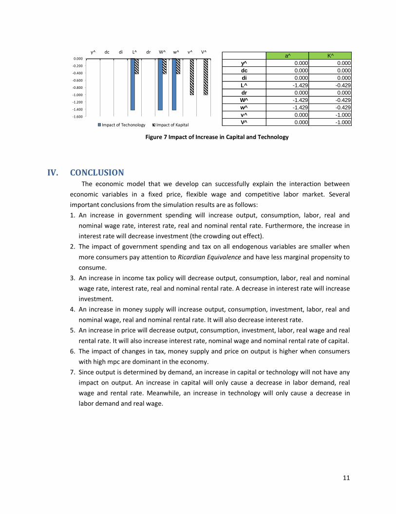
E. Policy: Increase in Capital or Technology
Increase in capital or technology will not have impact to output, since output is demand-
constrained. Therefore, changes in those variable wouldn’t impact consumption, investment
and interest rate. Increase in capital and technology will make the demand of labor decrease,
because number of output is constant. Therefore labor and real wage will decrease. On the
other side, increase in capital will decrease the rental rate. Since price is constant, then nominal
wage and nominal rental rate will decrease. The impact of 1% increase in capital and 1%
increase in technology can be seen in Figure 8.
-0.150
-0.100
-0.050
0.000
0.050
0.100
0.150
y^ dc di L^ dr W^ w^ v^ V^
A= 0%; B= 100% A=50%; B=50% A=100%; B= 0%
A= 0%; B= 100% A=50%; B=50% A=100%; B= 0%
y -0.048 -0.028 -0.020
dc -3.810 -1.806 -0.980
di -0.952 -0.972 -0.980
L^ -0.068 -0.040 -0.028
dr 0.952 0.972 0.980
W^ 0.932 0.960 0.972
w^ -0.068 -0.040 -0.028
v^ -0.048 -0.028 -0.020
V^ 0.952 0.972 0.980
11
Figure 7 Impact of Increase in Capital and Technology
IV. CONCLUSION The economic model that we develop can successfully explain the interaction between
economic variables in a fixed price, flexible wage and competitive labor market. Several
important conclusions from the simulation results are as follows:
1. An increase in government spending will increase output, consumption, labor, real and
nominal wage rate, interest rate, real and nominal rental rate. Furthermore, the increase in
interest rate will decrease investment (the crowding out effect).
2. The impact of government spending and tax on all endogenous variables are smaller when
more consumers pay attention to Ricardian Equivalence and have less marginal propensity to
consume.
3. An increase in income tax policy will decrease output, consumption, labor, real and nominal
wage rate, interest rate, real and nominal rental rate. A decrease in interest rate will increase
investment.
4. An increase in money supply will increase output, consumption, investment, labor, real and
nominal wage, real and nominal rental rate. It will also decrease interest rate.
5. An increase in price will decrease output, consumption, investment, labor, real wage and real
rental rate. It will also increase interest rate, nominal wage and nominal rental rate of capital.
6. The impact of changes in tax, money supply and price on output is higher when consumers
with high mpc are dominant in the economy.
7. Since output is determined by demand, an increase in capital or technology will not have any
impact on output. An increase in capital will only cause a decrease in labor demand, real
wage and rental rate. Meanwhile, an increase in technology will only cause a decrease in
labor demand and real wage.
-1.600
-1.400
-1.200
-1.000
-0.800
-0.600
-0.400
-0.200
0.000
y^ dc di L^ dr W^ w^ v^ V^
Impact of Techonology Impact of Kapital
a^ K^
y 0.000 0.000
dc 0.000 0.000
di 0.000 0.000
L^ -1.429 -0.429
dr 0.000 0.000
W^ -1.429 -0.429
w^ -1.429 -0.429
v^ 0.000 -1.000
V^ 0.000 -1.000

12
APPENDIX 1 - Derivation of Differential Forms
1. National Accounts
ˆ.
y c i g
y y y ydy dc di dg
y c i g
y y dc di dg
2. Consumption function
mpc ( ) mpc ( )
ˆ
ˆ
A A B B
A A
B B
A A
B B
A A
B B
c y t g y t
c c cdc mpc dy dt dg
y t g
c cmpc dy dt
y t
mpc dy dt dg
mpc dy dt
dc mpc y y dt dg
mpc y y dt
3. Investment function
.
r
r
r
i r
i r
r
i r
r
i i r e
idi dr
r
i e drdi
i e
di i dr
4. Money demand
1
( , )
Let : equals 1, then
ˆ ˆ ˆ
y r
y r
y y yr r r
y r
m m r
m m r
m m mm r m r m r
y r
m m r
y r
y
r
Mf y r y e
P
M Py e
M M MdM dP dy dr
P y r
y e dP m Py e dy m Py e drdM
M Py e
dP dym m dr
P y
m
M P y m dr
5. Production function 1
1
1 1
(1 )
(1 )
ˆ ˆˆ ˆ (1 )
y aK L
y y ydy da dK dL
a K L
K L da a K L dK
a K L dL
dy da dK dL
y a K L
y a K L
6. Labor Supply
1
1
ˆ ˆ
w
w
w
w
l
l
w
l
w
l
w
WL f f w w
P
dL l w dw
l w dwdL
L w
L l w

13
7. Nominal wage
ˆ ˆˆ
W w P
W WdW dw dP
w P
dW dw dP
W w P
W w P
8. Real rental rate
1
1
(1 )
(1 ) (1 )
(1 )
ˆ ˆˆ ˆ ( )
yv a K L
K
v v vdv da dK dL
a K L
K L da a K L dK
a K L dL
dv da dK dL
v a K L
v a K L
9. Nominal rental rate
ˆ ˆˆ
V v P
V VdV dv dP
v P
dV dv dP
V w P
V v P

14
APPENDIX 2 – Policy Matrices
Proportion of consumer type A = 0%, B=100%
dg dt M^ P^ a^ K^
y^ 0.048 -0.038 0.048 -0.048 0.000 0.000
dc 3.810 -3.848 3.810 -3.810 0.000 0.000
di -0.048 0.038 0.952 -0.952 0.000 0.000
L^ 0.068 -0.054 0.068 -0.068 -1.429 -0.429
dr 0.048 -0.038 -0.952 0.952 0.000 0.000
W^ 0.068 -0.054 0.068 0.932 -1.429 -0.429
w^ 0.068 -0.054 0.068 -0.068 -1.429 -0.429
v^ 0.048 -0.038 0.048 -0.048 0.000 -1.000
V^ 0.048 -0.038 0.048 0.952 0.000 -1.000
Proportion of consumer type A = 50%, B=50%
dg dt M^ P^ a^ K^
y^ 0.021 -0.018 0.028 -0.028 0.000 0.000
dc 1.104 -1.824 1.806 -1.806 0.000 0.000
di -0.021 0.018 0.972 -0.972 0.000 0.000
L^ 0.030 -0.026 0.040 -0.040 -1.429 -0.429
dr 0.021 -0.018 -0.972 0.972 0.000 0.000
W^ 0.030 -0.026 0.040 0.960 -1.429 -0.429
w^ 0.030 -0.026 0.040 -0.040 -1.429 -0.429
v^ 0.021 -0.018 0.028 -0.028 0.000 -1.000
V^ 0.021 -0.018 0.028 0.972 0.000 -1.000
Proportion of consumer type A = 100%, B=0%
dg dt M^ P^ a^ K^
y^ 0.0098 -0.010 0.020 -0.020 0.000 0.000
dc -0.010 -0.990 0.980 -0.980 0.000 0.000
di -0.010 0.010 0.980 -0.980 0.000 0.000
L^ 0.014 -0.014 0.028 -0.028 -1.429 -0.429
dr 0.010 -0.010 -0.980 0.980 0.000 0.000
W^ 0.014 -0.014 0.028 0.972 -1.429 -0.429
w^ 0.014 -0.014 0.028 -0.028 -1.429 -0.429
v^ 0.010 -0.010 0.020 -0.020 0.000 -1.000
V^ 0.010 -0.010 0.020 0.980 0.000 -1.000


