
DV3+HED+: A DCNNs-based Framework to
Monitor Temporary Works and ESAs in Railway
Construction Project Using VHR Satellite Images
Rui Guo1,2, Ronghua Liu4, Na Li 3, * Wei Liu1,2
1 Aerospace Information Research Institute, Chinese Academy of Sciences, No.9 Dengzhuang South
Road, Haidian District, Beijing, P.R. China 100094, [email protected] (R. G.); [email protected]
(W. L.);
2 Institute of Remote Sensing and Digital Earth, Chinese Academy of Sciences, No.9 Dengzhuang
South Road, Haidian District, Beijing, P.R. China 100094.
3 Ping An Technology (Shenzhen) Co., Ltd, Shenzhen, P.R. China 200240; [email protected].
4 China Institute of Water Resources and Hydropower Research, Beijing, P.R. China 100038,
* Correspondence: [email protected]; Tel.: +86-10-8217-8151
Received: date; Accepted: date; Published: date
Abstract: Current VHR(Very High Resolution) satellite images enable the detailed
monitoring of the earth and can capture the ongoing works of railway construction. In this
paper, we present an integrated framework applied to monitoring the railway construction in
China, using QuickBird, GF-2 and Google Earth VHR satellite images. We also construct a
novel DCNNs-based (Deep Convolutional Neural Networks) semantic segmentation network
to label the temporary works such as borrow & spoil area, camp, beam yard and
ESAs(Environmental Sensitive Areas) such as resident houses throughout the whole railway
construction project using VHR satellite images. In addition, we employ HED edge detection
sub-network to refine the boundary details and attention cross entropy loss function to fit the
sample class disequilibrium problem. Our semantic segmentation network is trained on 572
VHR true color images, and tested on the 15 QuickBird true color images along Ruichang-
Jiujiang railway during 2015-2017. The experiment results show that compared with the
existing state-of-the-art approach, our approach has obvious improvements with an overall
accuracy of more than 80%.
Keywords: railway construction; deep learning; remote sensing; convolution neural network;
semantic segmentation
1. Introduction
Railways have been vital in supporting the society, people’s livelihood and economic
development in China over the past 40 years. The rapid development of the railway
construction provides convenient transportation for people and accelerates economic and
social development, but it occupies and destroys a certain amount of land resources inevitably
as well. How to control and reduce the negative effects to environment brought by railway
construction has become a key issue that both the administrative management and project
construction department must confront and resolve.
The environment monitoring during railway construction project is to supervise and
inspect the execution of environmental protection measures on the basis of the design and
environment evaluation report of this project and to affirm the achievements, find out existing
problems and give suggestions on countermeasures. According to the different functions, the

construction project of railway consists of three parts, which are permanent works, temporary
works and ESAs. The permanent works mainly contain roadbeds, tracks, stations, bridges,
piers, culverts, water supply and sewerage work, and electrification facilities etc., which should
be strictly checked and accepted according to the project plan during the construction. The
temporary works mainly contain borrow areas, spoil areas, camps and beam yards which play
a distinctly subsidiary role but have significant influences to the environment during the
project construction. The ESAs mainly refer to resident houses which concern with the critical
relocation affairs of nearby residents. In this paper, we mainly focus on the monitoring of
temporary works and ESAs, which are illustrated in Table 1.
Table 1. Description of temporary works and ESAs
Construction name Construction
type
Geometory
type Description
Borrow area Temporary work Polygon
An area designated as the excavation
site for geologic resources, such as
rock/basalt, sand, gravel, or soil.
Spoil area Temporary work Polygon
An area used to refer to material
removed when digging a foundation,
tunnel, or other large excavation.
Resident house ESA Polygon
Residents within 30 meters apart
from the boundary of the land used
by the project should be relocated.
Camp Temporary work Polygon Camp for workers.
Beam yard Temporary work Polygon -
As long linear construction projects, many railways go through regions of complex terrain,
which poses great difficulties to monitoring current status of temporary works and ESAs. With
the advantages of low cost, periodic data acquiring, and historical data archiving, VHR satellite
images are very suitable for monitoring the changes along the railway. Pixel-wise classification
such as support vector machines[1], neural networks[2], random forest[3] are widely used to
classify low spatial resolution (10–30m) images. In the past 10 years, GEOBIA(Geographic
Object-Based Image Analysis) has been explored to deal with high spatial variability in the
VHR images[4]. However, the performance of GEOBIA is inherently dependent on the level of
the segmentation results. Considering the complexity of land cover that contains vegetation,
water, soil and other physical land features, it is still challenging for GEOBIA to improve
classification accuracy in VHR images.
From the other perspective, traditional pixel-wise classification and GEOBIA focused
feature extraction approaches such as SIFT(Scale-Invariant Feature Transform)[5] and
HOG(Histogram of Oriented Gradient)[6] and supervised learning algorithms. However, the
two steps mentioned above are typically treated as independent approaches. DCNNs fuse the
them into one network that learns semantic features at different scales and computes the score
of each class at the end of the network. In recent years, DCNNs have performed quite well in
computer vision tasks, such as image classification, targets detection and semantic
segmentation.
In this paper, we present a novel framework for temporary works and ESAs monitoring
of railway construction project using VHR satellite images. Compared to existing studies, our
novel contributions are as follows:
We construct a novel workflow for temporary works and ESAs monitoring of railway
construction project using VHR satellite images.

We construct an efficient supervised learning model for VHR images classification based
on the fusion of the state of art semantic segmentation network DV3+(DeepLabV3 plus)[7]
and HED (Holistically-nested Edge Detection)[8].
For the sake of solving class imbalance problem of training data, we introduce attention
loss function to the ground object boundary detection in HED.
2. Related work
According to the published studies, satellite remote sensing has not been used in
temporary works or ESAs monitoring for railway construction project. However, satellite
images had been used for monitoring the changes of light rail transport construction in Kuala
Lumpur, Malaysia[9]. Likewise, Giannico[10] present site detection and EIA(Environmental
Impact Assessment) method due to the construction using satellite images. Lin[11] employed
UAV to monitor abandoned dreg fields of high-speed railway construction. Chang[12] detected
the railway subsidiaries using interferometric synthetic aperture radar techniques. Arastounia[13]
presented an automated recognition method of railroad infrastructure in rural areas using LIDAR
data.
Over the last few years, methods based on FCNs(Fully Convolutional Networks) [14] have
demonstrated significant improvement on PASCAL15] and MS-COCO [16] segmentation
benchmarks than the traditional pixel-wise classification and GEOBIA. SegNet[17] introduced
an encoder and decoder network into the pooling indices. U-Net[18] adds skip connections from
the encoder features to the corresponding decoder activations. RefineNet[19] combined rough
high-level semantic features and fine-grained low-level features. Inspired by SegNet and
ResNet[20], LinkNet[21] introduced residual blocks to the network architecture, which made
efficient use of scarce resources available on embedded platforms without any significant
increase in number of parameters. PSPNet[22] concatenated the regular CNN layers and the
upsampled pyramid pooling layers, carrying both local and global context information to the
image. BiSeNet[23] designed spatial path and context path, and tried to use a new method to
keep both spatial context and spatial detail at the same time. The Deeplab series which contains
LargeFOV(DeepLab Large Field-Of-View)[24], ASPP(DeepLab Atrous Spatial Pyramid
Pooling)[25], DV3(Deeplab V3)[26] and DV3+[7] employed atrous convolution, fully connected
CRFs to localize the segment boundaries and encoder-decoder framework achieved a higher
accuracy than previous methods.
In remote sensing research, Penatti[27] showed that a pre-trained CNN used to recognize
natural image objects generalizes well to remote sensing images by transfer learning. Based on
FCN, many frameworks were derived to learn features at different scales and fusing such features
in many ways[28,29,30,31]. Marmanis[32] extracted scale-dependent class boundaries before each
pooling level, with the class boundaries fused into the final multi-scale boundary prediction. Guo
[33] extracted bounding boxes of potential ground objects which augmented the training dataset
before training the DCNNs. Tian[34] presented DFCNet(Dense Fusion Classmate Network)
which was jointly trained with auxiliary road dataset properly compensates the lack of mid-level
information. Li[35] proposed Y-Net which contained a two-arm feature extraction module and a
fusion module for road segmentation.
Nevertheless, the tendency of the DCNNs is to extract and fuse the global semantic
features and local features from different scales.
3. Satellite data collection and processing
3.1. Satellite data collection
As deep learning is a data-driven method, DCNNs rely on diversity and quality of the
datasets to achieve a satisfactory training accuracy and capability of generalization. Therefore,
label data making for temporary works and ESAs became a critical task in the whole framework.
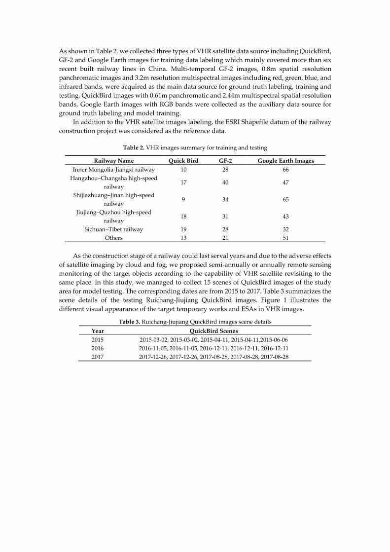
As shown in Table 2, we collected three types of VHR satellite data source including QuickBird,
GF-2 and Google Earth images for training data labeling which mainly covered more than six
recent built railway lines in China. Multi-temporal GF-2 images, 0.8m spatial resolution
panchromatic images and 3.2m resolution multispectral images including red, green, blue, and
infrared bands, were acquired as the main data source for ground truth labeling, training and
testing. QuickBird images with 0.61m panchromatic and 2.44m multispectral spatial resolution
bands, Google Earth images with RGB bands were collected as the auxiliary data source for
ground truth labeling and model training.
In addition to the VHR satellite images labeling, the ESRI Shapefile datum of the railway
construction project was considered as the reference data.
Table 2. VHR images summary for training and testing
Railway Name Quick Bird GF-2 Google Earth Images
Inner Mongolia-Jiangxi railway 10 28 66
Hangzhou–Changsha high-speed
railway 17 40 47
Shijiazhuang–Jinan high-speed
railway 9 34 65
Jiujiang–Quzhou high-speed
railway 18 31 43
Sichuan–Tibet railway 19 28 32
Others 13 21 51
As the construction stage of a railway could last serval years and due to the adverse effects
of satellite imaging by cloud and fog, we proposed semi-annually or annually remote sensing
monitoring of the target objects according to the capability of VHR satellite revisiting to the
same place. In this study, we managed to collect 15 scenes of QuickBird images of the study
area for model testing. The corresponding dates are from 2015 to 2017. Table 3 summarizes the
scene details of the testing Ruichang-Jiujiang QuickBird images. Figure 1 illustrates the
different visual appearance of the target temporary works and ESAs in VHR images.
Table 3. Ruichang-Jiujiang QuickBird images scene details
Year QuickBird Scenes
2015 2015-03-02, 2015-03-02, 2015-04-11, 2015-04-11,2015-06-06
2016 2016-11-05, 2016-11-05, 2016-12-11, 2016-12-11, 2016-12-11
2017 2017-12-26, 2017-12-26, 2017-08-28, 2017-08-28, 2017-08-28

Resident houseCamp
Beam yardBorrow area
Spoil area
Figure 1. Visual appearance of the target temporary works and ESAs in VHR images
3.2. Data processing and labeling
Time series of QuickBird, GF-2 and Google Earth satellite images were used for training
and testing in this study. The data processing workflow was shown in Figure 2. First,
panchromatic and multispectral bands of QuickBird and GF-2 images were geometrically
corrected as well as orthorectified. Then, we employed pansharpening method which
combined the high resolution of panchromatic images with the lower resolution of
multispectral ones. The advantage of such method is to get as a final result a colored image of
a certain area with a high resolution, optimizing the starting panchromatic one. Last, we mosaic
the VHR images with the same imaging time in the same railway construction project.
Moreover, the histograms of the images were adjusted to enhance the contrast. We also
employed the Google Earth RGB images as the additional data source. We search the locations
of railway construction line according to its coordinates and exported the images from the
Google Earth software. All processing for this study was completed using ArcGIS 10.4.1 by
ESRI ©. Table 4 illustrates the ground truth sample count of target temporary works and ESAs
Google Earth Images
GF-2
QuickBird
Georeferencing
Orthorectification Image Fusion
MosaicingESAs Dataset
Labeling
Images
Ground Truth
TransformationAugmentation
Object ProposalAugmentation
Data Source Data ProcessingData Augmentation
Figure 2. Data processing workflow
Table 4. Ground truth sample count of target temporary works and ESAs
Name Ground Truth Count Type
Borrow area 106 ESA
Spoil area 294 ESA
Resident houses 1953 ESA

Camp 484 Temporary work
Beam yard 25 ESA
Data augmentation has been widely used for avoiding overfitting when training data are
not sufficient to learn a generalizable model. In this paper, we followed the satellite data
augmentation method presented by Guo[42], in which the selective search method was applied
to generate bounding boxes of potential ground objects in the VHR satellite images. Thus, we
obtain more valuable trained data by using unsupervised methods than simple transformation
augmentation.
4. Methodology
DCNNs-based models and atrous convolution have proven to be the most successful
methods of semantic segmentation. The VHR remote sensing images contain abundant
geometric information of the ground object. In order to make better use of this information, we
combine the HED boundary detection network[8] and the state-of-the-art DV3+[7] semantic
segmentation network ;which integrated the advantages of ASPP and encoder-decoder for
pixel-wise classification of remote sensing imagery. In addition, we employ the Attention
Loss[36] to scale class-balanced cross entropy loss and upgrade the loss contribution of both
false negative and false positive samples during the training process.
4.1. Network architecture
Our network architecture shown in Figure 5 follows the idea of Marmanis[32], which
combines ground object boundary detection along with semantic segmentation. Based on
VGG-16, the HED outputs a multi-scale feature map before each pooling layer for edge
detection. The multi-scale feature maps are then fused into a final boundary feature map. The
relation of each scale layer loss function and fusion layer loss function is illustrated as following:
����� = � �����(�)
�
���
(1)
where �����(�)
denotes the different scale level loss function for each side output, ����� denotes fusion layer loss function of the side outputs.
After boundary detection sub-network, the network fuses the original input image and
the boundary prediction result and then the fusion of image and boundary are put into the
DV3+ semantic segmentation sub-network. The DV3+ proposes a state-of-the-art encoder-
decoder structure which employs DV3 as encoder module and a simple yet effective decoder
module for natural image semantic segmentation. The DV3+ also adapts the Xception model
and apply depth wise separable convolution to both encoder and decoder module, resulting in
a faster and stronger network. After the processing of HED and DV3+ sub-networks, the
classification results are predicted.
Due to the complexity of the ground objects and the artificial workload, we didn’t label
the boundary ground truth data for training manually. Considering that each ground object in
label data represents a different class, the edge between different classes can be regarded as the
boundary ground truth which can be produced by label data simply. In this paper, we use
Sobel edge detection operator to generate the boundary ground truth data.
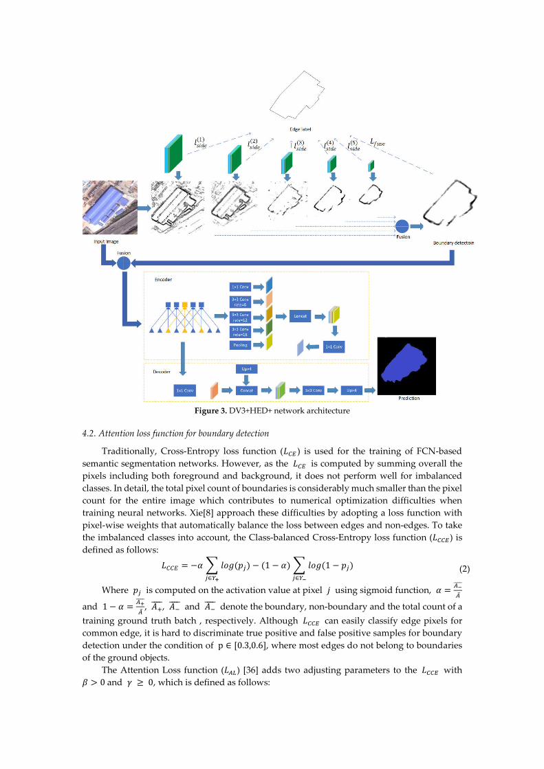
Figure 3. DV3+HED+ network architecture
4.2. Attention loss function for boundary detection
Traditionally, Cross-Entropy loss function (��� ) is used for the training of FCN-based
semantic segmentation networks. However, as the ��� is computed by summing overall the
pixels including both foreground and background, it does not perform well for imbalanced
classes. In detail, the total pixel count of boundaries is considerably much smaller than the pixel
count for the entire image which contributes to numerical optimization difficulties when
training neural networks. Xie[8] approach these difficulties by adopting a loss function with
pixel-wise weights that automatically balance the loss between edges and non-edges. To take
the imbalanced classes into account, the Class-balanced Cross-Entropy loss function (����) is
defined as follows:
���� = −� � ��� (��) − (1 − �) � ��� (1 − ��)
�∈���∈��
(2)
Where �� is computed on the activation value at pixel � using sigmoid function, � =������
�̅
and 1 − � =������
�̅, ��
����, ������ and ��
���� denote the boundary, non-boundary and the total count of a
training ground truth batch , respectively. Although ���� can easily classify edge pixels for
common edge, it is hard to discriminate true positive and false positive samples for boundary
detection under the condition of p ∈ [0.3,0.6], where most edges do not belong to boundaries
of the ground objects.
The Attention Loss function (���) [36] adds two adjusting parameters to the ���� with
� > 0 and � ≥ 0, which is defined as follows:
��� = − � ��(����)�log (��) − � (1 − �)���
�log (��)
�∈���∈��
(3)
The parameter � adjusts true positive and false positive loss contributions. The ���
penalizes misclassified samples strongly and penalizes the correctly classified samples weakly,
which is more discriminating. The parameter � smoothly accommodate the loss on the
condition of certain � value.
5. Experiment and results
In this section, we describe the training settings of the experiment and present numerical
and visual results. Meanwhile, we evaluate the benefits of each component of our proposed
method.
5.1. Training
In this paper, the experiments we have done were based on the TensorFlow framework
developed by Google and performed on a computer running the Ubuntu 16.04 operating
system and equipped with two NVIDIA RTX 2080 Ti graphics card with 22 GB of memory.
TensorFlow has been used extensively in the area of deep learning, and there are many pre-
trained models that are based on it. We could finetune the models that have been validated
successfully in natural image semantic segmentation.
The DCNNs-based model was trained by SGD (Stochastic Gradient Descent). To fit the
model, we tiled the original images into patches of 513×513 sizes supplemented with the
augmentation patches mentioned in 3.2. In every iteration, a mini-batch of patches was fed to
the n for backpropagation. In all cases, a momentum of 0.9 and an L2 penalty on the network’s
weight decay of 0.0002 were used. The learning rate was computed dynamically between 0.007
and 1e-6. Weights were initialized following [20,37], and training ended after 50,000 iterations,
when the error stabilized on the validation set.
5.2. Classification results
We evaluate the performance of our method based on three criteria: per-class accuracy,
the overall accuracy and the average recall. The accuracy is defined as the number of true
positives (��) divided by the sum of the number of true positives and the number of false
positives (��):
�������� =��
�� + �� (4)
Recall is defined as the number of true positives (��), divided by the sum of the number
of true positives and the number of false negatives (��):
������ =��
�� + �� (5)
According to the presented classification workflow and network architecture, we inferred
the 2km buffer VHR satellite images along the Ruichang-Jiujiang Railway line during 2015-
2017 based on the trained model. The classification results are shown in Table 5.

Table 5. Temporary works and ESAs classification results of Ruichang-Jiujiang railway
during 2015-2017
Year Method Borrow-spoil
area
Resident
house Camp Beam yard
Average
Recall
Overall
Accuracy
2015
DV3+ 78.52 74.37 81.42 70.84 77.17 77.23
DV3+HED 79.73 76.01 83.94 71.54 79.32 79.94
DV3+HED+ 80.91 76.56 84.33 73.18 79.87 80.05
2016
DV3+ 79.72 74.02 82.05 69.44 76.02 76.95
DV3+HED 80.3 75.87 83.84 71.03 78.41 78.72
DV3+HED+ 81.46 76.59 83.91 72.79 79.18 80.35
2017
DV3+ 78.28 75.55 82.96 65.82 77.3 78.24
DV3+HED 79.77 76.43 84.21 68.66 78.47 79.11
DV3+HED+ 80.53 76.87 84.73 69.14 78.53 80.19
The visual classification results are shown in Figure 6. From the perspective of target object
characteristics, camps, borrow and spoil areas with more than 80% high classification accuracy
are characterized by obvious features and a simple internal distribution. Among them, the
camps have obvious stripe-like texture features and color features of the blue roof. The borrow
and spoil areas present the color characteristics of the bare soil. Since the borrow and spoil
areas produced bare soil on the ground during the construction process, which only could be
distinguished accurately by the professionals. Based on the above considerations, we take the
borrow and spoil areas as a same target object category. The resident houses and the beam
yards are multiple mixed features. The resident houses varied widely in which buildings and
bungalows coexist, mixing with small roads between the houses. There are also a small number
of blue roof houses in the resident houses, which might be misclassified into camps.
From the perspective of ground truth amount, the resident houses account for the largest
proportion of total ground truth samples. The beam yard proportion is the least because the
number of beam yard in each railway construction is extremely small. As the DCNNs-based
method is a sample-oriented classifier, the number of samples directly affects the classification
accuracy.
The project construction of Ruichang-Jiujiang Railway started at June, 2014, completed at
September 2017, and the main construction periods were 2015 and 2016. For the temporary
works, of 2016 is the highest in the construction period, while the resident houses are increasing
year by year. It is noted that after the completion of the project in 2017, the beam yard was
quickly dismantled, resulting in a rapid decline in its area, while other temporary engineering
features did not change significantly.
DCNNs-based workflow can be used to classify the ESAs and temporary works, the
accuracy still needs to be improved. Compared with the classification results of studies on
standard datasets such as ISPRS Vaihingen and Potsdam datasets, the VHR images used in this
project have various qualities and spatial resolutions. Besides, the resident houses, beam yards,
and camps that need to be classified were all belonged to the building category.
After the process of classification, the temporary works and ESAs is automatically
prepared for change detection. However, our experience shows that trade-offs must be made
between accuracy, performance and low-cost mapping. Even in the case of a very accurate
automatic method, manual revision and correction of the results remain important parts of the
process.

Figure 4. Classification result comparasion of different network architectures. (a) Original images; (b)
Ground truth; (c) DV3+ classification results; (d) DV3+HED classification results;(e) DV3+HED+
classification results.

5.3. Effectiveness of attention loss function
As shown in Figure 5, we evaluate our model on the validating dataset while training,
which presents a qualitative validating comparison between the DV3+HED with ���� loss
function and DV3+HED+ with ���(� = 4, � = 0.4) loss function. Figure 5(a) shows the validating
total loss comparison on the validating dataset. The total loss combines cross entropy of
semantic segmentation, different scale level loss for each side output and their fusion loss, and
�� regular loss of each parameter in the network. For DV3+HED, the loss converges on around
26 after about 22000 iterations. Better than DV3+HED, the total loss of DV3+HED+ converges on
around 22 after about 28000 iterations. Figure 5(b) shows that the validating accuracy of
DV3+HED+ is superior to the DV3+HED on the validating dataset after 4000 training iterations.
The validating accuracies of DV3+HED and DV3+HED+ converge on 0.75 and 0.83 respectively.
Figure 6 shows the boundary detection validating accuracy comparison of HED and HED+
sub-networks. Similar with Figure 5(b), the boundary detection validating accuracy of
DV3+HED+ is lower than DV3+HED firstly, then surpass it and converge on around 0.8.
Figure 5. (a) Validating loss comparison of DV3+HED and DV3+HED+; (b) Validating accuracy
comparison of DV3+HED and DV3+HED+.
Figure 6. Boundary detection validating accuracy comparison of HED and HED+ sub-networks.
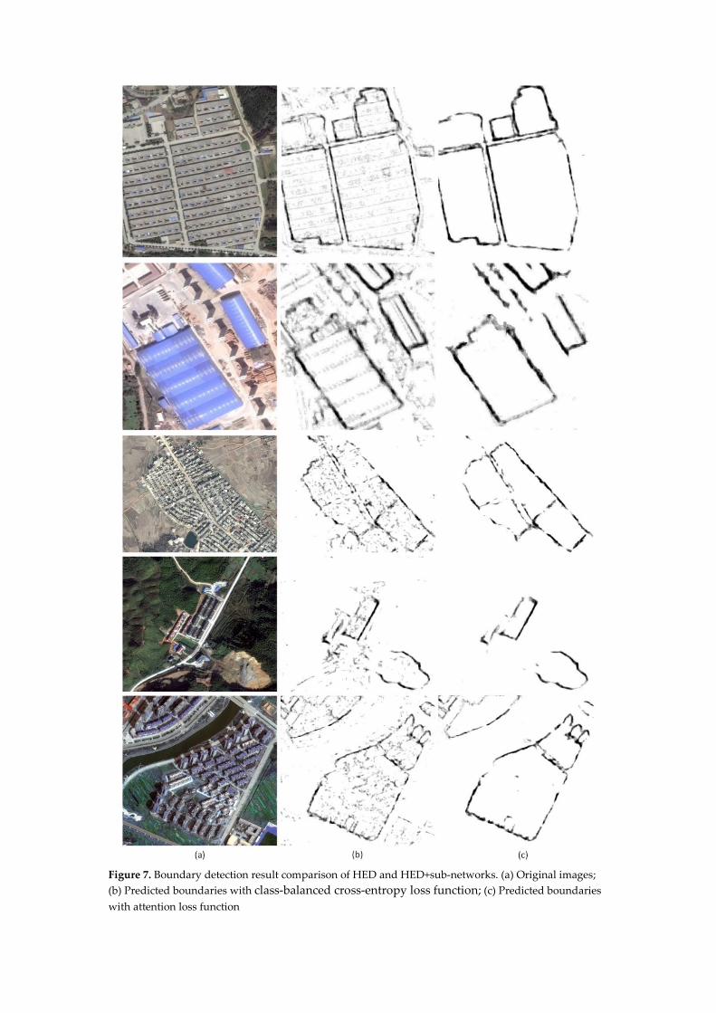
Figure 7. Boundary detection result comparison of HED and HED+sub-networks. (a) Original images;
(b) Predicted boundaries with class-balanced cross-entropy loss function; (c) Predicted boundaries
with attention loss function

Figure 7 shows boundary detection result comparison of HED and HED+ sub-networks.
Although the ���� loss function employed by the HED sub-network can detect common
boundary pixels of the ground objects, the edge pixels inside the ground objects are also
detected. It is hard for ���� loss function to discriminate true positive and false positive edges
where most edge pixels do not belong to boundary. Therefore, as an important part of input
data to the subsequent pixel-wise classification network, the boundary detection results mixed
with false positive edges is not conducive. As the boundary detection results shown in Figure
7, the ��� loss function employed by the HED+ sub-network puts more focus on hard,
misclassified samples and classify the boundary more precise than ���� .
6. Conclusions
DCNNs-based model has been proved to be efficient in the semantic segmentation of
ground objects of construction activities. To support the monitoring of temporary works and
ESAs of railway construction projects, we introduced a novel DCNNs-based monitoring
framework using VHR satellite images. The framework was developed and tested with
Ruichang-Jiujing railway construction project in China. Focusing on classification problems for
target ground objects, the proposed DV3+HED+ network labels the class of each pixel in the
input images. With reference to the previous state-of-the-art semantic segmentation results, the
framework detected and calculate the precise changes among multitemporal images.
The main purpose of this paper is to propose a DCNNs-based classification workflow for
providing reference data to the environmental soil and water conservation supervision
department to reduce the manual labor. The proposed framework has been developed into a
system, which allowed the pixel-wise classification module working as a plugin. We also open
the source code of the DV3+HED+ network on GitHub for researchers who are interesting with
our works (https://github.com/xjock/deeplebv3plus-hedplus). In further studies, multiple
source satellite images need to be considered in order to make the semantic segmentation
monitoring framework more practical.
Acknowledgments: The work is supported by the National Key Research and Development Project under
Grant No. 2018YFE010010001-3.
Author Contributions: Rui Guo designed and performed experiments, analyzed data and wrote the
paper; Na Li supervised the research, and additionally provided comments and revised the manuscript.
Ronghua Liu provided the VHR satellite images and ground truth data. Wei Liu was helpful in improving
the English writing.
Conflicts of Interest: The authors declare no conflicts of interest
References
1. Mountrakis, G.; Im, J.; Ogole, C. Support vector machines in remote sensing: A review. ISPRS J.
Photogramm. Remote Sens. 2011, 66, 247–259.
2. Miller, D.M.; Kaminsky, E.J.; Rana, S. Neural network classification of remote-sensing data.
Comput. Geosci.1995, 21, 377–386.
3. Pal, M. Random forest classifier for remote sensing classification. Int. J. Remote Sens. 2005, 26,
217–222.
4. Blaschke, T. Object-based image analysis for remote sensing. Object-based image analysis for
remote sensing. 2010, 65 (1), 2-16.
5. Lowe, D.G. Object Recognition from Local greScale-Invariant Features. Proc. Int. Conf. Comput.
Vis. 1999, 2, 1150–1157.
6. Dalal, N.; Triggs, B. Histograms of Oriented Gradients for Human Detection. IEEE Comput. Soc.
Conf. Comput. Vis. Pattern Recognit. 2005, 1, 886–893.
7. Chen, L. C., Zhu, Y., Papandreou, G., Schroff, F., Adam, H. Encoder-decoder with atrous
separable convolution for semantic image segmentation. 2018, arXiv:1802.02611v3.

8. Xie S, Tu Z. Holistically-Nested Edge Detection[J]. International Journal of Computer Vision,
2015, 125(1-3):3-18.
9. Wickramasinghe, D. C., Vu, T.T., Maul, T. Satellite remote-sensing monitoring of a railway
construction project. International Journal of Remote Sensing, 2017, 39(6), 1754–1769.
10. Giannico, C., Ferretti, A., Alberti, S. Application of satellite radar interferometry for tunnel and
underground infrastructures damage assessment and monitoring. In Life-Cycle and
Sustainability of Civil Infrastructure Systems: Proceedings of the Third International
Symposium on Life-Cycle Civil Engineering (IALCCE'12), Vienna, Austria, October 3-6, 2012 (p.
420). CRC Press.
11. Lin, J., Wang, Z., Wang, Y., Lin, Y., Du, X. Monitoring abandoned dreg fields of high-speed
railway construction with UAV remote sensing technology. In: International Conference on
Intelligent Earth Observing and Applications 2015. International Society for Optics and
Photonics.
12. Chang, L., Dollevoet, R. P. B. J., Hanssen, R. F. Nationwide railway monitoring using satellite
SAR interferometry. IEEE Journal of Selected Topics in Applied Earth Observations and Remote
Sensing, 2016, 1-9.
13. Arastounia, M. Automated recognition of railroad infrastructure in rural areas from lidar data.
Remote Sensing, 2015, 7(11), 14916-14938.
14. Long, J.; Shelhamer, E.; Darrell, T. Fully convolutional networks for semantic segmentation. In
Proceedings of the 2015 IEEE Conference on Computer Vision and Pattern Recognition (CVPR),
Boston, MA, USA, 7–12 June 2015.
15. Everingham, M.; Eslami, S.A.; Van Gool, L.; Williams, C.K.; Winn, J.; Zisserman, A. The pascal
visual object classes challenge: A retrospective. Int. J. Comput. Vis. 2015, 111, 98–136.
16. Lin, T.-Y.; Maire, M.; Belongie, S.; Hays, J.; Perona, P.; Ramanan, D.; Dollar, P.; Zitnick, C.L.
Microsoft coco: Common objects in context. In Proceedings of the European Conference on
Computer Vision ECCV, Zurich, Switzerland, 6–12 September 2014; pp. 740–755.
17. Vijay, B.; Kendall, A.; Cipolla, R. SegNet: A Deep Convolutional Encoder-Decoder Architecture
for Image Segmentation. arXiv 2015, arXiv:1511.00561.
18. Ronneberger, O.; Fischer, P.; Brox, T. U-Net: Convolutional Networks for Biomedical Image
Segmentation. In Proceedings of the International Conference on Medical image computing and
computer-assisted intervention, Munich, Germany, 5–9 October 2015; pp. 234–241.
19. Lin, G.; Milan, A.; Shen, C.; Reid, I. RefineNet: Multi-Path Refinement Networks for High-
Resolution Semantic Segmentation. arXiv 2016, arXiv:1611.06612.
20. He K., Zhang X., Ren S., et al. Deep Residual Learning for Image Recognition[J]. CVPR, 2016.
21. Chaurasia, A., & Culurciello, E. Linknet: exploiting encoder representations for efficient
semantic segmentation. arXiv 2017, arXiv: 1707.03718.
22. Zhao, H.; Shi, J.; Qi, X.; Wang, X.; Jia, J. Pyramid Scene Parsing Network. arXiv 2016,
arXiv:1612.01105.
23. Yu C., Wang J., Peng C., et al. BiSeNet: Bilateral Segmentation Network for Real-Time Semantic
Segmentation. ECCV 2018.
24. Chen, L.-C.; Papandreou, G.; Kokkinos, I.; Murphy, K.; Yuille, A.L. Semantic Image
Segmentation with Deep Convolutional Nets and Fully Connected CRFs. arXiv 2014,
arXiv:1412.7062v1.
25. Chen, L.-C.; Papandreou, G.; Kokkinos, I.; Murphy, K.; Yuille, A.L. DeepLab: Semantic Image
Segmentation with Deep Convolutional Nets, Atrous Convolution, and Fully Connected CRFs.
arXiv 2016, arXiv:1606.00915v1.
26. Chen, L. C., Papandreou, G., Schroff, F., Adam, H. Rethinking atrous convolution for semantic
image segmentation. arXiv 2017, arXiv: 1706.05587.
27. Penatti, O.A.B.; Nogueira, K.; dos Santos, J.A. Do Deep Features Generalize from Everyday
Objects to Remote Sensing and Aerial Scenes Domains? CVPR 2015.
28. Volpi, M.; Tuia, D. Dense semantic labeling of sub-decimeter resolution images with
convolutional neural networks. IEEE Trans. Geosci. Remote Sen. 2017, 55, 881–893.

29. Liu, Y.; Nguyen, D.; Deligiannis, N.; Ding, W.; Munteanu, A. Hourglass-ShapeNetwork Based
Semantic Segmentation for High Resolution Aerial Imagery. Remote Sens. 2017, 9, 522.
30. Maggiori, E.; Tarabalka, Y.; Charpiat, G.; Alliez, P. High-resolution semantic labeling with
convolutional neural networks. arXiv 2016, arXiv:1611.01962.
31. Liu, P.; Liu, X.; Liu, M.; Shi, Q.; Yang, J.; Xu, X.; Zhang, Y. Building Footprint Extraction from
High-Resolution Images via Spatial Residual Inception Convolutional Neural Network. Remote
Sens. 2019, 11, 830.
32. Marmanis, D.; Schindler, K.; Wegner, J.D.; Galliani, S.; Datcu, M.; Stilla, U. Classification with
an edge: Improving semantic image segmentation with boundary detection. ISPRS Journal of
Photogrammetry and Remote Sensing, 135, 2018, 158-172.
33. Guo, R.; Liu, J.; Li, N.; Liu, S.; Chen, F.; Cheng, B.; Duan, J.; Li, X.; Ma, C. Pixel-Wise
Classification Method for High Resolution Remote Sensing Imagery Using Deep Neural
Networks. ISPRS Int. J. Geo-Inf. 2018, 7, 110.
34. Tian, C., Li, C., Shi, J. Dense Fusion Classmate Network for Land Cover Classification. CVPR
2018.
35. Li, Y., Xu, L., Rao, J., Guo, L., Yan, Z., & Jin, S. A Y-Net deep learning method for road
segmentation using high-resolution visible remote sensing images. Remote sensing letters, 2019,
10(4), 381-390.
36. Wang G, Liang X, Li F. DOOBNet: Deep Object Occlusion Boundary Detection from an Image.
ACCV, 2018.
37. Simonyan, K.; Zisserman, A. Very Deep Convolutional Networks for Large-Scale Image
Recognition. In Proceedings of the 3rd International Conference on Learning Representations,
San Diego, CA, USA, 7–9 May 2015.


