
Dynamic Portfolio Selection
by Augmenting the Asset Space ∗
Michael W. Brandt Pedro Santa-Clara
The Wharton School The Anderson SchoolUniversity of Pennsylvania UCLA
and NBER
First Draft: November 2001
This Draft: December 2002
Abstract
We present a novel approach to dynamic portfolio selection that is nomore difficult to implement than the static Markowitz approach. The ideais to expand the asset space to include simple (mechanically) managedportfolios and compute the optimal static portfolio in this extended assetspace. The intuition is that a static choice among managed portfoliosis equivalent to a dynamic strategy. We consider managed portfolios oftwo types: “conditional” and “timing” portfolios. Conditional portfoliosare constructed along the lines of Hansen and Richard (1987). For eachvariable that affects the distribution of returns and for each basis asset, weinclude a portfolio that invests in the basis asset an amount proportional tothe level of the conditioning variable. Timing portfolios invest in each assetfor a single period, and therefore mimic strategies that buy and sell theasset. We apply our method to a problem of dynamic asset allocation acrossthree assets, using the predictive ability of four conditioning variables.
∗We thank Michael Brennan, John Campbell, Francis Longstaff, Eduardo Schwartz, Rob Stambaugh,Rossen Valkanov, Luis Viceira, and Shu Yan, as well as seminar participants at Barclays Global Investorsand Morgan Stanley Investment Management for helpful comments.

1 Introduction
Several studies have pointed out the importance of dynamic trading strategies to exploit
the predictability of the first and second moments of asset returns and to hedge changes
in the investment opportunities.1 Unfortunately, computing optimal dynamic investment
strategies has proven to be a rather formidable problem. Because closed-form solutions
are only available for a few cases, researchers have explored a variety of numeric methods,
including solving partial differential equations, discretizing the state-space, and using
Monte Carlo simulation. Unfortunately, these techniques are out of reach for most
practitioners and have therefore remained largely in the ivory tower. The workhorse of
portfolio optimization in industry remains the static Markowitz approach.
Our paper presents a novel approach to dynamic portfolio selection that is no more
difficult to implement than the static Markowitz approach. The idea is to expand
the asset space to include simple (mechanically) managed portfolios and compute the
optimal static portfolio within this extended asset space. The intuition is that a static
choice of managed portfolios is equivalent to a dynamic strategy. Put differently,
the optimal dynamic strategy is a fixed combination of a number of naive dynamic
strategies. We consider managed portfolios of two types: “conditional” and “timing”
portfolios. Conditional managed portfolios are constructed along the lines of Hansen and
Richard (1987).2 For each variable that affects the distribution of returns and for each
basis asset we consider a portfolio that invests in the basis asset an amount proportional
to the level of the conditioning variable. Timing portfolios invest in each asset for a
single period. They mimic strategies that buy and sell the asset. Holding a constant
amount of all the timing portfolios related to a single asset approximates a strategy that
holds a constant proportion of wealth in the asset. In contrast, hedging demands will
induce the investor to hold different amounts of the timing portfolios
Our approach is similar in spirit to that of Cox and Huang (1989) and its empirical
implementation by Aıt-Sahalia and Brandt (2002). They solve the dynamic portfolio
problem in two steps. The investor first chooses the optimal portfolio of Arrow-Debreu
securities and then figures out how to replicate this portfolio by dynamically trading the
1See Brandt (2002) for a survey and the references therein.2Hansen and Richard (1987) introduced this idea to develop tests of conditional asset pricing models.
Bansal and Harvey (1996) use conditional portfolios in performance evaluation.
1

basis assets or derivatives on the basis assets. In contrast, we solve the portfolio problem
in one step as the optimal choice across simple dynamic trading strategies. Note also
that the Cox-Huang approach requires financial markets to be complete, for only then
all Arrow-Debreu securities can be replicated, whereas we do not need to assume market
completeness since the investor only chooses among the payoffs of feasible strategies.
In general, our approach relies on sample moments of the long-horizon returns on
the expanded set of assets, consisting of the base assets and the mechanically managed
portfolios. However, if the log returns on the base assets and the log state variables follow
a vector auto-regression (VAR) with normally distributed innovations, as in the line of
research initiated by Campbell and Viceira (1999), these long-horizon moments can all
be expressed in terms of the parameters of the VAR.3 In this special but popular case, we
obtain approximate closed-form solutions for the finite-horizon dynamic portfolio choice
which complement the approximate closed-form solutions for the infinite-horizon case
with intermediate consumption derived by Campbell and Viceira.
The advantage of framing the dynamic portfolio choice problem in a static context
is that all of the statistical tools developed for the Markowitz approach over the years
are at our disposal. Given the popularity of the static Markowitz approach, there is an
extensive literature on its statistical properties and potential refinements. The latter
includes the use of portfolio constraints, shrinkage estimation, and the combination of
the investor’s prior with the information contained in the history of returns.
The paper proceeds as follows. We first describe our approach in section 2.1 and 2.2.
We then illustrate the mechanics of our approach through a simple example in Section
2.3. Section 3 deals with the special case in which the log returns and log state variables
follow a Gaussian VAR and Section 4 discusses briefly how the refinements of the static
Markowitz approach can be directly applied to our approach. We further illustrate our
approach through an empirical application in Section 5 and conclude in Section 6.
2 The Method
We solve a conditional portfolio choice problem with parameterized portfolio weights
of the form xt = θzt, where zt denotes a vector of state variables and θ is a matrix of
3See also the survey by Campbell and Viceira (2002).
2

coefficients. This conditional portfolio choice problem is mathematically equivalent to
solving an unconditional problem with an augmented asset space that includes naively
managed zero-investment portfolios with excess returns of the form zt times the excess
return of each basis asset. We first establish this idea in the context of a single-period
problem and then extend the approach to the multiperiod case. Finally, we illustrate
both cases in a simple example.
2.1 Single-Period Problem
We want to find the optimal portfolio policy under a quadratic criterium on the excess
returns of the portfolio:
max Et
[rpt+1 −
γ
2(rp
t+1)2]
(1)
where γ is a positive constant and rpt+1 = Rp
t+1−Rft is the excess return on the portfolio
from t to t + 1.4 (Throughout this paper we use capital letters to denote gross returns
and lower-case letters to denote excess returns. We date all variables with a subscript
that corresponds to the time at which the variable is known. For example, returns of
risky assets from time t to time t + 1 are denoted Rt+1. The risk-free rate for the same
period is denoted Rft , since that is known at the beginning of the return period.)
Denote the vector of portfolio weights on the risky assets at time t by xt. The above
optimization problem then becomes:
maxxt
Et
[x>t rt+1 − γ
2x>t rt+1r
>t+1xt
], (2)
where rt+1 = Rt+1 − Rft is the vector of excess returns on the N risky assets. By
formulating the problem in terms of excess returns, we are implicitly assuming that the
4We can obtain this criterium from quadratic utility over wealth u(Wt+1) = Wt+1 − a2 W 2
t+1. Thisimplies that the relative risk aversion coefficient is given by κ = a Wt
1−a Wt. We can rewrite this expression
as a Wt = κ1+κ . Now reconsider the utility function:
u(Wt+1) = Wt+1 − a
2(Wt+1)2 = WtR
pt+1 −
a
2(WtR
pt+1)
2
= Wt
[Rp
t+1 −a
2Wt(R
pt+1)
2]
= Wt
[Rp
t+1 −κ
2(1 + κ)(Rp
t+1)2
],
where Rpt+1 denotes the gross return on the investor’s portfolio. For a given (constant) initial wealth
Wt, maximizing the expectation of the function above is equivalent to the problem (1), with γ = κ1+κ .
3

remainder of the value of the portfolio is invested in the risk-free asset with return Rft .
When the returns are iid and the portfolio weights are constant through time, xt = x,
we can replace the conditional expectation with an unconditional one and solve for:
x =1
γE
[rt+1r
>t+1
]−1E [rt+1] . (3)
This is the well-known Markowitz solution, which can be implemented in practice by
replacing the population moments by sample averages:
x =1
γ
[ T−1∑t=1
rt+1r>t+1
]−1[ T−1∑t=1
rt+1
]. (4)
(Notice that the 1/T terms in the sample averages cancel.)
Consider now the more realistic case of non-iid returns and assume that the optimal
portfolio policies are linear in a vector of K state variables (the first of which we will
take to be a constant):
xt = θzt, (5)
where θ is an N ×K matrix. Our problem is then:
maxθ
Et
[(θzt)
>rt+1 − γ
2(θzt)
>rt+1r>t+1(θzt)
]. (6)
We can use the following result from linear algebra:
(θzt)>rt+1 = z>t θ>rt+1 = vec(θ)>(zt ⊗ rt+1), (7)
where vec(·) is the operator that piles up the columns of a matrix into a vector and ⊗is the Kronecker product of two matrices, and write:
x = vec(θ) (8)
rt+1 = zt ⊗ rt+1 (9)
Our problem can now be written as:
maxx
Et
[x>rt+1 − γ
2x>t rt+1r
>t+1xt
]. (10)
4

Since the same x maximizes the conditional expected utility at all dates t, it also
maximizes the unconditional expected utility:
maxx
E[x>rt+1 − γ
2x>t rt+1r
>t+1xt
], (11)
which corresponds simply to the problem of finding the unconditional portfolio weights
x for the expanded set of (N × K) assets with returns rt+1. The expanded set of
assets can be interpreted as managed portfolios, each of which invests in a single basis
asset an amount proportional to the value of one of the state variables. We term these
“conditional portfolios.”
It follows that the optimal x is:
x =1
γE
[rt+1r
>t+1
]−1E [rt+1]
=1
γE
[(ztz
>t )⊗ (rt+1r
>t+1)
]−1E [zt ⊗ rt+1] ,
(12)
which we can again implement by replacing the population moments by sample averages:
x =1
γ
[ T∑t=0
(ztz>t )⊗ (rt+1r
>t+1)
]−1[ T∑t=0
zt ⊗ rt+1
]. (13)
From this solution we can trivially recover the weight invested in each of the basis assets
by adding the corresponding products of elements of x and zt.
Note that the solution (13) depends only on the data and hence does not require any
assumptions besides stationarity about the distribution of returns, including assumptions
about how the return moments depend on the state variables. The state variables
can predict time-variation in first, second, and, if we consider more general utility
functions, even higher-order moments of returns. As Brandt (1999) and Aıt-Sahalia and
Brandt (2001) emphasize, the advantage of focusing directly on the portfolio weights is
that we bypass the estimation of the conditional return distribution. This intermediate
estimation step typically involves ad-hoc distributional assumptions and inevitably
misspecified models for the conditional moments of returns. Estimating the conditional
portfolio weights in a single step is robust to misspecification of the conditional return
distribution. It also results in more precise estimates if the dependence of the optimal
5

portfolio weights on the state variables is less noisy than the dependence of the return
moments on the state variables.
Furthermore, the assumption that the portfolio weights are linear functions of the
state variables is innocuous because zt can include non-linear transformations of a set
of more basic state variables yt. This means that the linear portfolio weights can be
interpreted as a more general portfolio policy function xt = g(yt) for any g(·) that
can be spanned by a polynomial expansion in the more basic state variables yt. In
other words, our approach can in principle accommodate very general dependence of the
optimal portfolio weights on the state variables.
Since we express the portfolio choice problem in an estimation context, we can
use standard sampling theory to get standard errors for the portfolio weights and test
hypotheses about them. Specifically, following Britten-Jones (1999), we can interpret
the solution (13) as being proportional (with constant of proportionality 1/γ) to the
coefficients of a standard least-squares regression of a vector of ones on the returns rt+1.
As a result, we can compute standard errors for the coefficients x as the standard errors
of the regression coefficients, which can be used to test whether some state variable is a
significant determinant of the portfolio policy. Using our notation, the covariance matrix
of the vector x is:1
γ2
1
T −N ×K(ιT − rx)>(ι− rx)(r>r)−1 (14)
where ιT denotes a T × 1 vector of ones and r is a T ×K matrix with the time series of
returns of the K managed portfolios.
Finally, notice that we can easily extend our approach to allow some or all of the
state variables to be asset-specific (e.g., firm size or price ratios). Simply include in
the static problem the conditional portfolios constructed with the asset-specific state
variables multiplied by their respective asset.
2.2 Multiperiod Problem
The idea of augmenting the asset space with naively managed portfolios extends to the
multiperiod case. Consider an investor who maximizes the following two-period mean-
variance objective:
max Et
[rpt→t+2 −
γ
2(rp
t→t+2)2], (15)
6

where rp,t→t+2 denotes the excess return of a two-period investment strategy:
rp,t→t+2 =(Rf
t + x>t rt+1
)(Rf
t+1 + x>t+1rt+2
)−Rft R
ft+1
= x>t (Rft+1rt+1) + x>t+1(R
ft rt+2) + (x>t rt+1)(x
>t+1rt+2).
(16)
The first line of this expression shows why we call rp,t→t+2 a two-period excess return.
The investor borrows a dollar at date t and allocates it to the risky and riskfree assets
according to the first-period portfolio weights xt. After the first period, at date t + 1,
the one-dollar investment has resulted in (Rft + x>t rt+1) dollars, which the investor then
allocates again to the risky and riskfree assets according to the second-period portfolios
weights xt+1. Finally, at date t + 2, the investor has (Rft + x>t rt+1)(R
ft+1 + x>t+1rt+2)
dollars but must repay the bank Rft R
ft+1 dollars for the principal and interest of the
one-dollar loan. The remainder is the two-period excess return.
The second line of equation (16) decomposes this two-period excess return into three
terms. The first two terms have a natural interpretation as the excess return of investing
in the riskfree rate in the first (second) period and in the risky asset in the second (first)
period.5 Notice that the portfolio weights on these two intertemporal portfolios are the
same as the weight on the risky asset in the first and second period, respectively. The
third term in this expression captures the effect of compounding.
Comparing the first two terms to the third, notice that the latter is two orders of
magnitude smaller than the former. The return (x>t rt+1)(x>t+1rt+2) is a product of two
single-period excess returns, which means that its units are 1/100th of a percent. The
returns on the first two portfolios, in contrast, are products of a gross return (Rft or
Rft+1) and an excess return (rt+1 or rt+2), so their units are percent.
Given that the compounding term is orders of magnitude smaller than the two
intertemporal portfolios, we will for now ignore it. This approximation is exact for
an investor with exponential utility, and introduces a small approximation error in the
quadratic utility case we are studying. (See Section 4.3 for a recursive solution that
eliminates the approximation error.) In that case, the two-period portfolio choice is
5To see that x>t (Rft+1rt+1) is a two-period excess return from investing in risky assets in the first
period and the riskfree asset in the second period, just follow the argument above with xt+1 = 0.Investing the first-period proceeds of (Rf
t + x>t rt+1) in the riskfree asset in the second period yields(Rf
t +x>t rt+1)Rft+1. After paying back Rf
t Rft+1, the investor is left with an excess return of x>t (Rf
t rt+1).
7

simply a choice between two intertemporal portfolios, one that holds the risky asset in
the first period only and the other that holds the risky asset in the second period only.
We term these “timing portfolios.” We can solve the dynamic problem as a simple static
choice between these two managed portfolios. In particular, for the two-period case, the
sample analogue of the optimal portfolio weights are given by:
x =1
γ
[ T−2∑t=1
rt→t+2r>t→t+2
]−1[ T−2∑t=1
rt→t+2
], (17)
where rt→t+2 = [Rft+1rt+1, R
ft rt+2]. The first set of elements of x (the ones corresponding
to the returns Rft+1rt+1) then represents the fraction of wealth invested in the risky assets
in the first period and the second set of elements (corresponding to Rft rt+2) are for the
risky assets in the second period.
In a general H-period problem, we proceed in exactly the same fashion. We construct
a set of timing portfolios:
rt→t+H =
H−1∏
i=0i6=j
Rft+irt+j+1
H−1
j=0
(18)
where each term represents a portfolio that invests in risky assets in period t + j and
in the riskfree rate in all other periods t + i with i 6= j. The sample analogue of the
optimal portfolio weights are then again given by the static solution:
x =1
γ
[ T−H∑t=1
rt→t+H r>t→t+H
]−1[ T−H∑t=1
rt→t+H
]. (19)
Notice, however, that as the length of the horizon H increases we loose observations
for computing the mean and covariance matrix of rt→t+H , which introduces a trade-off
between the length of the horizon and the statistical precision of the solution. It is
also important to realize that, in contrast to a long-horizon buy-and-hold problem, the
random components of the timing portfolios are non-overlapping. We thereby avoid the
usual statistical problems associated with overlapping long-horizon returns.
We can naturally combine the ideas of conditional portfolios and timing portfolios.
8
For this, we replace the risky returns rt+j+1 in equation (18) with the conditional portfolio
returns zt+j ⊗ rt+j+1. The resulting optimal portfolio weights x from equation (19) then
provide the optimal allocations to the conditional portfolios at each time t + j.
The obvious appeal of our approach is its simplicity. Naturally, this simplicity comes
with several drawbacks. First, the way we solve the dynamic problem can be too data-
intensive for problems with very long horizons. For example, suppose we want to solve a
ten-year portfolio choice problem with quarterly rebalancing based on a 60-year post-war
sample of quarterly returns and state variable realizations. Since each timing-portfolio
involves a ten-year return, we would only have six independent observations to compute
the moments of the timing-portfolio returns and hence the optimal portfolio weights. The
obvious way to overcome this data issue is to impose a statistical model for the returns
and state variables which allows us to compute the long-horizon moments analytically
(or by simulations) from the parameters of the statistical model. Specifically, if the
log returns on the base assets and the log state variables follow a VAR with normally
distributed innovations, the long-horizon moments can be expressed in terms of the
parameters of the VAR. This use of a statistical model allows us to solve dynamic
portfolio choice problems with arbitrarily long horizons using finite data samples. We
elaborate on this idea in Section 3.
Another drawback of our approach is that by circumventing the use of dynamic
programming we cannot solve portfolio choice problems with endogenous state variables
which depend in some form or another on the decisions the investor made in previous
periods. This includes problems in which the optimal portfolio weights depend on the
investor’s wealth, as in the case of preferences with non-constant relative risk aversion, or
on the investor’s previous portfolio holdings, as in the case of transaction costs. If some
of the state variables are endogenous, we have to combine our approach with traditional
recursive dynamic programming techniques such as discretizing the state space.
9

2.3 A Simple Example
To illustrate more concretely the mechanics of our approach, consider a time series of
only six observations (for simplicity) of two risky assets, stocks s and bonds b:
rs1 rb
1
rs2 rb
2
· · · · · ·rs6 rb
6
(20)
The optimal static portfolio in equation (4) directly gives us the weight xs invested in
the stock and the weight xb invested in the bond (with the remainder invested in the
risk-free asset). The solution takes into account the sample covariance matrix of asset
returns and the vector of sample mean excess returns.
Suppose that there is one conditioning variable, such as the dividend yield or the
spread between long and short Treasury yields, which affects the conditional distribution
of returns. We observe a time series of this state variable:
z0
z1
· · ·z5
, (21)
where the dating reflects the fact that z is known at the beginning of each return period.
We can take into account the information in the conditioning variable by estimating a
portfolio policy which depends on the value of the state variable. For this, we expand
the matrix of returns (20) in the following manner:
rs1 rb
1 z0rs1 z0r
b1
rs2 rb
2 z1rs2 z1r
b2
· · · · · · · · · · · ·rs6 rb
6 z5rs6 z5r
b6
(22)
and compute the optimal static portfolio of this expanded set of assets. This static
solution gives us a vector of four portfolio weights x. We can find the weight invested in
10

stocks at each time by using the first and third elements of x, xst = x1 + x3zt. Similarly,
the weight invested in the bond at each time is xbt = x2 + x4zt. Note that when we
use the Markowitz solution (4) on the matrix of returns of the expanded asset set (22),
the covariance matrix and vector of means takes into account the covariances among
returns and between returns and lagged state variables. The latter covariances capture
the impact of predictability of returns on the optimal portfolio policy.
Consider now a two-period portfolio choice problem. We construct the matrix of
returns to the timing portfolios as described in equation (18):
rs1R
f1 Rf
0rs2 rb
1Rf1 Rf
0rb2
rs3R
f3 Rf
2rs4 rb
3Rf3 Rf
2rb4
rs5R
f5 Rf
4rs6 rb
5Rf5 Rf
4rb6
(23)
This matrix contains two-period non-overlapping returns of four trading strategies. The
corresponding optimal portfolio vector x gives us the weights on “stocks in period 1,”
“stocks in period 2,” “bonds in period 1,” and “bonds in period 2.” The covariance
matrix and vector of means which show up in the static portfolio solution account for
the contemporaneous covariances of returns as well as the one-period serial-covariances
of returns. The latter covariances induce hedging demands.
Finally, we can consider a two-period problem with the conditioning variable. The
returns of the expanded asset set are:
rs1R
f1 Rf
0rs2 rb
1Rf1 Rf
0rb2 z0r
s1R
f1 Rf
0z1rs2 z0r
b1R
f1 Rf
0z1rb2
rs3R
f3 Rf
2rs4 rb
3Rf3 Rf
2rb4 z2r
s3R
f3 Rf
2z3rs4 z2r
b3R
f3 Rf
2z3rb4
rs5R
f5 Rf
4rs6 rb
5Rf5 Rf
4rb6 z4r
s5R
f5 Rf
4z5rs6 z4r
b5R
f5 Rf
4z5rb6
. (24)
The optimal portfolio of these eight assets now includes the weight on “stocks in period
1, conditional on the level of z,” for example. The portfolio solution takes into account
the covariances between returns and state variables over subsequent periods.
11
3 Optimal Portfolio Weights Implied by a VAR
As we mentioned above, our approach is too data-intensive for solving portfolio choice
problems with very long horizons. However, this issue can be overcome by imposing a
statistical model for the returns and state variables. For example, consider a problem
with a single risk asset and one conditioning variable and assume that the log (gross)
return and log conditioning variable evolve jointly according to the following restricted
VAR with normally distributed innovations:
[ln Rt+1
ln zt+1
]=
[a1
a2
]+
[b1
b2
]ln zt + εt+1, (25)
where εt+1 ∼ N[0, Ω]. For notational convenience, consider the following expanded VAR:
ln Yt+1 = A + B ln Yt + νt+1, (26)
where ln Yt+1 = [ln Rt+1, ln zt+1, ln zt + ln Rt+1]> and ηt+1 ∼ N[0, Γ] with
A =
a1
a2
a1
, B =
0 b1 0
0 b2 0
0 b1 + 1 0
, and Γ =
ω11 ω12 ω11
ω12 ω22 ω12
ω11 ω12 ω11
, (27)
where ωij are the elements of the covariance matrix Ω. The first two unconditional
moments of this expanded VAR are given by:
µ ≡E[ln Yt+1] = (I −B)−1A
vec(Σ) ≡ vec(Var[ln Yt+1]) = (I −B ⊗B)vec(Γ).(28)
3.1 Single-Period Problem
Consider first the single-period portfolio choice. Following equation (9), we construct
excess returns on the managed portfolios:
rt+1 = [Rt+1 −Rf , zt(Rt+1 −Rf )]>
= ΛYt+1 + λ,(29)
12

where
Λ =
[1 0 0
0 −Rf 1
]and λ =
[−Rf
0
]. (30)
The optimal single-period portfolio choice for the expanded asset space, provided in
equation (13), depends on the first two moments of these returns, which are given by:
E[rt+1] = ΛE[Yt+1] + λ and Var[rt+1] = ΛVar[Yt+1]Λ>, (31)
where from the joint log-normality of Yt+1 and the unconditional moments of the VAR:
E[Yt+1] = exp
E[ln Yt+1] +
1
2Diag [Var[ln Yt+1]]
Var[Yt+1] =(
expVar[ln Yt+1]
− 1)E[Yt+1]E[Yt+1]
>.
(32)
The moments in equation (31), and hence the optimal portfolio weights, can therefore
be evaluated using the unconditional moments of the VAR in equation (28).
3.2 Multiperiod Portfolio Choice
Consider next a two-period dynamic problem. The excess returns on the conditional
and timing portfolios are:
rt→t+2 = [(Rt+1 −Rf )Rf , zt(Rt+1 −Rf )Rf
︸ ︷︷ ︸stocks in period 1,conditional on z
, Rf (Rt+2 −Rf ), Rfzt+1(Rt+2 −Rf )︸ ︷︷ ︸stocks in period 2,conditional on z
]
= Rf
( [Λ 0
0 Λ
][Yt+1
Yt+2
]+
[λ
λ
]> ).
(33)
The corresponding first and second moments are:
E[rt→t+2] = Rf
( [Λ 0
0 Λ
]E
[Yt+1
Yt+2
]+
[λ
λ
] )
Var[rt→t+2] = (Rf )2
[Λ 0
0 Λ
]Var
[Yt+1
Yt+2
][Λ> 0
0 Λ>
],
(34)
13

where:
E
[Yt+1
Yt+2
]= exp
E
[ln Yt+1
ln Yt+2
]+
1
2Diag
[Var
[ln Yt+1
ln Yt+2
]]
Var
[Yt+1
Yt+2
]=
(exp
Var
[ln Yt+1
ln Yt+2
]− 1
)E
[Yt+1
Yt+2
]E
[Yt+1
Yt+2
]> (35)
and from the unconditional moments of the VAR:
E
[ln Yt+1
ln Yt+2
]=
[µ
µ
]
Var
[ln Yt+1
ln Yt+2
]=
[Σ BΣ
BΣ Σ
].
(36)
Finally, consider an N -period dynamic problem. Using basic matrix algebra, the
excess returns on the conditional and timing portfolios can be written as:
rt→t+N =(Rf
)N−1((
IN ⊗ Λ)
Yt+1
· · ·Yt+N
+
(ιN ⊗ λ
)), (37)
where IN and ιN respectively denote an N -dimensional identity matrix and vector of
ones. The corresponding first and second moments are:
E[rt→t+N ] =(Rf
)N−1((
IN ⊗ Λ)E
Yt+1
· · ·Yt+N
+
(ιN ⊗ λ
))
Var[rt→t+N ] =(Rf
)2(N−1)(IN ⊗ Λ
)Var
Yt+1
· · ·Yt+N
(IN ⊗ Λ>
),
(38)
14
where:
E
Yt+1
· · ·Yt+N
= exp
E
ln Yt+1
· · ·ln Yt+Nfs
+
1
2Diag
Var
ln Yt+1
· · ·ln Yt+N
Var
Yt+1
· · ·Yt+N
=
exp
Var
ln Yt+1
· · ·ln Yt+N
− 1
E
Yt+1
· · ·Yt+N
E
Yt+1
· · ·Yt+N
> (39)
and:
E
Yt+1
· · ·Yt+N
= ιN ⊗ µ
Var
Yt+1
· · ·Yt+N
=
B0 B1 B2 · · · BN−1
B1 B0 B1 · · · BN−2
· · · · · · · · · · · · · · ·BN−1 BN−2 BN−3 · · · B0
⊗ Σ.
(40)
To summarize, the optimal portfolio weights for the N -period dynamic problem with
conditional and timing portfolios, which depend on the first and second moments of the
managed portfolio returns, can be evaluated analytically using the coefficient matrix B
and the unconditional moments µ and Σ of the VAR (which in turn depend on A, B,
and Γ). Since we can estimate the VAR with a relatively modest time-series of returns
and state variable realizations, we can solve dynamic portfolio choice problems with
arbitrarily long horizons using finite data samples in this VAR context.
4 Extensions and Refinements
Our approach can be extended and refined along a number of directions. In this
section, we show how to generalize the investor’s utility function, how to compute robust
portfolio weights even with large numbers of assets, and offer an iterative solution to the
multiperiod portfolio problem which takes compounding of returns into account.
15
4.1 Objective Functions
The estimation approach can be extended to an arbitrary utility function u(Wt+1). In
that case, we solve the problem:
maxθ
1
T
T−1∑t=0
u(Rft + (θzt)
>rt+1) (41)
or the corresponding first-order conditions, using numerical optimization methods.
Using a quadratic objective as we have done in the previous sections can be seen as an
approximation of more general utility functions. For increased precision, Brandt, Goyal,
and Santa-Clara (2001) offer a fourth-order expansion to CRRA utility functions and
show that this expansion is highly accurate for investment horizons of up to one year,
even when returns are far from normally distributed. With this fourth-order expansion,
the optimal portfolio weights have a semi-closed form expression in terms of the moments
of returns up to the fourth order. It is straightforward to use this expansion approach
in our extended asset space approach.
We can also consider benchmarks in the objective function. Frequently, money
managers are evaluated on their performance relative to a benchmark portfolio over a
given period. Such problems can easily be solved with our approach. Simply use returns
of the basis assets in excess of the index (instead of in excess of the riskfree interest rate),
Rt − Ritι, in the portfolio optimization. The objective function defined on these excess
returns thus defines a gain from beating the benchmark with low tracking error. The
optimal portfolio weights can be interpreted as deviations from the benchmark, usually
termed “active” weights.
Finally, we can expand the mean-variance objective to penalize covariance with the
return on a particular portfolio such as the market, rm.6 In this case, the objective
would be:
max1
T
T−1∑t=0
[rpt+1 −
γ
2(rp
t+1)2 − λrp
t+1rmt+1
](42)
6Or, similarly, penalize covariance with consumption growth.
16
The solution in the static case is:
x =1
γ
[ T−1∑t=1
rt+1r>t+1
]−1[ T−1∑t=1
(1− rmt+1)rt+1
]. (43)
which can trivially be extended to the conditional and multiperiod problems.
4.2 Constraints, Shrinkage, and Prior Views
A benefit of framing the dynamic portfolio problem in a static context is that we have at
our disposal all of the refinements of the Markowitz approach developed over the years.
These include the use of portfolio constraints to avoid extreme positions (e.g., Frost
and Savarino, 1988; Jagannathan and Ma, 2000), the use of shrinkage to improve the
estimates of the means (e.g., Jobson and Korkie, 1981) as well as of the covariance matrix
(e.g., Ledoit, 1995), and the combination of the investor’s prior from an alternative
data source or the belief in a pricing model with the information contained in returns
(e.g., Treynor and Black, 1973; Black and Litterman, 1992).
For the last approach, which is particularly appealing, a natural prior is that the
weights on the basis assets adhere to some unconditional pricing model or observed
market weights and that the weights on the conditional portfolios are zero. Suppose
that the estimated portfolio weight on asset i is of the form xit = a + bzt, and assume
that z has been standardized to have mean zero. We would shrink a towards the market
capitalization weight of the asset and b towards zero. The shrinkage weights can be
determined from the standard errors in the estimates of a and b, coupled with a prior
on the efficiency of the market.
4.3 Recursive Solutions
We showed in Section 2.2 how to approximate the solution to a multiperiod portfolio
problem by ignoring the compounding of returns. We can actually solve the dynamic
portfolio policy exactly in a recursive manner. The first step consists of solving the
portfolio problem with one period left before the terminal date. This is a one-period
problem that can be solved along the lines of Section 2.1. Then, we move back one period
and consider the problem faced by the investor with two periods to go. We compound
17

each asset’s one-period return with the return on the optimal portfolio in the subsequent
period. Then, we compute the optimal static portfolio with these compounded returns.
This gives us the returns of the optimal two-period portfolio policy, which can be used
to compute the optimal portfolio for a three-period horizon. We iterate in this manner
to obtain the optimal policy of the desired horizon.
This approach can be easily explained with the simple example of Section 2.3. We
take the time series of returns in the matrix (20), and solve a one-period portfolio
problem based on the returns with even-numbered time indices:
rs2 rb
2
rs4 rb
4
rs6 rb
6
(44)
The solution to this problem gives us an estimate of the returns of the optimal portfolio
policy at each of these dates, rp2, rp
4, and rp6. We can now compound the even-numbered
returns on stocks and bonds with the optimal portfolio return on the subsequent period:
Rs1R
p2 − 1 Rb
1Rp2 − 1
Rs3R
p4 − 1 Rb
3Rp4 − 1
Rs5R
p6 − 1 Rb
5Rp6 − 1
(45)
and compute the optimal portfolio policy for this one-period problem.
5 Application
There is substantial evidence that economic variables related to the business cycle
can forecast stock and bond returns. For instance, Campbell (1991), Campbell and
Shiller (1988), Fama (1990), Fama and French (1988,1989), Hodrick (1992), and Keim
and Stambaugh (1986) report evidence that the stock market can be forecasted by
variables such as the dividend-price ratio, the short-term interest rate, the term spread,
and the credit spread. We use these four conditioning variables in a simple application
of our method to the dynamic portfolio choice between stocks, bonds, and cash. This
application is similar to Brennan, Schwartz, and Lagnado (1997) and Campbell, Chan,
18

and Viceira (2001).7
We take the stock to be the CRSP value-weighted market index, the bond to be the
index of long-term Treasuries constructed by Ibbotson Associates, and cash to be the
three-month Treasury bill, also obtained from Ibbotson Associates. The dividend-price
ratio (D/P) is calculated as the difference between the log of the last twelve month
dividends and the log of the current price index of the CRSP value-weighted index.
The relative Treasury bill (Tbill) stochastically detrends the raw series by taking the
difference between the Treasury bill rate and its twelve-month moving average. The term
spread (Term) is calculated as the difference between the yield on long term government
bonds and the Treasury bill rate, also obtained from Ibbotson Associates. The default
spread (Default) is calculated as the difference between the yield on BAA- and AAA-
rated corporate bonds, obtained from the FRED database. For all these variables, we
have monthly data from January of 1927 to December of 2000. Finally, we standardize
the variables to ease the interpretation of the coefficients of the portfolio policy.
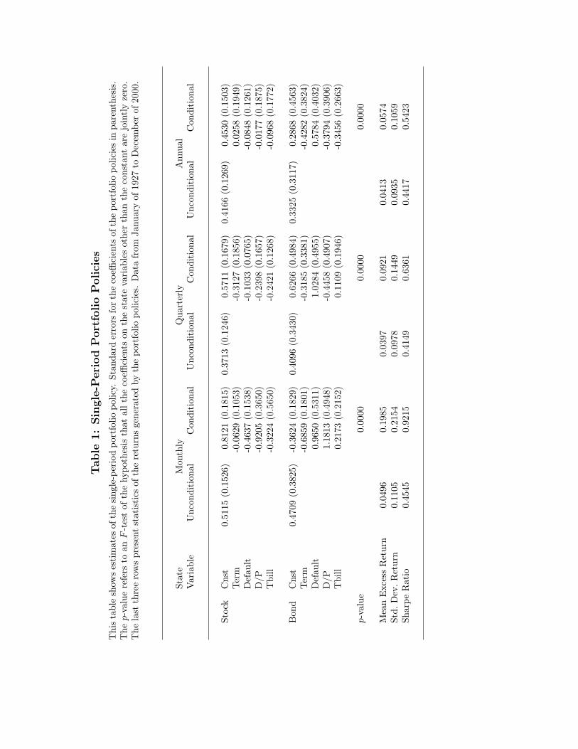
Table 1 reports the results for both unconditional and conditional portfolio policies
at monthly, quarterly, and annual holding periods. We set γ = 4 in all cases, as this
leads to an unconditional asset allocation that holds a small but positive amount in cash,
which is roughly similar to portfolios typically recommended by financial consultants.
There are some differences in the unconditional portfolio weights across the three
holding periods. With monthly rebalancing, the weight on equities is 51.15 percent,
whereas it is only 37.13 and 41.66 percent at the quarterly and annual frequencies,
respectively. This pattern is due to differences in the joint distribution of stock and
bond excess returns over the different holding periods. In particular, there is a small
amount of positive serial correlation at the monthly frequency that turns negative at the
quarterly and annual frequencies. This makes the volatility of stock and bond returns
lower at the monthly frequency.
The conditional policies are quite sensitive to the state variables. For the monthly
conditional policy, the coefficients of the bond weight on Term, Default, and D/P, as
well as the coefficient of the stock weight on Default and D/P are all significant at the 95
7Brennan, Schwartz, and Lagnado (1997) label the dynamic portfolio choice which hedges changes ininvestment opportunities as “strategic asset allocation,” in contrast to the myopic problem of “tacticalasset allocation” which only takes into account the conditional distribution of returns one period ahead.
19

percent level. Furthermore, the average weight held in stocks by the conditional policy
is 81.21 percent, which significantly exceeds the corresponding unconditional weight
of 51.15 percent. The average weight on bonds of the conditional policy is actually
negative, −36.24 percent, compared to the unconditional weight of 47.09 percent. An
F -test of the hypothesis that all coefficients on the state variables are equal to zero
has a p-value of zero. Finally, the (annualized) Sharpe ratio of the conditional policy
is 0.92, which is twice that of the unconditional policy of 0.46. Overall, it is clear that
the conditional return distribution is very different on average than the unconditional
return distribution.
The results are less pronounced for the longer holding periods. At the quarterly
frequency, for example, only the coefficients of the bond weight on Default and of the
stock weight on Tbill are significant. The hypothesis that all coefficients on the state
variables are zero is still rejected with a p-value of zero. More importantly, the Sharpe
ratio of the conditional policy is still 1.5 times that of the unconditional policy, 0.64
versus 0.41. The results for the annual policy are qualitatively similar, with an increase
in Sharpe ratio from 0.44 to 0.54. Judging by the relative increase in the Sharpe ratio,
the conditioning information becomes less important as the holding period decreases.
Figure 1 displays the time series of portfolio weights of the conditional policies. For
comparison, the figure also shows the unconditional portfolio weights. The shorter the
holding period, the more extreme positions the policies take at times. It is striking that
the conditional policies can be substantially different at different frequencies.
As mentioned earlier, by focussing directly on the portfolio weights we capture time-
variation in the entire return distribution as opposed to just the risk premia. To get
a sense for the importance of this aspect of our approach, we compare the conditional
policies to more traditional strategies based on predictive return regressions. Specifically,
we regress the excess stock and bond returns on the state variables and then use one-
period ahead forecasts (in sample) of the conditional means along with an estimate of
the unconditional covariance matrix to form portfolio weights. Table 2 compares the
two approaches, and Figure 2 plots the time series of portfolio weights on stocks.
The advantage of our approach is most striking at the quarterly frequency. Both
strategies generate an average premium of about nine percent per year, but our
conditional strategy has a volatility that is less than half that of the regression-based
20
strategy, 14.5 versus 32.6 percent, resulting in a Sharpe ratio that is more than twice
as large. The investor would be willing to pay an annual fee of more than 16 percent
to obtain this improved performance associated with exploiting the joint time-variation
of the entire return distribution, as opposed to exploiting just the time-variation of the
mean returns. Although the differences between the strategies are less dramatic at the
monthly and annual frequencies, the conclusion nevertheless holds. The fee the investor
is willing to pay for using our conditional strategy is about two percent for monthly
returns and more than four percent for annual returns. It is interesting to note that
as the holding period increases, the benefit of our approach shifts from generating a
substantially higher expected return at a slightly higher level of risk to generating a
slightly lower expected return at a substantially lower level of risk.
Table 3 reports the portfolio weights of the multiperiod portfolio policy for a one-
year horizon with monthly or quarterly rebalancing. For simplicity, we consider only the
unconditional strategy and the conditional strategy with a single state variable, Tbill.
The table reports the estimated portfolio weights for month one, four, eight, and twelve
as well as for all four quarters of the twelve-month or four-quarter problem, respectively.
With monthly rebalancing, the weight on stocks decreases and the weight on bonds
increases as the end of the horizon approaches. This horizon pattern is roughly the same
for the unconditional and conditional policies, which means that it is generated by the
serial-covariance structure of the returns on the basis assets. With quarterly rebalancing,
the unconditional and average conditional (the constant term in the conditional policy)
stock holdings are similar to each other and to the results for monthly rebalancing.
The unconditional and average conditional bond holdings, in contrast, are very different
from each other. In the unconditional policy, the bond holding increases from −4 to
56 percent as the end of the horizon approaches, while in the conditional policy the
average bond holding decreases from −17 to −27 percent. This difference in the horizon
patterns can only be attributed to the serial-covariance structure of the conditional
portfolio returns, which illustrates the importance of augmenting the asset space in this
multiperiod problem.
Finally, notice that the Sharpe ratios of the multiperiod policies are higher than in
the corresponding single-period case. Consistent with the prediction of intertemporal
portfolio theory, both mean and volatility of the portfolio returns are both lower.
21

Given the serial-covariance structure in the data, the investor sacrifices mean return
for intertemporal diversification.
6 Conclusion
We presented a simple closed-form approach for dynamic portfolio selection. The
solution extends the Markowitz approach to the choice between base assets, conditional
portfolios that invest in each asset a weight proportional to some conditioning variable,
and timing portfolios that invest in each asset in a single period. The intuition underlying
our approach is that the static choice of these mechanically managed portfolios is
equivalent to a dynamic strategy. Our hope is that by making dynamic portfolio selection
no more difficult to implement than the static Markowitz approach, it will finally leave
the confines of the ivory tower and make its way into the day-to-day practice of the
investment industry.
22

References
Aıt-Sahalia, Yacine, and Michael W. Brandt, 2001, Variable selection for portfolio choice,
Journal of Finance 56, 1297–1351.
, 2002, Portfolio and consumption choice with option-implied state prices,
Working Paper, Princeton University.
Bansal, Ravi, and Campbell R. Harvey, 1996, Performance evaluation in the presence of
dynamic trading strategies, Working Paper, Duke University.
Black, Fisher, and Robert Litterman, 1992, Global portfolio optimization, Financial
Analysts Journal 48, 28–43.
Brandt, Michael W., Amit Goyal, and Pedro Santa-Clara, 2001, A simulation approach
to dynamic portfolio choice, Working Paper, UCLA.
, 1999, Estimating portfolio and consumption choice: A conditional method of
moments approach, Journal of Finance 54, 1609–1646.
, 2002, The econometrics of portfolio choice problems, in Yacine Aıt-Sahalia, and
Lars P. Hansen, ed.: Handbook of Financial Econometrics.
Brennan, Michael J., Eduardo S. Schwartz, and Ronald Lagnado, 1997, Strategic asset
allocation, Journal of Economic Dynamics and Control 21, 1377–1403.
Britten-Jones, Mark, 1999, The sampling error in estimates of mean-variance efficient
portfolio weights, Journal of Finance 54, 655–671.
Campbell, John Y., Yeung Lewis Chan, and Luis M. Viceira, 2001, A multivariate model
of strategic asset allocation, Working Paper, Harvard University.
Campbell, John Y., and Robert J. Shiller, 1988, Stock prices, earnings, and expected
dividends, Journal of Finance 43, 661–676.
Campbell, John Y., and Luis M. Viceira, 1999, Consumption and portfolio decisions
when expected returns are time varying, Quarterly Journal of Economics 114.
, 2002, Strategic Asset Allocation: Portfolio Choice for Long-Term Investors.
23

, 1991, A variance decomposition for stock returns, Economic Journal 101, 157–
179.
Cox, John C., and Chi-Fu Huang, 1989, Optimal consumption and portfolio policies
when asset prices follow a diffusion process, Journal of Economic Theory 49, 33–83.
Fama, Eugene F., and Kenneth R. French, 1988, Permanent and temporary components
of stock prices, Journal of Political Economy 96, 246–273.
, 1989, Business conditions and expected returns on stocks and bonds, Journal
of Financial Economics 25, 23–49.
, 1990, Stock returns, expected returns, and real activity, Journal of Finance 45,
1089–1108.
Frost, Peter A., and James E. Savarino, 1988, For better performance: Constrain
portfolio weights, Journal of Portfolio Management 15, 29–34.
Hansen, Lars P., and Scott F. Richard, 1987, The role of conditioning information in
deducing testable restrictions implied by dynamic asset pricing models, Econometrica
55, 587–613.
Hodrick, Robert J., 1992, Dividend yields and expected stock returns: Alternative
procedures for inference and measurement, Review of Financial Studies 5, 257–286.
Jagannathan, Ravi, and Tongshu Ma, 2002, Risk reduction in large portfolios: Why
imposing the wrong constraints helps, Working Paper, Northwestern University.
Jobson, J. David, and Bob Korkie, 1981, Putting markowitz theory to work, Journal of
Portfolio Management 7, 70–74.
Keim, Donald B., and Robert F. Stambaugh, 1986, Predicting returns in the stock and
bond markets, Journal of Financial Economics 17, 357–390.
Ledoit, Olivier, 1995, A well-conditioned estimator for large dimensional covariance
matrices, Working Paper, UCLA.
Treynor, Jack L., and Fisher Black, 1973, How to use securiy analysis to improve
portfolio selection, Journal of Business 46, 66–86.
24
Table
1:
Sin
gle
-Peri
od
Port
folio
Polici
es
Thi
sta
ble
show
ses
tim
ates
ofth
esi
ngle
-per
iod
port
folio
polic
y.St
anda
rder
rors
forth
eco
effici
ents
ofth
epo
rtfo
liopo
licie
sin
pare
nthe
sis.
The
p-v
alue
refe
rsto
anF
-tes
tof
the
hypo
thes
isth
atal
lth
eco
effici
ents
onth
est
ate
vari
able
sot
her
than
the
cons
tant
are
join
tly
zero
.T
hela
stth
ree
row
spr
esen
tst
atis
tics
ofth
ere
turn
sge
nera
ted
byth
epo
rtfo
liopo
licie
s.D
ata
from
Janu
ary
of19
27to
Dec
embe
rof
2000
.
Stat
eM
onth
lyQ
uart
erly
Ann
ual
Var
iabl
eU
ncon
diti
onal
Con
diti
onal
Unc
ondi
tion
alC
ondi
tion
alU
ncon
diti
onal
Con
diti
onal
Stoc
kC
nst
0.51
15(0
.152
6)0.
8121
(0.1
815)
0.37
13(0
.124
6)0.
5711
(0.1
679)
0.41
66(0
.126
9)0.
4530
(0.1
503)
Ter
m-0
.062
9(0
.105
3)-0
.312
7(0
.185
6)0.
0258
(0.1
949)
Def
ault
-0.4
637
(0.1
538)
-0.1
033
(0.0
765)
-0.0
848
(0.1
261)
D/P
-0.9
205
(0.3
650)
-0.2
398
(0.1
657)
-0.0
177
(0.1
875)
Tbi
ll-0
.322
4(0
.565
0)-0
.242
1(0
.126
8)-0
.096
8(0
.177
2)
Bon
dC
nst
0.47
09(0
.382
5)-0
.362
4(0
.182
9)0.
4096
(0.3
430)
0.62
66(0
.498
4)0.
3325
(0.3
117)
0.28
68(0
.456
3)Ter
m-0
.685
9(0
.180
1)-0
.318
5(0
.338
1)-0
.428
2(0
.382
4)D
efau
lt0.
9650
(0.5
311)
1.02
84(0
.495
5)0.
5784
(0.4
032)
D/P
1.18
13(0
.494
8)-0
.445
8(0
.490
7)-0
.379
4(0
.390
6)T
bill
0.21
73(0
.215
2)0.
1109
(0.1
946)
-0.3
456
(0.2
663)
p-v
alue
0.00
000.
0000
0.00
00
Mea
nE
xces
sR
etur
n0.
0496
0.19
850.
0397
0.09
210.
0413
0.05
74St
d.D
ev.R
etur
n0.
1105
0.21
540.
0978
0.14
490.
0935
0.10
59Sh
arpe
Rat
io0.
4545
0.92
150.
4149
0.63
610.
4417
0.54
23
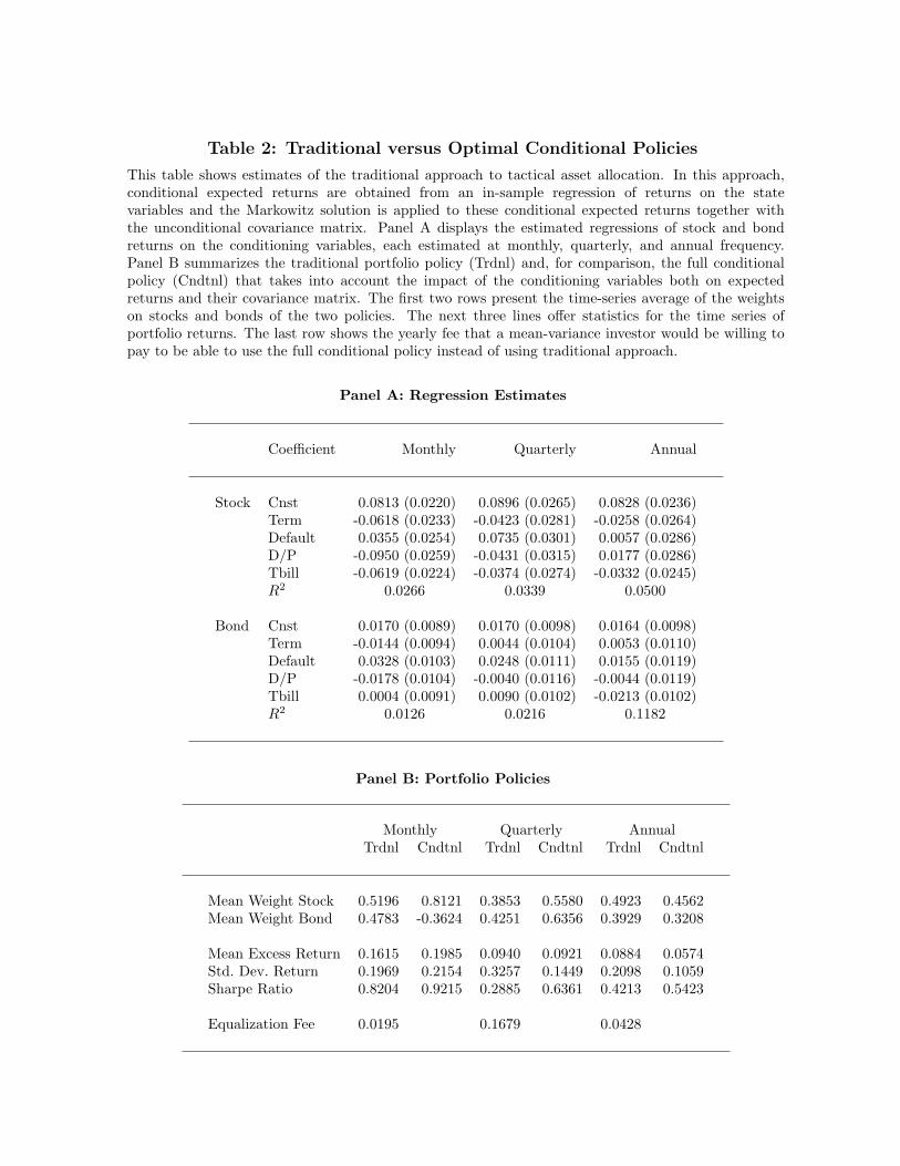
Table 2: Traditional versus Optimal Conditional Policies
This table shows estimates of the traditional approach to tactical asset allocation. In this approach,conditional expected returns are obtained from an in-sample regression of returns on the statevariables and the Markowitz solution is applied to these conditional expected returns together withthe unconditional covariance matrix. Panel A displays the estimated regressions of stock and bondreturns on the conditioning variables, each estimated at monthly, quarterly, and annual frequency.Panel B summarizes the traditional portfolio policy (Trdnl) and, for comparison, the full conditionalpolicy (Cndtnl) that takes into account the impact of the conditioning variables both on expectedreturns and their covariance matrix. The first two rows present the time-series average of the weightson stocks and bonds of the two policies. The next three lines offer statistics for the time series ofportfolio returns. The last row shows the yearly fee that a mean-variance investor would be willing topay to be able to use the full conditional policy instead of using traditional approach.
Panel A: Regression Estimates
Coefficient Monthly Quarterly Annual
Stock Cnst 0.0813 (0.0220) 0.0896 (0.0265) 0.0828 (0.0236)Term -0.0618 (0.0233) -0.0423 (0.0281) -0.0258 (0.0264)Default 0.0355 (0.0254) 0.0735 (0.0301) 0.0057 (0.0286)D/P -0.0950 (0.0259) -0.0431 (0.0315) 0.0177 (0.0286)Tbill -0.0619 (0.0224) -0.0374 (0.0274) -0.0332 (0.0245)R2 0.0266 0.0339 0.0500
Bond Cnst 0.0170 (0.0089) 0.0170 (0.0098) 0.0164 (0.0098)Term -0.0144 (0.0094) 0.0044 (0.0104) 0.0053 (0.0110)Default 0.0328 (0.0103) 0.0248 (0.0111) 0.0155 (0.0119)D/P -0.0178 (0.0104) -0.0040 (0.0116) -0.0044 (0.0119)Tbill 0.0004 (0.0091) 0.0090 (0.0102) -0.0213 (0.0102)R2 0.0126 0.0216 0.1182
Panel B: Portfolio Policies
Monthly Quarterly AnnualTrdnl Cndtnl Trdnl Cndtnl Trdnl Cndtnl
Mean Weight Stock 0.5196 0.8121 0.3853 0.5580 0.4923 0.4562Mean Weight Bond 0.4783 -0.3624 0.4251 0.6356 0.3929 0.3208
Mean Excess Return 0.1615 0.1985 0.0940 0.0921 0.0884 0.0574Std. Dev. Return 0.1969 0.2154 0.3257 0.1449 0.2098 0.1059Sharpe Ratio 0.8204 0.9215 0.2885 0.6361 0.4213 0.5423
Equalization Fee 0.0195 0.1679 0.0428
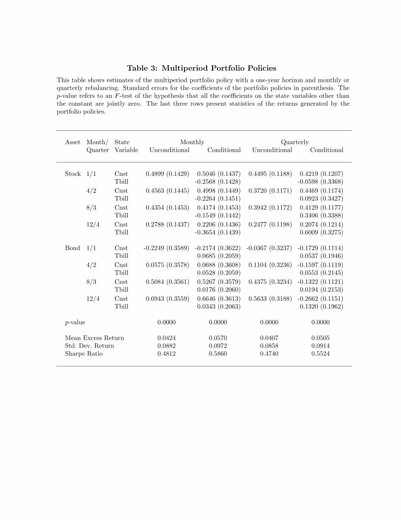
Table 3: Multiperiod Portfolio Policies
This table shows estimates of the multiperiod portfolio policy with a one-year horizon and monthly orquarterly rebalancing. Standard errors for the coefficients of the portfolio policies in parenthesis. Thep-value refers to an F -test of the hypothesis that all the coefficients on the state variables other thanthe constant are jointly zero. The last three rows present statistics of the returns generated by theportfolio policies.
Asset Month/ State Monthly QuarterlyQuarter Variable Unconditional Conditional Unconditional Conditional
Stock 1/1 Cnst 0.4899 (0.1429) 0.5046 (0.1437) 0.4495 (0.1188) 0.4219 (0.1207)Tbill -0.2568 (0.1428) -0.0598 (0.3368)
4/2 Cnst 0.4563 (0.1445) 0.4998 (0.1449) 0.3720 (0.1171) 0.4469 (0.1174)Tbill -0.2264 (0.1451) 0.0923 (0.3427)
8/3 Cnst 0.4354 (0.1453) 0.4174 (0.1453) 0.3942 (0.1172) 0.4129 (0.1177)Tbill -0.1549 (0.1442) 0.3406 (0.3388)
12/4 Cnst 0.2788 (0.1437) 0.2206 (0.1436) 0.2477 (0.1198) 0.2074 (0.1214)Tbill -0.3654 (0.1439) 0.6009 (0.3275)
Bond 1/1 Cnst -0.2249 (0.3589) -0.2174 (0.3622) -0.0367 (0.3237) -0.1729 (0.1114)Tbill 0.0685 (0.2059) 0.0537 (0.1946)
4/2 Cnst 0.0575 (0.3578) 0.0688 (0.3608) 0.1104 (0.3236) -0.1597 (0.1119)Tbill 0.0528 (0.2059) 0.0553 (0.2145)
8/3 Cnst 0.5084 (0.3561) 0.5267 (0.3579) 0.4375 (0.3234) -0.1322 (0.1121)Tbill 0.0176 (0.2060) 0.0194 (0.2153)
12/4 Cnst 0.6943 (0.3559) 0.6646 (0.3613) 0.5633 (0.3188) -0.2662 (0.1151)Tbill 0.0343 (0.2063) 0.1320 (0.1962)
p-value 0.0000 0.0000 0.0000 0.0000
Mean Excess Return 0.0424 0.0570 0.0407 0.0505Std. Dev. Return 0.0882 0.0972 0.0858 0.0914Sharpe Ratio 0.4812 0.5860 0.4740 0.5524

Figure 1: Portfolio Weights of Conditional and Unconditional Policies
This figure displays the time series of conditional portfolio weights. The solid line corresponds to theportfolio weight on the stock and the dash-dotted line corresponds to the portfolio weight on the bond.The constant portfolio weights from the unconditional policy are depicted as straight lines.
1930 1940 1950 1960 1970 1980 1990 2000−5
0
5
10Monthly Rebalancing
Port
folio
Wei
ghts
1930 1940 1950 1960 1970 1980 1990 2000−2
0
2
4
6Quarterly Rebalancing
Port
folio
Wei
ghts
1930 1940 1950 1960 1970 1980 1990 2000
−1
0
1
2
Annual Rebalancing
Year
Port
folio
Wei
ghts

Figure 2: Portfolio Weights of Conditional and Regression-Based Policies
This figure displays the time series of the portfolio weight on the stock obtained from the conditionalapproach as solid line and from the regression-based approach as dashed line. In the regression-basedapproach, conditional expected returns are computed from an in-sample regression of returns on thestate variables, and the Markowitz solution is applied to these conditional expected returns togetherwith the unconditional covariance matrix.
1930 1940 1950 1960 1970 1980 1990 2000−5
0
5
10Monthly Rebalancing
Port
folio
Wei
ghts
1930 1940 1950 1960 1970 1980 1990 2000−2
0
2
4
6Quarterly Rebalancing
Port
folio
Wei
ghts
1930 1940 1950 1960 1970 1980 1990 2000
−1
0
1
2
Annual Rebalancing
Year
Port
folio
Wei
ghts


