Download - Dynamic Programming1 Modified by: Daniel Gomez-Prado, University of Massachusetts Amherst

Dynamic Programming 1
Dynamic Programming
Modified by: Daniel Gomez-Prado, University of Massachusetts Amherst

Dynamic Programming 2
Outline and Reading
Fuzzy Explanation of Dynamic ProgrammingIntroductory example: Matrix Chain-Product (§5.3.1) The General Technique (§5.3.2)A very good example: 0-1 Knapsack Problem (§5.3.3)

Dynamic Programming 3
Matrix Chain-ProductsDynamic Programming is a general algorithm design paradigm.
Rather than give the general structure, let us first give a motivating example:
Matrix Chain-Products
Review: Matrix Multiplication. C = A*B A is d × e and B is e × f
O(def ) timeA C
B
d d
f
e
f
e
i
j
i,j
1
0
],[*],[],[e
k
jkBkiAjiC

Dynamic Programming 4
Matrix Chain-ProductsMatrix Chain-Product: Compute A=A0*A1*…*An-1
Ai is di × di+1
Problem: How to parenthesize?
Example B is 3 × 100 C is 100 × 5 D is 5 × 5 (B*C)*D takes 1500 + 75 = 1575 ops B*(C*D) takes 1500 + 2500 = 4000
ops

Dynamic Programming 5
An Enumeration ApproachMatrix Chain-Product Alg.: Try all possible ways to parenthesize
A=A0*A1*…*An-1
Calculate number of ops for each one Pick the one that is best
Running time: The number of paranethesizations is
equal to the number of binary trees with n nodes
This is exponential! It is called the Catalan number, and it
is almost 4n. This is a terrible algorithm!

Dynamic Programming 6
A Greedy ApproachIdea #1: repeatedly select the product that uses (up) the most operations.Counter-example: A is 10 × 5 B is 5 × 10 C is 10 × 5 D is 5 × 10 Greedy idea #1 gives (A*B)*(C*D), which
takes 500+1000+500 = 2000 ops But A*((B*C)*D) takes 500+250+250 = 1000
ops

Dynamic Programming 7
Another Greedy ApproachIdea #2: repeatedly select the product that uses the fewest operations.Counter-example: A is 101 × 11 B is 11 × 9 C is 9 × 100 D is 100 × 99 Greedy idea #2 gives A*((B*C)*D)), which takes
109989+9900+108900=228789 ops (A*B)*(C*D) takes 9999+89991+89100=189090
ops
The greedy approach is not giving us the optimal value.

Dynamic Programming 8
A “Recursive” Approach
Define subproblems: Find the best parenthesization of Ai*Ai+1*…*Aj. Let Ni,j denote the number of operations done by this
subproblem. The optimal solution for the whole problem is N0,n-1.
Subproblem optimality: The optimal solution can be defined in terms of optimal subproblems
There has to be a final multiplication (root of the expression tree) for the optimal solution.
Say, the final multiply is at index i: (A0*…*Ai)*(Ai+1*…*An-1). Then the optimal solution N0,n-1 is the sum of two optimal
subproblems, N0,i and Ni+1,n-1 plus the time for the last multiply.
If the global optimum did not have these optimal subproblems, we could define an even better “optimal” solution.

Dynamic Programming 9
A Characterizing Equation
The global optimal has to be defined in terms of optimal subproblems, depending on where the final multiply is at.Let us consider all possible places for that final multiply:
Recall that Ai is a di × di+1 dimensional matrix. So, a characterizing equation for Ni,j is the following:
Note that subproblems are not independent--the subproblems overlap.
}{min 11,1,, jkijkki
jkiji dddNNN

Dynamic Programming 11
A Dynamic Programming AlgorithmSince subproblems overlap, we don’t use recursion.Instead, we construct optimal subproblems “bottom-up.” Ni,i’s are easy, so start with themThen do length 2,3,… subproblems, and so on.Running time: O(n3)
Algorithm matrixChain(S):Input: sequence S of n matrices to be multipliedOutput: number of operations in an optimal
paranethization of Sfor i 1 to n-1 do
Ni,i 0 for b 1 to n-1 do
for i 0 to n-b-1 doj i+b
Ni,j +infinityfor k i to j-1 do
Ni,j min{Ni,j , Ni,k +Nk+1,j +di dk+1
dj+1}

Dynamic Programming 12
answerN 0 1
0
1
2 …
n-1
…
n-1j
i
A Dynamic Programming Algorithm VisualizationThe bottom-up construction fills in the N array by diagonalsNi,j gets values from pervious entries in i-th row and j-th column Filling in each entry in the N table takes O(n) time.Total run time: O(n3)Getting actual parenthesization can be done by remembering “k” for each N entry
}{min 11,1,, jkijkki
jkiji dddNNN

Dynamic Programming 13
Matrix Chain algorithmAlgorithm matrixChain(S):
Input: sequence S of n matrices to be multiplied
Output: # of multiplications in optimalparenthesization of S
for i 0 to n-1 do
Ni,i 0 for b 1 to n-1 do // b is # of ops in S
for i 0 to n-b-1 doj i+b
Ni,j +infinityfor k i to j-1 do
sum = Ni,k +Nk+1,j +di dk+1 dj+1
if (sum < Ni,j) then
Ni,j sum
Oi,j k
return N0,n-1
Example: ABCD A is 10 × 5 B is 5 × 10 C is 10 × 5 D is 5 × 10
N 0 1 2 3
0
1
2
3
0
0
0
0
A
B
C
D
AB
BC
CD
A(BC)
(BC)D
(A(BC))D
500
250
500
500
500
10000 0 2
0 1
0

Dynamic Programming 14
Recovering operationsExample: ABCD
A is 10 × 5 B is 5 × 10 C is 10 × 5 D is 5 × 10
N 0 1 2 3
0
1
2
3
0
0
0
0
A
B
C
D
AB
BC
CD
A(BC)
(BC)D
(A(BC))D
500
250
500
500
500
10000 0 2
0 1
0
// return expression for multiplying// matrix chain Ai through Aj
exp(i,j)if (i=j) then // base case, 1 matrix
return ‘Ai’else
k = O[i,j] // see red values on leftS1 = exp(i,k) // 2 recursive calls
S2 = exp(k+1,j)return ‘(‘ S1 S2 ‘)’

Dynamic Programming 15
The General Dynamic Programming Technique
Applies to a problem that at first seems to require a lot of time (possibly exponential), provided we have: Simple subproblems: the subproblems can be
defined in terms of a few variables, such as j, k, l, m, and so on.
Subproblem optimality: the global optimum value can be defined in terms of optimal subproblems
Subproblem overlap: the subproblems are not independent, but instead they overlap (hence, should be constructed bottom-up).
Dynamic Programming 16
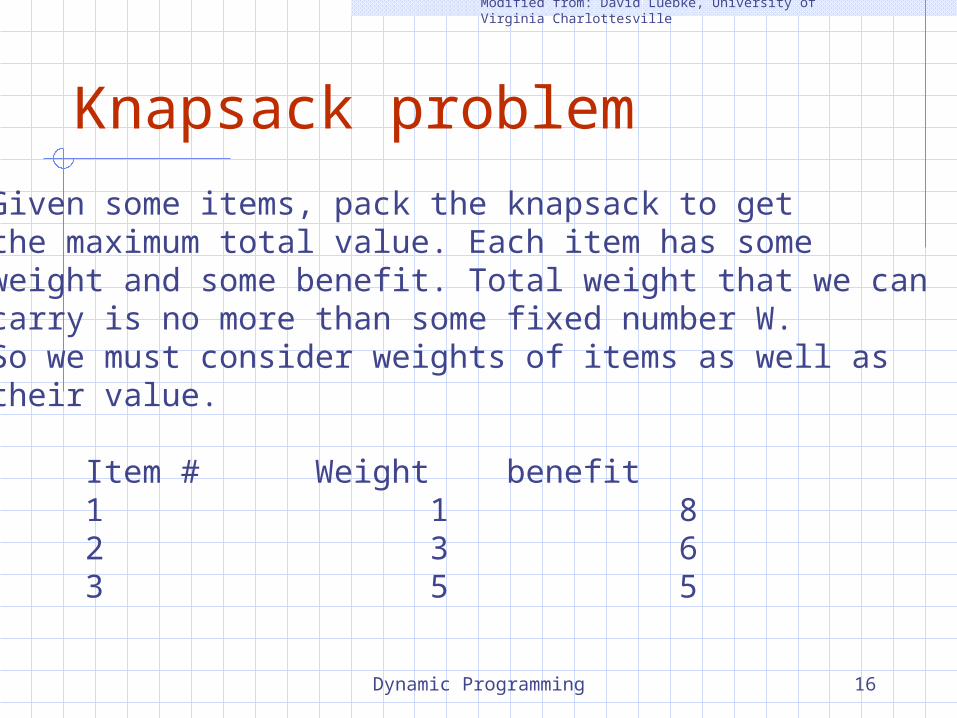
Knapsack problem
Given some items, pack the knapsack to get the maximum total value. Each item has some weight and some benefit. Total weight that we can carry is no more than some fixed number W.So we must consider weights of items as well as their value.
Item # Weight benefit 1 1 8 2 3 6 3 5 5
Modified from: David Luebke, University of Virginia Charlottesville

Dynamic Programming 17
Knapsack problemThere are two versions of the problem:
“0-1 knapsack problem” Items are indivisible; you either take an
item or not. Solved with dynamic programming.
“Fractional knapsack problem” Items are divisible: you can take any
fraction of an item. Solved with a greedy algorithm.
Modified from: David Luebke, University of Virginia Charlottesville

Dynamic Programming 18
The 0/1 Knapsack ProblemGiven: A set S of n items, with each item i having
bi - a positive benefit wi - a positive weight
Goal: Choose items with maximum total benefit but with weight at most W.If we are not allowed to take fractional amounts, then this is the 0/1 knapsack problem.
In this case, we let T denote the set of items we take
Objective: maximize
Constraint:
Ti
ib
Ti
i Ww

Dynamic Programming 19
0-1 Knapsack problem:a picture
W = 20
wi
bi
109
85
54
43
32
Weight Benefit
This is a knapsackMax weight: W = 20
Items
Modified from: David Luebke, University of Virginia Charlottesville

Dynamic Programming 20
0-1 Knapsack problem: brute-force approach
Let’s first solve this problem with a straightforward algorithm
Since there are n items, there are 2n possible combinations of items.We go through all combinations and find the one with the most total value and with total weight less or equal to WRunning time will be O(2n)
Modified from: David Luebke, University of Virginia Charlottesville

Dynamic Programming 21
0-1 Knapsack problem: brute-force approach
Can we do better? Yes, with an algorithm based on dynamic programmingWe need to carefully identify the subproblems
Let’s try this:If items are labeled 1..n, then a subproblem would be to find an optimal solution for Sk = {items labeled 1, 2, .. k}
Modified from: David Luebke, University of Virginia Charlottesville

Dynamic Programming 22
Defining a Subproblem If items are labeled 1..n, then a subproblem
would be to find an optimal solution for Sk = {items labeled 1, 2, .. k}
This is a valid subproblem definition.
The question is: can we describe the final solution (Sn ) in terms of subproblems (Sk)?
Unfortunately, we can’t do that. Explanation follows….
Modified from: David Luebke, University of Virginia Charlottesville

Dynamic Programming 23
Defining a Subproblem
Max weight: W = 20For S4:Total weight: 14;Total benefit: 20
w1 =2
b1 =3
w2 =4
b2 =5
w3 =5
b3 =8
w4 =3
b4 =4 wi bi
10
85
54
43
32
Weight Benefit
9
Item
#
4
3
2
1
5
S4
S5
w1 =2
b1 =3
w2 =4
b2 =5
w3 =5
b3 =8
w4 =9
b4 =10
For S5:Total weight: 20Total benefit: 26
Solution for S4 is not part of the solution for S5!!!
Modified from: David Luebke, University of Virginia Charlottesville

Dynamic Programming 24
Defining a Subproblem (continued)
As we have seen, the solution for S4 is not part of the solution for S5
So our definition of a subproblem is flawed and we need another one!Let’s add another parameter: w, which will represent the exact weight for each subset of itemsThe subproblem then will be to compute B[k,w]
Modified from: David Luebke, University of Virginia Charlottesville

Dynamic Programming 25
Recursive Formula for subproblems
It means, that the best subset of Sk that has total weight w is one of the two: the best subset of Sk-1 that has total
weight w, or the best subset of Sk-1 that has total
weight w-wk plus the item k
else }],1[],,1[max{
if ],1[],[
kk
k
bwwkBwkB
wwwkBwkB
Recursive formula for subproblems:
Modified from: David Luebke, University of Virginia Charlottesville

Dynamic Programming 26
Recursive Formula
The best subset of Sk that has the total weight w, either contains item k or not.First case: wk>w. Item k can’t be part of the solution, since if it was, the total weight would be > w, which is unacceptableSecond case: wk <=w. Then the item k can be in the solution, and we choose the case with greater value
else }],1[],,1[max{
if ],1[],[
kk
k
bwwkBwkB
wwwkBwkB
Modified from: David Luebke, University of Virginia Charlottesville

Dynamic Programming 27
0-1 Knapsack Algorithmfor w = 0 to W
B[0,w] = 0for i = 0 to n
B[i,0] = 0for w = 0 to W
if wi <= w // item “i” can be part of the solution
if bi + B[i-1,w-wi] > B[i-1,w]
B[i,w] = bi + B[i-1,w- wi]
elseB[i,w] = B[i-1,w]
else B[i,w] = B[i-1,w] // wi > w
Modified from: David Luebke, University of Virginia Charlottesville
<the rest of the code>
What is the running time of this algorithm?
O(W)
O(W)
Repeat n times
O(n*W)
Remember that the brute-force algorithm takes O(2n)
i
w
B[i,w]B[i-1,w]
B[i-1,w-wi]

Dynamic Programming 28
Example
Let’s run our algorithm on the following data:
n = 4 (# of elements)W = 5 (max weight)
Elements (weight, benefit):(2,3), (3,4), (4,5), (5,6)
Modified from: David Luebke, University of Virginia Charlottesville

Dynamic Programming 29
Example (continue)
for w = 0 to WB[0,w] = 0
0
0
0
0
0
0
W0
1
2
3
4
5
i 0 1 2 3
4
Modified from: David Luebke, University of Virginia Charlottesville

Dynamic Programming 30
Example (continue)
for i = 0 to nB[i,0] = 0
0
0
0
0
0
0
W0
1
2
3
4
5
i 0 1 2 3
0 0 0 0
4
Modified from: David Luebke, University of Virginia Charlottesville

Dynamic Programming 31
Example (continue)
if wi <= w // item i can be part of the solution if bi + B[i-1,w-wi] > B[i-1,w] B[i,w] = bi + B[i-1,w- wi] else B[i,w] = B[i-1,w] else B[i,w] = B[i-1,w] // wi > w
0
0
0
0
0
0
W0
1
2
3
4
5
i 0 1 2 3
0 0 0 0i=1bi=3
wi=2
w=1w-wi =-1
Items:1: (2,3)2: (3,4)3: (4,5) 4: (5,6)
4
0
Modified from: David Luebke, University of Virginia Charlottesville

Dynamic Programming 32
Example (continue)
if wi <= w // item i can be part of the solution if bi + B[i-1,w-wi] > B[i-1,w] B[i,w] = bi + B[i-1,w- wi] else B[i,w] = B[i-1,w] else B[i,w] = B[i-1,w] // wi > w
0
0
0
0
0
0
W0
1
2
3
4
5
i 0 1 2 3
0 0 0 0i=1bi=3
wi=2
w=2w-wi =0
Items:1: (2,3)2: (3,4)3: (4,5) 4: (5,6)
4
0
3
Modified from: David Luebke, University of Virginia Charlottesville

Dynamic Programming 33
Example (continue)
if wi <= w // item i can be part of the solution if bi + B[i-1,w-wi] > B[i-1,w] B[i,w] = bi + B[i-1,w- wi] else B[i,w] = B[i-1,w]
else B[i,w] = B[i-1,w] // wi > w
0
0
0
0
0
0
W0
1
2
3
4
5
i 0 1 2 3
0 0 0 0i=1bi=3
wi=2
w=3w-wi=1
Items:1: (2,3)2: (3,4)3: (4,5) 4: (5,6)
4
0
3
3
Modified from: David Luebke, University of Virginia Charlottesville

Dynamic Programming 34
Example (continue)
if wi <= w // item i can be part of the solution if bi + B[i-1,w-wi] > B[i-1,w] B[i,w] = bi + B[i-1,w- wi] else B[i,w] = B[i-1,w]
else B[i,w] = B[i-1,w] // wi > w
0
0
0
0
0
0
W0
1
2
3
4
5
i 0 1 2 3
0 0 0 0i=1bi=3
wi=2
w=4w-wi=2
Items:1: (2,3)2: (3,4)3: (4,5) 4: (5,6)
4
0
3
3
3
Modified from: David Luebke, University of Virginia Charlottesville

Dynamic Programming 35
Example (continue)
if wi <= w // item i can be part of the solution if bi + B[i-1,w-wi] > B[i-1,w] B[i,w] = bi + B[i-1,w- wi] else B[i,w] = B[i-1,w]
else B[i,w] = B[i-1,w] // wi > w
0
0
0
0
0
0
W0
1
2
3
4
5
i 0 1 2 3
0 0 0 0i=1bi=3
wi=2
w=5w-wi=2
Items:1: (2,3)2: (3,4)3: (4,5) 4: (5,6)
4
0
3
3
3
3
Modified from: David Luebke, University of Virginia Charlottesville

Dynamic Programming 36
Example (continue)
if wi <= w // item i can be part of the solution if bi + B[i-1,w-wi] > B[i-1,w] B[i,w] = bi + B[i-1,w- wi] else B[i,w] = B[i-1,w] else B[i,w] = B[i-1,w] // wi > w
0
0
0
0
0
0
W0
1
2
3
4
5
i 0 1 2 3
0 0 0 0i=2bi=4
wi=3
w=1w-wi=-2
Items:1: (2,3)2: (3,4)3: (4,5) 4: (5,6)
4
0
3
3
3
3
0
Modified from: David Luebke, University of Virginia Charlottesville

Dynamic Programming 37
Example (continue)
if wi <= w // item i can be part of the solution if bi + B[i-1,w-wi] > B[i-1,w] B[i,w] = bi + B[i-1,w- wi] else B[i,w] = B[i-1,w]
else B[i,w] = B[i-1,w] // wi > w
0
0
0
0
0
0
W0
1
2
3
4
5
i 0 1 2 3
0 0 0 0i=2bi=4
wi=3
w=2w-wi=-1
Items:1: (2,3)2: (3,4)3: (4,5) 4: (5,6)
4
0
3
3
3
3
0
3
Modified from: David Luebke, University of Virginia Charlottesville

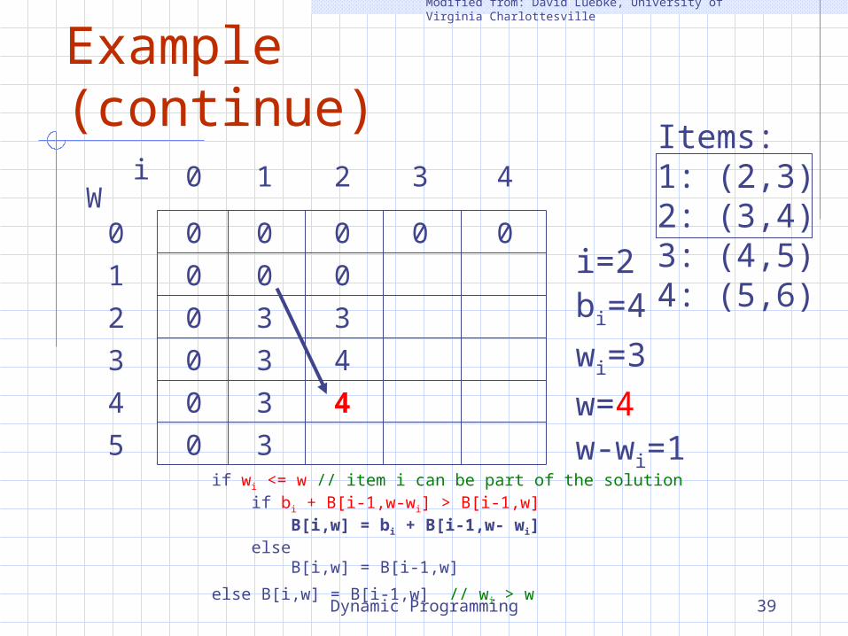
Dynamic Programming 38
if wi <= w // item i can be part of the solution if bi + B[i-1,w-wi] > B[i-1,w] B[i,w] = bi + B[i-1,w- wi] else B[i,w] = B[i-1,w]
else B[i,w] = B[i-1,w] // wi > w
0
0
0
0
0
0
W0
1
2
3
4
5
i 0 1 2 3
0 0 0 0i=2bi=4
wi=3
w=3w-wi=0
Items:1: (2,3)2: (3,4)3: (4,5) 4: (5,6)
4
0
3
3
3
3
0
3
4
Modified from: David Luebke, University of Virginia Charlottesville
Example (continue)
Dynamic Programming 39
if wi <= w // item i can be part of the solution if bi + B[i-1,w-wi] > B[i-1,w] B[i,w] = bi + B[i-1,w- wi] else B[i,w] = B[i-1,w]
else B[i,w] = B[i-1,w] // wi > w
0
0
0
0
0
0
W0
1
2
3
4
5
i 0 1 2 3
0 0 0 0i=2bi=4
wi=3
w=4w-wi=1
Items:1: (2,3)2: (3,4)3: (4,5) 4: (5,6)
4
0
3
3
3
3
0
3
4
4
Modified from: David Luebke, University of Virginia Charlottesville
Example (continue)

Dynamic Programming 40
if wi <= w // item i can be part of the solution if bi + B[i-1,w-wi] > B[i-1,w] B[i,w] = bi + B[i-1,w- wi] else B[i,w] = B[i-1,w]
else B[i,w] = B[i-1,w] // wi > w
0
0
0
0
0
0
W0
1
2
3
4
5
i 0 1 2 3
0 0 0 0i=2bi=4
wi=3
w=5w-wi=2
Items:1: (2,3)2: (3,4)3: (4,5) 4: (5,6)
4
0
3
3
3
3
0
3
4
4
7
Modified from: David Luebke, University of Virginia Charlottesville
Example (continue)

Dynamic Programming 41
if wi <= w // item i can be part of the solution if bi + B[i-1,w-wi] > B[i-1,w] B[i,w] = bi + B[i-1,w- wi] else B[i,w] = B[i-1,w]
else B[i,w] = B[i-1,w] // wi > w
0
0
0
0
0
0
W0
1
2
3
4
5
i 0 1 2 3
0 0 0 0i=3bi=5
wi=4
w=1..3
Items:1: (2,3)2: (3,4)3: (4,5) 4: (5,6)
4
0
3
3
3
3
00
3
4
4
7
0
3
4
Modified from: David Luebke, University of Virginia Charlottesville
Example (continue)

Dynamic Programming 42
if wi <= w // item i can be part of the solution if bi + B[i-1,w-wi] > B[i-1,w] B[i,w] = bi + B[i-1,w- wi] else B[i,w] = B[i-1,w] else B[i,w] = B[i-1,w] // wi > w
0
0
0
0
0
0
W0
1
2
3
4
5
i 0 1 2 3
0 0 0 0i=3bi=5
wi=4
w=4w- wi=0
Items:1: (2,3)2: (3,4)3: (4,5) 4: (5,6)
4
0 00
3
4
4
7
0
3
4
5
3
3
3
3
Modified from: David Luebke, University of Virginia Charlottesville
Example (continue)

Dynamic Programming 43
if wi <= w // item i can be part of the solution if bi + B[i-1,w-wi] > B[i-1,w] B[i,w] = bi + B[i-1,w- wi] else B[i,w] = B[i-1,w] else B[i,w] = B[i-1,w] // wi > w
0
0
0
0
0
0
W0
1
2
3
4
5
i 0 1 2 3
0 0 0 0i=3bi=5
wi=4
w=5w- wi=1
Items:1: (2,3)2: (3,4)3: (4,5) 4: (5,6)
4
0 00
3
4
4
7
0
3
4
5
7
3
3
3
3
Modified from: David Luebke, University of Virginia Charlottesville
Example (continue)

Dynamic Programming 44
if wi <= w // item i can be part of the solution if bi + B[i-1,w-wi] > B[i-1,w] B[i,w] = bi + B[i-1,w- wi] else B[i,w] = B[i-1,w]
else B[i,w] = B[i-1,w] // wi > w
0
0
0
0
0
0
W0
1
2
3
4
5
i 0 1 2 3
0 0 0 0i=3bi=5
wi=4
w=1..4
Items:1: (2,3)2: (3,4)3: (4,5) 4: (5,6)
4
0 00
3
4
4
7
0
3
4
5
7
0
3
4
5
3
3
3
3
Modified from: David Luebke, University of Virginia Charlottesville
Example (continue)

Dynamic Programming 45
if wi <= w // item i can be part of the solution if bi + B[i-1,w-wi] > B[i-1,w] B[i,w] = bi + B[i-1,w- wi] else B[i,w] = B[i-1,w]
else B[i,w] = B[i-1,w] // wi > w
0
0
0
0
0
0
W0
1
2
3
4
5
i 0 1 2 3
0 0 0 0i=3bi=5
wi=4
w=5
Items:1: (2,3)2: (3,4)3: (4,5) 4: (5,6)
4
0 00
3
4
4
7
0
3
4
5
7
0
3
4
5
7
3
3
3
3
Modified from: David Luebke, University of Virginia Charlottesville
Example (continue)

Dynamic Programming 46
Comments
This algorithm only finds the max possible value that can be carried in the knapsack
To know the items that make this maximum value, an addition to this algorithm is necessary
Modified from: David Luebke, University of Virginia Charlottesville

Dynamic Programming 47
How to find actual knapsack items
All of the information we need is in the table. B[n,W] is the maximal value of items that can be placed in the Knapsack.Let i=n and k=Wif B[i,k] ≠ B[i -1,k] then
mark the ith item as in the knapsacki = i -1, k = k-wi
elsei = i -1 // Assume the ith item is not in the knapsack// Could it be in the optimally packed knapsack?
Modified from: David Luebke, University of Virginia Charlottesville

Dynamic Programming 48
i = n , k = w while i , k > 0 if B[i,k] ≠ B[i-1,k] mark the ith item as the knapsack i = i-1, k = k-wi
else i = i-1
0
0
0
0
0
0
W0
1
2
3
4
5
i 0 1 2 3
0 0 0 0i=4k=5bi=5
wi=6
B[i,k]=7B[i-1,k]=7
Items:1: (2,3)2: (3,4)3: (4,5) 4: (5,6)
4
0 00
3
4
4
7
0
3
4
5
7
0
3
4
5
7
3
3
3
3
Modified from: David Luebke, University of Virginia Charlottesville
Finding Items (continue)

Dynamic Programming 49
i = n , k = w while i , k > 0 if B[i,k] ≠ B[i-1,k] mark the ith item as the knapsack i = i-1, k = k-wi
else i = i-1
0
0
0
0
0
0
W0
1
2
3
4
5
i 0 1 2 3
0 0 0 0i=4k=5bi=5
wi=6
B[i,k]=7B[i-1,k]=7
Items:1: (2,3)2: (3,4)3: (4,5) 4: (5,6)
4
0 00
3
4
4
7
0
3
4
5
7
0
3
4
5
7
3
3
3
3
Modified from: David Luebke, University of Virginia Charlottesville
Finding Items (continue)

Dynamic Programming 50
i = n , k = w while i , k > 0 if B[i,k] ≠ B[i-1,k] mark the ith item as the knapsack i = i-1, k = k-wi
else i = i-1
0
0
0
0
0
0
W0
1
2
3
4
5
i 0 1 2 3
0 0 0 0i=3k=5bi=5
wi=4
B[i,k]=7B[i-1,k]=7
Items:1: (2,3)2: (3,4)3: (4,5) 4: (5,6)
4
0 00
3
4
4
7
0
3
4
5
7
0
3
4
5
7
3
3
3
3
Modified from: David Luebke, University of Virginia Charlottesville
Finding Items (continue)

Dynamic Programming 51
i = n , k = w while i , k > 0 if B[i,k] ≠ B[i-1,k] mark the ith item as the knapsack i = i-1, k = k-wi
else i = i-1
0
0
0
0
0
0
W0
1
2
3
4
5
i 0 1 2 3
0 0 0 0i=2k=5bi=4
wi=3
B[i,k]=7B[i-1,k]=3k-wi=2
Items:1: (2,3)2: (3,4)3: (4,5) 4: (5,6)
4
0 00
3
4
4
7
0
3
4
5
7
0
3
4
5
7
3
3
3
3
Modified from: David Luebke, University of Virginia Charlottesville
Finding Items (continue)

Dynamic Programming 52
i = n , k = w while i , k > 0 if B[i,k] ≠ B[i-1,k] mark the ith item as the knapsack i = i-1, k = k-wi
else i = i-1
0
0
0
0
0
0
W0
1
2
3
4
5
i 0 1 2 3
0 0 0 0i=1k=2bi=3
wi=2
B[i,k]=3B[i-1,k]=0k-wi=0
Items:1: (2,3)2: (3,4)3: (4,5) 4: (5,6)
4
0 00
3
4
4
7
0
3
4
5
7
0
3
4
5
7
3
3
3
3
Modified from: David Luebke, University of Virginia Charlottesville
Finding Items (continue)

Dynamic Programming 53
i = n , k = w while i , k > 0 if B[i,k] ≠ B[i-1,k] mark the ith item as the knapsack i = i-1, k = k-wi
else i = i-1
0
0
0
0
0
0
W0
1
2
3
4
5
i 0 1 2 3
0 0 0 0i=0k=0
Items:1: (2,3)2: (3,4)3: (4,5) 4: (5,6)
4
0 00
3
4
4
7
0
3
4
5
7
0
3
4
5
7
3
3
3
3
Modified from: David Luebke, University of Virginia Charlottesville
Finding Items (continue)
The optimal knapsackshould contain items:
{ 1 , 2 }

Dynamic Programming 54
i = n , k = w while i , k > 0 if B[i,k] ≠ B[i-1,k] mark the ith item as the knapsack i = i-1, k = k-wi
else i = i-1
0
0
0
0
0
0
W0
1
2
3
4
5
i 0 1 2 3
0 0 0 0i=0k=0
Items:1: (2,3)2: (3,4)3: (4,5) 4: (5,6)
4
0 00
3
4
4
7
0
3
4
5
7
0
3
4
5
7
3
3
3
3
Modified from: David Luebke, University of Virginia Charlottesville
Finding Items (continue)
The optimal knapsackshould contain items:
{ 1 , 2 }

Dynamic Programming 55
Conclusions
Dynamic programming is a useful technique for solving certain kind of problemsWhen the solution can be recursively described in terms of partial solutions, we can store these partial solutions and re-use them as necessaryRunning time of dynamic programming algorithm vs. naïve algorithm:» 0-1 Knapsack problem: O(W*n) vs. O(2n)
Modified from: David Luebke, University of Virginia Charlottesville

Dynamic Programming 56
RememberHw #2 is already posted. It is due on the day of the Exam.
Midterm Exam is scheduled for Monday, March 28 at 5:30 pm or later.
There is a mandatory seminar for CSE student on Monday, March 28, at 4:00, hence we cannot start the exam earlier than 5:30 pm.


