
copy 2016 CY Lin Columbia UniversityE6893 Big Data Analytics ndash Lecture 9 Linked Big Data Graph Computing
E6893 Big Data Analytics Lecture 9
Linked Big Data mdash Graphical Models (II)
Ching-Yung Lin PhD
Adjunct Professor Dept of Electrical Engineering and Computer Science
November 2nd 2016
copy 2016 CY Lin Columbia UniversityE6893 Big Data Analytics ndash Lecture 9 Linked Big Data Graph Computing2
Outline
bull Overview and Background
bull Bayesian Network and Inference
bull Node level parallelism and computation kernels
bull Architecture-aware structural parallelism and scheduling
bull Conclusion
Thanks to Dr Yinglong Xiarsquos contributions
copy 2016 CY Lin Columbia UniversityE6893 Big Data Analytics ndash Lecture 9 Linked Big Data Graph Computing3
Big Data Analytics and High Performance Computing
bull Big Data Analytics ndash Widespread impact ndash Rapidly increasing volume of data ndash Real time requirement ndash Growing demanding for High
Performance Computing algorithms
bull High Performance Computing ndash Parallel computing capability at
various scales ndash Multicore is the de facto standard ndash From multi-many-core to clusters ndash Accelerate Big Data analytics
Anomaly detection
Ecology Market
Analysis
Social Tie Discovery
Business Data Mining
Rec
omm
enda
tion
Behavior prediction
Twitter has 340 million tweets and 16 billion queries a day from 140 million users
BlueGeneQ Sequoia has 16 million cores offering 20 PFlops ranked 1 in TOP500
copy 2016 CY Lin Columbia UniversityE6893 Big Data Analytics ndash Lecture 9 Linked Big Data Graph Computing45
Example Graph Sizes and Graph Capacity
Scale
Throughput
100T
10P
Scale is the number of nodes in a graph assuming the node degree is 25 the average degree in Facebook
Throughput isthe tera-number of computationstaking place ina second
100P
1E
10G 100G 1T 1P1G
copy 2016 CY Lin Columbia UniversityE6893 Big Data Analytics ndash Lecture 9 Linked Big Data Graph Computing5
Challenges ndash Graph Analytic Optimization based on Hardware Platforms
Development productivity vs System performance ndash High level developers rarr limited knowledge on system architectures ndash Not consider platform architectures rarr difficult to achieve high performance
Performance optimization requires tremendous knowledge on system architectures Optimization strategies vary significantly from one graph workload type to another
Multicore rarr Mutex locks for synchronization possible false sharing in cache data collaboration between threads
Manycore rarr high computation capability but also possibly high coordination overhead
Heterogeneous capacity of cores of systems where tasks affiliation is different
High latency in communication among cluster compute nodes
copy 2016 CY Lin Columbia UniversityE6893 Big Data Analytics ndash Lecture 9 Linked Big Data Graph Computing67
Challenges - Input Dependent Computation amp Communication Cost
Understanding computation and commsynchronisation overheads help improve system performance
The ratio is HIGHLY dependent on input graph topology graph property ndash Different algorithms lead to different relationship ndash Even for the same algorithm the input can impact the ratio
Parallel BFS in BSP model CompSync in thread
Blue CompYellow SyncComm
Different input leads to different ratios
copy 2016 CY Lin Columbia UniversityE6893 Big Data Analytics ndash Lecture 9 Linked Big Data Graph Computing7
Graph Workload Traditional (non-graph) computations
Example rarr scientific computations Characteristics
Graph analytic computations Case Study Probabilistic inference in graphical models is a representative ndash (a) Vertices + edges rarr Graph structure ndash (b) Parameters (CPTs) on each node rarr Graph property ndash (c) Changes of graph structure rarr Graph dynamics
Example Matrix A B
Regular memory access Relatively good data locality Computational intensive
Graphical Model Graph + Parameters (Properties) Node rarr Random variables Edge rarr Conditional dependency Parameter rarr Conditional distribution
Inference for anomalous behaviors in a social network
Conditional distribution table (CPT)
copy 2016 CY Lin Columbia UniversityE6893 Big Data Analytics ndash Lecture 9 Linked Big Data Graph Computing8
Graph Workload Types
Type 1 Computations on graph structures topologies Example rarr converting Bayesian network into junction tree graph traversal (BFSDFS) etc Characteristics rarr Poor locality irregular memory access limited numeric operations
Type 2 Computations on graphs with rich properties Example rarr Belief propagation diffuse information through a graph using statistical models Characteristics
Locality and memory access patterndepend on vertex models
Typically a lot of numeric operations Hybrid workload
Type 3 Computations on dynamic graphs Example rarr streaming graph clustering incremental k-core etc Characteristics
Poor locality irregular memory access Operations to update a model (eg cluster sub-graph) Hybrid workload
Bayesian network to Junction tree
3-core subgraph
copy 2016 CY Lin Columbia UniversityE6893 Big Data Analytics ndash Lecture 9 Linked Big Data Graph Computing9
Scheduling on Clusters with Distributed Memory
Necessity for utilizing clusters with distributed memory Increasing capacity of aggregated resources Accelerate computation even though a graph
can fit into a shared memory Generic distributed solution remains a challenge
Optimized partitioning is NP-hard for large graphs especially for dynamic graphs
Graph RDMA enables a virtual shared memory platform Merits rarr remote pointers one-side operation
near wire-speed remote access
The overhead due to remote commutation among 3 mc is very low due to RDMA
Graph RDMA uses key-value queues with remote pointers
copy 2016 CY Lin Columbia UniversityE6893 Big Data Analytics ndash Lecture 9 Linked Big Data Graph Computing10
Explore BlueGene and HMC for Superior Performance BlueGene offers super performance for large scale graph-based applications
4-way 18-core PowerPC x 1024 compute nodes rarr 20 PFLOPS Winner of GRAPH500 (Sequoia LLNL) Exploit RDMA FIFO and PAMI to achieve high performance
Hybrid Memory Cube for Deep Computing Parallelism at 3 levels Data-centric computation Innovative computation
model
Inference in BSP model 0
31
24
Visited
Frontier
New Frontier
Not Reached
Propagate Belief to BN nodes in Frontier
Local comp
converge
Global comm
copy 2016 CY Lin Columbia UniversityE6893 Big Data Analytics ndash Lecture 9 Linked Big Data Graph Computing11
Outline
bull Overview and Background
bull Bayesian Network and Inference
bull Node level parallelism and computation kernels
bull Architecture-aware structural parallelism and scheduling
bull Conclusion
copy 2016 CY Lin Columbia UniversityE6893 Big Data Analytics ndash Lecture 9 Linked Big Data Graph Computing12
Large Scale Graphical Models for Big Data Analytics
Big Data Analytics
Many critical Big Data problems are based on inter-related entities
Typical analysis for Big Data involves reasoning and prediction under uncertainties
Graphical Models (Graph + Probability)
Graph-based representation of conditional independence
Key computations include structure learning and probabilistic inference
11 5 6 TT TF FT FFT 07 03 06 04 F 03 07 04 05
copy 2016 CY Lin Columbia UniversityE6893 Big Data Analytics ndash Lecture 9 Linked Big Data Graph Computing13
Graphical Models for Big Data Analytics
Graphical Models for Big Data
Challenges Problem graph Compact representation Parallelism Target platforms helliphellip
Applications Atmospheric troubleshooting (PNNL) Disease diagnosis (QMR-DT) Anomaly Detection (DARPA) Customer Behavior Prediction helliphellip
Even for this 15-node BN of 5 states for each node the conditional probability distribution table (PDT) for the degree of interest consists of 9765625 entries
Traditional ML or AI graphical models do not scale to thousands of inference nodes
copy 2016 CY Lin Columbia UniversityE6893 Big Data Analytics ndash Lecture 9 Linked Big Data Graph Computing14
Systematic Solution for Parallel Inference
Bayesian network
Junction tree
Evidence Propagation
Posterior probability
of query variables
Output
Parallel Computing PlatformsAccelerate
Inference
Gra
phic
al M
odel
C3 - Identify primitives in probabilistic inference (PDCSrsquo09 Best Paperhellip)
C2 - Parallel conversion of Bayesian Network to Junction
tree (ParCorsquo07)
C3ampC4 - Efficiently map algorithms to HPC architectures (IPDPSrsquo08PDCSrsquo10 Best Paperhelliphellip)
Evidence
Big Data Problems
C1ampC2 ndash Modeling with reduced computation
pressure (PDCSrsquo09 UAIrsquo12)
An
alyt
ics
HP
C
Challenges C1 Problem graph C2 Effective representation C3 Parallelism C4 Target platforms helliphellip
copy 2016 CY Lin Columbia UniversityE6893 Big Data Analytics ndash Lecture 9 Linked Big Data Graph Computing15
Target Platforms
bull Homogeneous multicore processors ndash Intel Xeon E5335 (Clovertown) ndash AMD Opteron 2347 (Barcelona) ndash Netezza (FPGA multicore)
bull Homogeneous manycore processors ndash Sun UltraSPARC T2 (Niagara 2) GPGPU
bull Heterogeneous multicore processors ndash Cell Broadband Engine
bull Clusters ndash HPCC DataStar BlueGene etc
copy 2016 CY Lin Columbia UniversityE6893 Big Data Analytics ndash Lecture 9 Linked Big Data Graph Computing16
Target Platforms (Cont) - What can we learn from the diagrams
What are the differences between thesearchitectures
What are the potential impacts to user programming models
copy 2016 CY Lin Columbia UniversityE6893 Big Data Analytics ndash Lecture 9 Linked Big Data Graph Computing17
Bayesian Network
bull Directed acyclic graph (DAG) + Parameters ndash Random variables dependence and conditional probability tables (CPTs) ndash Compactly model a joint distribution
Compact representation
An old example
copy 2016 CY Lin Columbia UniversityE6893 Big Data Analytics ndash Lecture 9 Linked Big Data Graph Computing18
Question How to Update the Bayesian Network Structure
How to update Bayesian network structure if the sprinkler has a rain sensor Note that the rain sensor can control the sprinkler according to the weather
copy 2016 CY Lin Columbia UniversityE6893 Big Data Analytics ndash Lecture 9 Linked Big Data Graph Computing19
Updated Bayesian Network Structure
Sprinkler is now independent of Cloudy but becomes directly dependent on Rain The structure update results in the new compact
representation of the joint distribution
Cloudy
Rain
WetGrass
Sprinkler
P(C=F) P(C=T) 05 05
C P(C=F) P(C=T) F 08 02 T 02 08
R P(S=F) P(S=T) F 01 09 T 099 001
S R P(W=F) P(W=T) F F 01 09 T F 10 00 F T 01 09 T T 001 099
copy 2016 CY Lin Columbia UniversityE6893 Big Data Analytics ndash Lecture 9 Linked Big Data Graph Computing20
Inference in a Simple Bayesian Network
What is the probability that the grass got wet (W=1) if we know someone used the sprinkler (S=1) and the it did not rain (R=0) Compute or table-lookup
What is the probability that the grass got wet if there is no rain Is there a single answer P(W=1|R=0) Either 00 or 09
What is the probability that the grass got wet P(W=1) Think about the meaning
of the net What is the probability that the
sprinkler is used given the observation of wet grass P(S=1|W=1) Think about the model name
copy 2016 CY Lin Columbia UniversityE6893 Big Data Analytics ndash Lecture 9 Linked Big Data Graph Computing21
Inference on Simple Bayesian Networks (Cont)
What is the probability that the sprinkler is used given the observation of wet grass
Infer p(S=1|W=1)
The joint distribution
How much time does it take for the computation What if the variables are not binary
copy 2016 CY Lin Columbia UniversityE6893 Big Data Analytics ndash Lecture 9 Linked Big Data Graph Computing22
Inference on Large Scale Graphs Example - Atmospheric Radiation Measurement (PNNL)
bull Atmosphere combines measurements of different atmospheric parameters from multiple instruments that can identify unphysical or problematic data bull ARM instruments run unattended 24 hours 7 days a week bull Each site has gt 20 instruments and is measuring hundreds of data variables
4550812 CPT entries 2846 cliques 39 averages states per node
bull Random variables represent climate sensor measurements
bull States for each variable are defined by examining range of and patterns in historical measurement data
bull Links identify highly-correlated measurements as detected by computing the Pearson Correlation across pairs of variables
copy 2016 CY Lin Columbia UniversityE6893 Big Data Analytics ndash Lecture 9 Linked Big Data Graph Computing23
Use Case Smarter another Planet
Goal Atmospheric Radiation Measurement (ARM) climate research facility provides 24x7 continuous field observations of cloud aerosol and radiative processes Graphical models can automate the validation with improvement efficiency and performance
Approach BN is built to represent the dependence among sensors and replicated across timesteps BN parameters are learned from over 15 years of ARM climate data to support distributed climate sensor validation Inference validates sensors in the connected instruments
Bayesian Network 3 timesteps 63 variables 39 avg states 40 avg indegree 16858 CPT entries Junction Tree 67 cliques 873064 PT entries in cliques
Bayesian Network
copy 2016 CY Lin Columbia UniversityE6893 Big Data Analytics ndash Lecture 975
Story ndash Espionage Example
bull Personal stress bull Gender identity confusion
bull Family change (termination of a stable relationship)
bull Job stress bull ndash Dissatisfaction with work
bull Job roles and location (sent to Iraq) bull long work hours (147)
bull Attack
bull Brought music CD to work and downloaded copied documents onto it with his own account
Attack
Personal stress
Planning
Personality
Job stress
Unstable Mental status
Personal event
Job event
bull
bull Unstable Mental Status bull Fight with colleagues write complaining emails to
colleagues
bull Emotional collapse in workspace (crying violence against objects)
bull Large number of unhappy Facebook posts (work-related and emotional)
bull Planning bull Online chat with a hacker confiding his first
attempt of leaking the information
bull
75
copy 2016 CY Lin Columbia UniversityE6893 Big Data Analytics ndash Lecture 9 Linked Big Data Graph Computing25
Behavior Analysis ndash Large Scale Graphical Models
ClientsAccount team
Delivery team
Competitors
Partners
EmailMeeting
hellip
Instant Messaging
Blogging
CSSociology
SNAEE
Sensor
Time
Personal Network Modeling
Channel Modeling
Behavior Evolution Modeling
User behaviors can be observed and analyzed at several levels
Single user BN for detection
Cross-user BN for detection and validation
Demo
copy 2016 CY Lin Columbia UniversityE6893 Big Data Analytics ndash Lecture 977
Example of Graphical Analytics and Provenance
77
Markov Network
Bayesian Network
Latent Network
copy 2016 CY Lin Columbia UniversityE6893 Big Data Analytics ndash Lecture 9 Linked Big Data Graph Computing27
Independency amp Conditional Independence in Bayesian Inference
Three canonical graphs
copy 2016 CY Lin Columbia UniversityE6893 Big Data Analytics ndash Lecture 9 Linked Big Data Graph Computing28
Naiumlve Inference ndash Conditional Independence Determination
A intuitive ldquoreachabilityrdquo algorithm for naiumlve inference - CI query Bayes Ball Algorithm to test CI query
copy 2016 CY Lin Columbia UniversityE6893 Big Data Analytics ndash Lecture 9 Linked Big Data Graph Computing29
From Bayesian Network to Junction Tree ndash Exact Inference
bull Conditional dependence among random variables allows information propagated from a node to another foundation of probabilistic inference
Bayesrsquo theorem can not be applied directly to non-singly connected networks as it would yield erroneous results
Given evidence (observations) E output the posterior probabilities of query P(Q|E)
Therefore junction trees are used to implement exact inference
NP hard
node rarr random variable edge rarr precedence relationship conditional probability table (CPT)
Not straightforward
copy 2016 CY Lin Columbia UniversityE6893 Big Data Analytics ndash Lecture 9 Linked Big Data Graph Computing30
Probabilistic Inference in Junction Tree
bull Inference in junction trees replies on the probabilistic representation of the distributions of random variables
bull Probabilistic representation Tabular vs Parametric models ndash Use Conditional Probability Tables (CPTs) to form Potential Tables (POTs) ndash Multivariable nodes per clique ndash Property of running intersection (shared variables)
Convert CPTs in Bayesian network
to POTs in Junction tree
copy 2016 CY Lin Columbia UniversityE6893 Big Data Analytics ndash Lecture 9 Linked Big Data Graph Computing31
Conversion of Bayesian Network into Junction Tree
ndash Parallel Moralization connects all parents of each node ndash Parallel Triangulation chordalizes cycles with more than 3 edges ndash Clique identification finds cliques using node elimination
bull Node elimination is a step look-ahead algorithms that brings challenges in processing large scale graphs
ndash Parallel Junction tree construction builds a hypergraph of the Bayesian network based on running intersection property
moralization triangulation clique identification
Junction tree construction
copy 2016 CY Lin Columbia UniversityE6893 Big Data Analytics ndash Lecture 9 Linked Big Data Graph Computing32
Conversion of Bayesian Network into Junction Tree - Triangulation
Define weight of a node The weight of a node V is the number of values of V The weight of a cluster is the product of the weights of its constituent nodes
Criterion for selecting nodes to add edges (based on Node Elimination) Choose the node that causes the least number of edges to be added Break ties by choosing the node that induces the cluster with the smallest weight
Node Elimination Algorithm
copy 2016 CY Lin Columbia UniversityE6893 Big Data Analytics ndash Lecture 9 Linked Big Data Graph Computing33
Conversion of Bayesian Network into Junction Tree ndash Clique Identification
We can identify the cliques from a triangulated graph as it is being constructed Our procedure relies on the following two observations Each clique in the triangulated graph is an induced cluster An induced cluster can not be a subset of another induced cluster
Fairly easy Think about if this process can be parallelized
copy 2016 CY Lin Columbia UniversityE6893 Big Data Analytics ndash Lecture 9 Linked Big Data Graph Computing34
Conversion of Bayesian Network into Junction Tree ndash JT construction
For each distinct pair of cliques X and Y Create a candidate sepset XcapY referd as SXY and insert into set A
Repeat until n-1 sepsets have been inserted into the JT forest Select a sepset SXY from A according to the criterion a) choose the candidate
sepset with the largest mass b) break ties by choosing the sepset with the smallest cost
Mass the number of variables it contains Cost weight of X + weight of Y
Insert the sepset SXY between the cliques X and Y only if X and Y are on different trees
copy 2016 CY Lin Columbia UniversityE6893 Big Data Analytics ndash Lecture 9 Linked Big Data Graph Computing35
Outline
bull Overview and Background
bull Bayesian Network and Inference
bull Node level parallelism and computation kernels
bull Architecture-aware structural parallelism and scheduling
bull Conclusion
copy 2016 CY Lin Columbia UniversityE6893 Big Data Analytics ndash Lecture 9 Linked Big Data Graph Computing36
Scalable Node Level Computation Kernels
bull Evidence propagation in junction tree is a set of computations between the POTs of adjacent cliques and separators
bull For each clique evidence propagation is to use the POT of the updated separator to update the POT of the clique and the separators between the clique and its children
bull Primitives for inference bull Marginalize bull Divide bull Extend bull Multiply bull and Marginalize again
A set of computation between POTs
Node level primitives
Contributions
Parallel node level primitives Computation kernels POT organization
copy 2016 CY Lin Columbia UniversityE6893 Big Data Analytics ndash Lecture 9 Linked Big Data Graph Computing37
Update Potential Tables (POTs)
bull Efficient POT representation stores the probabilities only ndash Saves memory ndash Simplifies exact inference
bull State strings can be converted from the POT indices
r states of variables w clique width
Dynamically convert POT indices into state strings
copy 2016 CY Lin Columbia UniversityE6893 Big Data Analytics ndash Lecture 9 Linked Big Data Graph Computing38
Update POTs (Marginalization)
bull Example Marginalization ndash Marginalize a clique POT Ψ(C) to a separator POT Ψ(C) ndash Crsquo=b c and C=a b c d e
copy 2016 CY Lin Columbia UniversityE6893 Big Data Analytics ndash Lecture 9 Linked Big Data Graph Computing39
Evaluation of Data Parallelism in Exact Inference
bull Exact inference with parallel node level primitives bull A set of junction trees of cliques with various parameters
ndash w Clique width r Number of states of random variables bull Suitable for junction trees with large POTs
Intel PNL
Xia et al IEEE Trans Comp rsquo10
copy 2016 CY Lin Columbia UniversityE6893 Big Data Analytics ndash Lecture 9 Linked Big Data Graph Computing40
Outline
bull Overview and Background
bull Bayesian Network and Inference
bull Node level parallelism and computation kernels
bull Architecture-aware structural parallelism and scheduling
bull Application on anomaly detection
bull Conclusion
copy 2016 CY Lin Columbia UniversityE6893 Big Data Analytics ndash Lecture 9 Linked Big Data Graph Computing41
Structural Parallelism in Inference
42
bull Evidence collection and distribution bull Computation at cliques node level primitives
copy 2016 CY Lin Columbia UniversityE6893 Big Data Analytics ndash Lecture 9 Linked Big Data Graph Computing42
From Inference into Task Scheduling
bull Computation of a node level primitive bull Evidence collection and distribution rArr task dependency graph (DAG)
bull Construct DAG based on junction tree and the precedence of primitives
Col
lect
ion
Dis
tribu
tion
copy 2016 CY Lin Columbia UniversityE6893 Big Data Analytics ndash Lecture 9 Linked Big Data Graph Computing43
Task Graph Representation
bull Global task list (GL) bull Array of tasks bull Store tasks from DAG bull Keep dependency information
bull Task data bull Weight (estimated task execution time) bull Dependency degree bull Link to successors bull Application specific metadata
A portion of DAG
GL
For task scheduling
For task execution
Task elements
copy 2016 CY Lin Columbia UniversityE6893 Big Data Analytics ndash Lecture 9 Linked Big Data Graph Computing44
Handle Scheduling Overhead ndash Self-scheduling on Multicore
bull Collaborative scheduling - task sharing based approach ndash Objective Load balance Minimized overhead
Local ready lists (LLs) are shared to support load balance
coordination overhead
Xia et al JSupercomputing lsquo11
copy 2016 CY Lin Columbia UniversityE6893 Big Data Analytics ndash Lecture 9 Linked Big Data Graph Computing45
Inference on Manycore ndash An Adaptive Scheduling Approach
bull Centralized or distributed method for exact inference ndash Centralized method
bull A single manager can be too busy bull Workers may starve
ndash Distributed method bull Employing many managers limits resources bull High synchronization overhead
Somewhere in between
Supermanager
Adjusts the size of thread group dynamically to adapt to the input task graph
copy 2016 CY Lin Columbia UniversityE6893 Big Data Analytics ndash Lecture 9 Linked Big Data Graph Computing46
Probabilistic Inference on CPU-GPGPU Platform
bull CPU-GPGPU heterogeneous platform ndash A global task list in Host Mem ndash Two ready task lists ndash Work sharing between CPU
cores and GPU threads ndash Work sharing among CPU
cores and among GPU threads ndash Work stealing is not good
for slow read from Qg
core core
core core Device MemQg
ready task list for GPU
Qc
ready task list for worker cores
Host mem
managerworkers
(Xia et al ICPPrsquo10 hellip)
copy 2016 CY Lin Columbia UniversityE6893 Big Data Analytics ndash Lecture 9 Linked Big Data Graph Computing47
Performance Comparison with Multicore CPUs
bull Exact inference in QMR-DT network a real-life application used for medical and clinical research
bull Comparison between SYNC and ASYNC communication bull Comparison with other platforms
Y Xia et al Parallel Exact Inference on a CPU-GPGPU Heterogeneous System International Conference on Parallel Processing (ICPP) 2010
copy 2016 CY Lin Columbia UniversityE6893 Big Data Analytics ndash Lecture 9 Linked Big Data Graph Computing48
Outline
bull Overview and Background
bull Bayesian Network and Inference
bull Node level parallelism and computation kernels
bull Architecture-aware structural parallelism and scheduling
bull Conclusion
copy 2016 CY Lin Columbia UniversityE6893 Big Data Analytics ndash Lecture 9 Linked Big Data Graph Computing49
Conclusions
Parallelization of large scale networks should be solved at various levels Heterogeneity in parallelism exists between different parallelism levels Fully consider architectural constraints in graphical model algorithm design Algorithm must be re-designed to achieve high performance Some parameters need to be tuned to improve performance
More opportunities for us to explore A scheduler working at cluster level for coordination Scheduling policies on heterogeneous platforms such as CPU+GPGPU Machine learning techniques to find affinity between a segment of graphical model
code and a type of architectures (compute nodes) From exact inference to approximate inference on large scale networks (Can you add more bullets here)
IBM System G Bayesian Network Tool mdash Short Intro
BN Frameworkbull Graph Configuration bull Rule Configuration bull Feature Configuration bull BN Tool Command
Graph Configuration (gShell interface)bull Run ldquogShell interactive lt g_shelltxtrdquo bull Within ldquog_shelltxtrdquo script
bull create --graph Esp1 --type directed bull add_vertex --graph Esp1 --id 0 --label Attack --prop obs0 bull add_vertex --graph Esp1 --id 1 --label Communication --prop obs0 bull add_vertex --graph Esp1 --id 2 --label GatherInfo --prop obs0 bull add_vertex --graph Esp1 --id 3 --label Eml --prop obs1 colx1 thresh[085] bull add_vertex --graph Esp1 --id 4 --label LOF --prop obs1 colx2 thresh
[0005] bull add_vertex --graph Esp1 --id 5 --label HTTP --prop obs1 colx3 thresh[03] bull add_vertex --graph Esp1 --id 6 --label queryTerm --prop obs1 colx4 thresh
[03]
Graph Configuration (gShell interface) Contbull Within ldquog_shelltxtrdquo script
bull add_edge --graph Esp1 --src 1 --targ 0 bull add_edge --graph Esp1 --src 2 --targ 0 bull add_edge --graph Esp1 --src 5 --targ 2 bull add_edge --graph Esp1 --src 6 --targ 2 bull add_edge --graph Esp1 --src 3 --targ 1 bull add_edge --graph Esp1 --src 4 --targ 1
0
1 2
3 4 5 6
Graph Configuration (gShell interface) Contbull Run print_all --graph Esp1 --redirect ~BN_pipelinetestdirinputjsonrdquo bull Within output json format file
bull edges[source1target0eid0label_ bull source2target0eid1label_ bull source3target1eid4label_ bull source4target1eid5label_ bull source5target2eid2label_ bull source6target2eid3label_] bull nodes[id0labelAttackobs0 bull id1labelCommunicationobs0 bull id2labelGatherInfoobs0 bull id3labelEmlobs1colx1thresh[085] bull id4labelLOFobs1colx2thresh[0005] bull id5labelHTTPobs1colx3thresh[03] bull id6labelqueryTermobs1colx4thresh[03]] bull properties[typenodenamethreshvaluestring bull typenodenamecolvaluestring bull typenodenameobsvaluestring] bull summary[number of nodes7number of edges6] bull time[TIME939369e-05]
Rule Configuration (runRules())bull ltBNRulesgt
bull ltcategory name=spatial rulenum=2gt bull ltruleItem index=1 relation=and target=1gt
bull ltrule val=1gt3ltrulegt bull ltrule val=0gt4ltrulegt
bull ltruleItemgt bull ltruleItem index=2 relation=and target=2gt
bull ltrule val=0gt5ltrulegt bull ltrule val=0gt6ltrulegt
bull ltruleItemgt bull ltcategorygt bull ltcategory name=temporal rulenum=1gt
bull ltruleItem index=1 target=5gt bull ltrulegt4ltrulegt
bull ltruleItemgt bull ltcategorygt
bull ltBNRulesgt
Rules are written in ldquo~BN_pipelinetestdirBNRulesxmlrdquo The codes make sure all the unobservable node has according rules while all the rules are applied within junction tree cliques Currently temporal rules are not considered Function ldquorunRulesrdquo for parsing
Feature Configuration(runFeature())
bull
bull userid A0001
bull QueryClq0
bull QueryIdx0
bull evidence[
bull
bull date 07-03-2015
bull signals[
bull id0score-1
bull id1score-1
bull id2score-1
bull id3score06
bull id4score06
bull id5score06
bull id6score06
bull id7score06
bull id8score06
bull ]
bull
bull ]
This is a feature configuration sample ldquo~BN_pipelinetestdirBN_featurejsonrdquo when Evidence feature appeared at 07-03-2015 and history features which is used to generate for POT were collected at 07-02-2015 and 07-02-2015 The feature dimension is one Unobserved one equals ldquo-1rdquo QueryClq and QueryIdx is the query node we are interested in
bull history[ bull date 07-01-2015 bull signals[ bull id0score-1 bull id1score-1 bull id2score-1 bull id3score06 bull id4score06 bull id5score06 bull id6score06 bull id7score06 bull id8score06] bull date 07-02-2015 bull signals[ bull id0score-1 bull id1score-1 bull id2score-1 bull id3score06 bull id4score06 bull id5score06 bull id6score06 bull id7score06 bull id8score06]]
BN Tool Command bull In order to run the code
bull Run ldquochmod 777 ~BN_pipelinebinmoralizerdquo bull Run ldquochmod 777 ~BN_pipelinebininferenceEnginerdquo bull Under folder ldquo~BN_pipelinetestdirrdquo run ldquobin
pipelineshrdquo you could check whether the output results are the same as the files under folder ldquo~BN_pipelinetestdirexpected_resultsrdquo
bull The inference results will be in files ldquooutput_inf_stdtxtrdquo and ldquooutput_inf_visualtxtrdquo
copy 2016 CY Lin Columbia UniversityE6893 Big Data Analytics ndash Lecture 9 Linked Big Data Graph Computing58
Demo by Eric Johnson

copy 2016 CY Lin Columbia UniversityE6893 Big Data Analytics ndash Lecture 9 Linked Big Data Graph Computing45
Example Graph Sizes and Graph Capacity
Scale
Throughput
100T
10P
Scale is the number of nodes in a graph assuming the node degree is 25 the average degree in Facebook
Throughput isthe tera-number of computationstaking place ina second
100P
1E
10G 100G 1T 1P1G
copy 2016 CY Lin Columbia UniversityE6893 Big Data Analytics ndash Lecture 9 Linked Big Data Graph Computing5
Challenges ndash Graph Analytic Optimization based on Hardware Platforms
Development productivity vs System performance ndash High level developers rarr limited knowledge on system architectures ndash Not consider platform architectures rarr difficult to achieve high performance
Performance optimization requires tremendous knowledge on system architectures Optimization strategies vary significantly from one graph workload type to another
Multicore rarr Mutex locks for synchronization possible false sharing in cache data collaboration between threads
Manycore rarr high computation capability but also possibly high coordination overhead
Heterogeneous capacity of cores of systems where tasks affiliation is different
High latency in communication among cluster compute nodes
copy 2016 CY Lin Columbia UniversityE6893 Big Data Analytics ndash Lecture 9 Linked Big Data Graph Computing67
Challenges - Input Dependent Computation amp Communication Cost
Understanding computation and commsynchronisation overheads help improve system performance
The ratio is HIGHLY dependent on input graph topology graph property ndash Different algorithms lead to different relationship ndash Even for the same algorithm the input can impact the ratio
Parallel BFS in BSP model CompSync in thread
Blue CompYellow SyncComm
Different input leads to different ratios
copy 2016 CY Lin Columbia UniversityE6893 Big Data Analytics ndash Lecture 9 Linked Big Data Graph Computing7
Graph Workload Traditional (non-graph) computations
Example rarr scientific computations Characteristics
Graph analytic computations Case Study Probabilistic inference in graphical models is a representative ndash (a) Vertices + edges rarr Graph structure ndash (b) Parameters (CPTs) on each node rarr Graph property ndash (c) Changes of graph structure rarr Graph dynamics
Example Matrix A B
Regular memory access Relatively good data locality Computational intensive
Graphical Model Graph + Parameters (Properties) Node rarr Random variables Edge rarr Conditional dependency Parameter rarr Conditional distribution
Inference for anomalous behaviors in a social network
Conditional distribution table (CPT)
copy 2016 CY Lin Columbia UniversityE6893 Big Data Analytics ndash Lecture 9 Linked Big Data Graph Computing8
Graph Workload Types
Type 1 Computations on graph structures topologies Example rarr converting Bayesian network into junction tree graph traversal (BFSDFS) etc Characteristics rarr Poor locality irregular memory access limited numeric operations
Type 2 Computations on graphs with rich properties Example rarr Belief propagation diffuse information through a graph using statistical models Characteristics
Locality and memory access patterndepend on vertex models
Typically a lot of numeric operations Hybrid workload
Type 3 Computations on dynamic graphs Example rarr streaming graph clustering incremental k-core etc Characteristics
Poor locality irregular memory access Operations to update a model (eg cluster sub-graph) Hybrid workload
Bayesian network to Junction tree
3-core subgraph
copy 2016 CY Lin Columbia UniversityE6893 Big Data Analytics ndash Lecture 9 Linked Big Data Graph Computing9
Scheduling on Clusters with Distributed Memory
Necessity for utilizing clusters with distributed memory Increasing capacity of aggregated resources Accelerate computation even though a graph
can fit into a shared memory Generic distributed solution remains a challenge
Optimized partitioning is NP-hard for large graphs especially for dynamic graphs
Graph RDMA enables a virtual shared memory platform Merits rarr remote pointers one-side operation
near wire-speed remote access
The overhead due to remote commutation among 3 mc is very low due to RDMA
Graph RDMA uses key-value queues with remote pointers
copy 2016 CY Lin Columbia UniversityE6893 Big Data Analytics ndash Lecture 9 Linked Big Data Graph Computing10
Explore BlueGene and HMC for Superior Performance BlueGene offers super performance for large scale graph-based applications
4-way 18-core PowerPC x 1024 compute nodes rarr 20 PFLOPS Winner of GRAPH500 (Sequoia LLNL) Exploit RDMA FIFO and PAMI to achieve high performance
Hybrid Memory Cube for Deep Computing Parallelism at 3 levels Data-centric computation Innovative computation
model
Inference in BSP model 0
31
24
Visited
Frontier
New Frontier
Not Reached
Propagate Belief to BN nodes in Frontier
Local comp
converge
Global comm
copy 2016 CY Lin Columbia UniversityE6893 Big Data Analytics ndash Lecture 9 Linked Big Data Graph Computing11
Outline
bull Overview and Background
bull Bayesian Network and Inference
bull Node level parallelism and computation kernels
bull Architecture-aware structural parallelism and scheduling
bull Conclusion
copy 2016 CY Lin Columbia UniversityE6893 Big Data Analytics ndash Lecture 9 Linked Big Data Graph Computing12
Large Scale Graphical Models for Big Data Analytics
Big Data Analytics
Many critical Big Data problems are based on inter-related entities
Typical analysis for Big Data involves reasoning and prediction under uncertainties
Graphical Models (Graph + Probability)
Graph-based representation of conditional independence
Key computations include structure learning and probabilistic inference
11 5 6 TT TF FT FFT 07 03 06 04 F 03 07 04 05
copy 2016 CY Lin Columbia UniversityE6893 Big Data Analytics ndash Lecture 9 Linked Big Data Graph Computing13
Graphical Models for Big Data Analytics
Graphical Models for Big Data
Challenges Problem graph Compact representation Parallelism Target platforms helliphellip
Applications Atmospheric troubleshooting (PNNL) Disease diagnosis (QMR-DT) Anomaly Detection (DARPA) Customer Behavior Prediction helliphellip
Even for this 15-node BN of 5 states for each node the conditional probability distribution table (PDT) for the degree of interest consists of 9765625 entries
Traditional ML or AI graphical models do not scale to thousands of inference nodes
copy 2016 CY Lin Columbia UniversityE6893 Big Data Analytics ndash Lecture 9 Linked Big Data Graph Computing14
Systematic Solution for Parallel Inference
Bayesian network
Junction tree
Evidence Propagation
Posterior probability
of query variables
Output
Parallel Computing PlatformsAccelerate
Inference
Gra
phic
al M
odel
C3 - Identify primitives in probabilistic inference (PDCSrsquo09 Best Paperhellip)
C2 - Parallel conversion of Bayesian Network to Junction
tree (ParCorsquo07)
C3ampC4 - Efficiently map algorithms to HPC architectures (IPDPSrsquo08PDCSrsquo10 Best Paperhelliphellip)
Evidence
Big Data Problems
C1ampC2 ndash Modeling with reduced computation
pressure (PDCSrsquo09 UAIrsquo12)
An
alyt
ics
HP
C
Challenges C1 Problem graph C2 Effective representation C3 Parallelism C4 Target platforms helliphellip
copy 2016 CY Lin Columbia UniversityE6893 Big Data Analytics ndash Lecture 9 Linked Big Data Graph Computing15
Target Platforms
bull Homogeneous multicore processors ndash Intel Xeon E5335 (Clovertown) ndash AMD Opteron 2347 (Barcelona) ndash Netezza (FPGA multicore)
bull Homogeneous manycore processors ndash Sun UltraSPARC T2 (Niagara 2) GPGPU
bull Heterogeneous multicore processors ndash Cell Broadband Engine
bull Clusters ndash HPCC DataStar BlueGene etc
copy 2016 CY Lin Columbia UniversityE6893 Big Data Analytics ndash Lecture 9 Linked Big Data Graph Computing16
Target Platforms (Cont) - What can we learn from the diagrams
What are the differences between thesearchitectures
What are the potential impacts to user programming models
copy 2016 CY Lin Columbia UniversityE6893 Big Data Analytics ndash Lecture 9 Linked Big Data Graph Computing17
Bayesian Network
bull Directed acyclic graph (DAG) + Parameters ndash Random variables dependence and conditional probability tables (CPTs) ndash Compactly model a joint distribution
Compact representation
An old example
copy 2016 CY Lin Columbia UniversityE6893 Big Data Analytics ndash Lecture 9 Linked Big Data Graph Computing18
Question How to Update the Bayesian Network Structure
How to update Bayesian network structure if the sprinkler has a rain sensor Note that the rain sensor can control the sprinkler according to the weather
copy 2016 CY Lin Columbia UniversityE6893 Big Data Analytics ndash Lecture 9 Linked Big Data Graph Computing19
Updated Bayesian Network Structure
Sprinkler is now independent of Cloudy but becomes directly dependent on Rain The structure update results in the new compact
representation of the joint distribution
Cloudy
Rain
WetGrass
Sprinkler
P(C=F) P(C=T) 05 05
C P(C=F) P(C=T) F 08 02 T 02 08
R P(S=F) P(S=T) F 01 09 T 099 001
S R P(W=F) P(W=T) F F 01 09 T F 10 00 F T 01 09 T T 001 099
copy 2016 CY Lin Columbia UniversityE6893 Big Data Analytics ndash Lecture 9 Linked Big Data Graph Computing20
Inference in a Simple Bayesian Network
What is the probability that the grass got wet (W=1) if we know someone used the sprinkler (S=1) and the it did not rain (R=0) Compute or table-lookup
What is the probability that the grass got wet if there is no rain Is there a single answer P(W=1|R=0) Either 00 or 09
What is the probability that the grass got wet P(W=1) Think about the meaning
of the net What is the probability that the
sprinkler is used given the observation of wet grass P(S=1|W=1) Think about the model name
copy 2016 CY Lin Columbia UniversityE6893 Big Data Analytics ndash Lecture 9 Linked Big Data Graph Computing21
Inference on Simple Bayesian Networks (Cont)
What is the probability that the sprinkler is used given the observation of wet grass
Infer p(S=1|W=1)
The joint distribution
How much time does it take for the computation What if the variables are not binary
copy 2016 CY Lin Columbia UniversityE6893 Big Data Analytics ndash Lecture 9 Linked Big Data Graph Computing22
Inference on Large Scale Graphs Example - Atmospheric Radiation Measurement (PNNL)
bull Atmosphere combines measurements of different atmospheric parameters from multiple instruments that can identify unphysical or problematic data bull ARM instruments run unattended 24 hours 7 days a week bull Each site has gt 20 instruments and is measuring hundreds of data variables
4550812 CPT entries 2846 cliques 39 averages states per node
bull Random variables represent climate sensor measurements
bull States for each variable are defined by examining range of and patterns in historical measurement data
bull Links identify highly-correlated measurements as detected by computing the Pearson Correlation across pairs of variables
copy 2016 CY Lin Columbia UniversityE6893 Big Data Analytics ndash Lecture 9 Linked Big Data Graph Computing23
Use Case Smarter another Planet
Goal Atmospheric Radiation Measurement (ARM) climate research facility provides 24x7 continuous field observations of cloud aerosol and radiative processes Graphical models can automate the validation with improvement efficiency and performance
Approach BN is built to represent the dependence among sensors and replicated across timesteps BN parameters are learned from over 15 years of ARM climate data to support distributed climate sensor validation Inference validates sensors in the connected instruments
Bayesian Network 3 timesteps 63 variables 39 avg states 40 avg indegree 16858 CPT entries Junction Tree 67 cliques 873064 PT entries in cliques
Bayesian Network
copy 2016 CY Lin Columbia UniversityE6893 Big Data Analytics ndash Lecture 975
Story ndash Espionage Example
bull Personal stress bull Gender identity confusion
bull Family change (termination of a stable relationship)
bull Job stress bull ndash Dissatisfaction with work
bull Job roles and location (sent to Iraq) bull long work hours (147)
bull Attack
bull Brought music CD to work and downloaded copied documents onto it with his own account
Attack
Personal stress
Planning
Personality
Job stress
Unstable Mental status
Personal event
Job event
bull
bull Unstable Mental Status bull Fight with colleagues write complaining emails to
colleagues
bull Emotional collapse in workspace (crying violence against objects)
bull Large number of unhappy Facebook posts (work-related and emotional)
bull Planning bull Online chat with a hacker confiding his first
attempt of leaking the information
bull
75
copy 2016 CY Lin Columbia UniversityE6893 Big Data Analytics ndash Lecture 9 Linked Big Data Graph Computing25
Behavior Analysis ndash Large Scale Graphical Models
ClientsAccount team
Delivery team
Competitors
Partners
EmailMeeting
hellip
Instant Messaging
Blogging
CSSociology
SNAEE
Sensor
Time
Personal Network Modeling
Channel Modeling
Behavior Evolution Modeling
User behaviors can be observed and analyzed at several levels
Single user BN for detection
Cross-user BN for detection and validation
Demo
copy 2016 CY Lin Columbia UniversityE6893 Big Data Analytics ndash Lecture 977
Example of Graphical Analytics and Provenance
77
Markov Network
Bayesian Network
Latent Network
copy 2016 CY Lin Columbia UniversityE6893 Big Data Analytics ndash Lecture 9 Linked Big Data Graph Computing27
Independency amp Conditional Independence in Bayesian Inference
Three canonical graphs
copy 2016 CY Lin Columbia UniversityE6893 Big Data Analytics ndash Lecture 9 Linked Big Data Graph Computing28
Naiumlve Inference ndash Conditional Independence Determination
A intuitive ldquoreachabilityrdquo algorithm for naiumlve inference - CI query Bayes Ball Algorithm to test CI query
copy 2016 CY Lin Columbia UniversityE6893 Big Data Analytics ndash Lecture 9 Linked Big Data Graph Computing29
From Bayesian Network to Junction Tree ndash Exact Inference
bull Conditional dependence among random variables allows information propagated from a node to another foundation of probabilistic inference
Bayesrsquo theorem can not be applied directly to non-singly connected networks as it would yield erroneous results
Given evidence (observations) E output the posterior probabilities of query P(Q|E)
Therefore junction trees are used to implement exact inference
NP hard
node rarr random variable edge rarr precedence relationship conditional probability table (CPT)
Not straightforward
copy 2016 CY Lin Columbia UniversityE6893 Big Data Analytics ndash Lecture 9 Linked Big Data Graph Computing30
Probabilistic Inference in Junction Tree
bull Inference in junction trees replies on the probabilistic representation of the distributions of random variables
bull Probabilistic representation Tabular vs Parametric models ndash Use Conditional Probability Tables (CPTs) to form Potential Tables (POTs) ndash Multivariable nodes per clique ndash Property of running intersection (shared variables)
Convert CPTs in Bayesian network
to POTs in Junction tree
copy 2016 CY Lin Columbia UniversityE6893 Big Data Analytics ndash Lecture 9 Linked Big Data Graph Computing31
Conversion of Bayesian Network into Junction Tree
ndash Parallel Moralization connects all parents of each node ndash Parallel Triangulation chordalizes cycles with more than 3 edges ndash Clique identification finds cliques using node elimination
bull Node elimination is a step look-ahead algorithms that brings challenges in processing large scale graphs
ndash Parallel Junction tree construction builds a hypergraph of the Bayesian network based on running intersection property
moralization triangulation clique identification
Junction tree construction
copy 2016 CY Lin Columbia UniversityE6893 Big Data Analytics ndash Lecture 9 Linked Big Data Graph Computing32
Conversion of Bayesian Network into Junction Tree - Triangulation
Define weight of a node The weight of a node V is the number of values of V The weight of a cluster is the product of the weights of its constituent nodes
Criterion for selecting nodes to add edges (based on Node Elimination) Choose the node that causes the least number of edges to be added Break ties by choosing the node that induces the cluster with the smallest weight
Node Elimination Algorithm
copy 2016 CY Lin Columbia UniversityE6893 Big Data Analytics ndash Lecture 9 Linked Big Data Graph Computing33
Conversion of Bayesian Network into Junction Tree ndash Clique Identification
We can identify the cliques from a triangulated graph as it is being constructed Our procedure relies on the following two observations Each clique in the triangulated graph is an induced cluster An induced cluster can not be a subset of another induced cluster
Fairly easy Think about if this process can be parallelized
copy 2016 CY Lin Columbia UniversityE6893 Big Data Analytics ndash Lecture 9 Linked Big Data Graph Computing34
Conversion of Bayesian Network into Junction Tree ndash JT construction
For each distinct pair of cliques X and Y Create a candidate sepset XcapY referd as SXY and insert into set A
Repeat until n-1 sepsets have been inserted into the JT forest Select a sepset SXY from A according to the criterion a) choose the candidate
sepset with the largest mass b) break ties by choosing the sepset with the smallest cost
Mass the number of variables it contains Cost weight of X + weight of Y
Insert the sepset SXY between the cliques X and Y only if X and Y are on different trees
copy 2016 CY Lin Columbia UniversityE6893 Big Data Analytics ndash Lecture 9 Linked Big Data Graph Computing35
Outline
bull Overview and Background
bull Bayesian Network and Inference
bull Node level parallelism and computation kernels
bull Architecture-aware structural parallelism and scheduling
bull Conclusion
copy 2016 CY Lin Columbia UniversityE6893 Big Data Analytics ndash Lecture 9 Linked Big Data Graph Computing36
Scalable Node Level Computation Kernels
bull Evidence propagation in junction tree is a set of computations between the POTs of adjacent cliques and separators
bull For each clique evidence propagation is to use the POT of the updated separator to update the POT of the clique and the separators between the clique and its children
bull Primitives for inference bull Marginalize bull Divide bull Extend bull Multiply bull and Marginalize again
A set of computation between POTs
Node level primitives
Contributions
Parallel node level primitives Computation kernels POT organization
copy 2016 CY Lin Columbia UniversityE6893 Big Data Analytics ndash Lecture 9 Linked Big Data Graph Computing37
Update Potential Tables (POTs)
bull Efficient POT representation stores the probabilities only ndash Saves memory ndash Simplifies exact inference
bull State strings can be converted from the POT indices
r states of variables w clique width
Dynamically convert POT indices into state strings
copy 2016 CY Lin Columbia UniversityE6893 Big Data Analytics ndash Lecture 9 Linked Big Data Graph Computing38
Update POTs (Marginalization)
bull Example Marginalization ndash Marginalize a clique POT Ψ(C) to a separator POT Ψ(C) ndash Crsquo=b c and C=a b c d e
copy 2016 CY Lin Columbia UniversityE6893 Big Data Analytics ndash Lecture 9 Linked Big Data Graph Computing39
Evaluation of Data Parallelism in Exact Inference
bull Exact inference with parallel node level primitives bull A set of junction trees of cliques with various parameters
ndash w Clique width r Number of states of random variables bull Suitable for junction trees with large POTs
Intel PNL
Xia et al IEEE Trans Comp rsquo10
copy 2016 CY Lin Columbia UniversityE6893 Big Data Analytics ndash Lecture 9 Linked Big Data Graph Computing40
Outline
bull Overview and Background
bull Bayesian Network and Inference
bull Node level parallelism and computation kernels
bull Architecture-aware structural parallelism and scheduling
bull Application on anomaly detection
bull Conclusion
copy 2016 CY Lin Columbia UniversityE6893 Big Data Analytics ndash Lecture 9 Linked Big Data Graph Computing41
Structural Parallelism in Inference
42
bull Evidence collection and distribution bull Computation at cliques node level primitives
copy 2016 CY Lin Columbia UniversityE6893 Big Data Analytics ndash Lecture 9 Linked Big Data Graph Computing42
From Inference into Task Scheduling
bull Computation of a node level primitive bull Evidence collection and distribution rArr task dependency graph (DAG)
bull Construct DAG based on junction tree and the precedence of primitives
Col
lect
ion
Dis
tribu
tion
copy 2016 CY Lin Columbia UniversityE6893 Big Data Analytics ndash Lecture 9 Linked Big Data Graph Computing43
Task Graph Representation
bull Global task list (GL) bull Array of tasks bull Store tasks from DAG bull Keep dependency information
bull Task data bull Weight (estimated task execution time) bull Dependency degree bull Link to successors bull Application specific metadata
A portion of DAG
GL
For task scheduling
For task execution
Task elements
copy 2016 CY Lin Columbia UniversityE6893 Big Data Analytics ndash Lecture 9 Linked Big Data Graph Computing44
Handle Scheduling Overhead ndash Self-scheduling on Multicore
bull Collaborative scheduling - task sharing based approach ndash Objective Load balance Minimized overhead
Local ready lists (LLs) are shared to support load balance
coordination overhead
Xia et al JSupercomputing lsquo11
copy 2016 CY Lin Columbia UniversityE6893 Big Data Analytics ndash Lecture 9 Linked Big Data Graph Computing45
Inference on Manycore ndash An Adaptive Scheduling Approach
bull Centralized or distributed method for exact inference ndash Centralized method
bull A single manager can be too busy bull Workers may starve
ndash Distributed method bull Employing many managers limits resources bull High synchronization overhead
Somewhere in between
Supermanager
Adjusts the size of thread group dynamically to adapt to the input task graph
copy 2016 CY Lin Columbia UniversityE6893 Big Data Analytics ndash Lecture 9 Linked Big Data Graph Computing46
Probabilistic Inference on CPU-GPGPU Platform
bull CPU-GPGPU heterogeneous platform ndash A global task list in Host Mem ndash Two ready task lists ndash Work sharing between CPU
cores and GPU threads ndash Work sharing among CPU
cores and among GPU threads ndash Work stealing is not good
for slow read from Qg
core core
core core Device MemQg
ready task list for GPU
Qc
ready task list for worker cores
Host mem
managerworkers
(Xia et al ICPPrsquo10 hellip)
copy 2016 CY Lin Columbia UniversityE6893 Big Data Analytics ndash Lecture 9 Linked Big Data Graph Computing47
Performance Comparison with Multicore CPUs
bull Exact inference in QMR-DT network a real-life application used for medical and clinical research
bull Comparison between SYNC and ASYNC communication bull Comparison with other platforms
Y Xia et al Parallel Exact Inference on a CPU-GPGPU Heterogeneous System International Conference on Parallel Processing (ICPP) 2010
copy 2016 CY Lin Columbia UniversityE6893 Big Data Analytics ndash Lecture 9 Linked Big Data Graph Computing48
Outline
bull Overview and Background
bull Bayesian Network and Inference
bull Node level parallelism and computation kernels
bull Architecture-aware structural parallelism and scheduling
bull Conclusion
copy 2016 CY Lin Columbia UniversityE6893 Big Data Analytics ndash Lecture 9 Linked Big Data Graph Computing49
Conclusions
Parallelization of large scale networks should be solved at various levels Heterogeneity in parallelism exists between different parallelism levels Fully consider architectural constraints in graphical model algorithm design Algorithm must be re-designed to achieve high performance Some parameters need to be tuned to improve performance
More opportunities for us to explore A scheduler working at cluster level for coordination Scheduling policies on heterogeneous platforms such as CPU+GPGPU Machine learning techniques to find affinity between a segment of graphical model
code and a type of architectures (compute nodes) From exact inference to approximate inference on large scale networks (Can you add more bullets here)
IBM System G Bayesian Network Tool mdash Short Intro
BN Frameworkbull Graph Configuration bull Rule Configuration bull Feature Configuration bull BN Tool Command
Graph Configuration (gShell interface)bull Run ldquogShell interactive lt g_shelltxtrdquo bull Within ldquog_shelltxtrdquo script
bull create --graph Esp1 --type directed bull add_vertex --graph Esp1 --id 0 --label Attack --prop obs0 bull add_vertex --graph Esp1 --id 1 --label Communication --prop obs0 bull add_vertex --graph Esp1 --id 2 --label GatherInfo --prop obs0 bull add_vertex --graph Esp1 --id 3 --label Eml --prop obs1 colx1 thresh[085] bull add_vertex --graph Esp1 --id 4 --label LOF --prop obs1 colx2 thresh
[0005] bull add_vertex --graph Esp1 --id 5 --label HTTP --prop obs1 colx3 thresh[03] bull add_vertex --graph Esp1 --id 6 --label queryTerm --prop obs1 colx4 thresh
[03]
Graph Configuration (gShell interface) Contbull Within ldquog_shelltxtrdquo script
bull add_edge --graph Esp1 --src 1 --targ 0 bull add_edge --graph Esp1 --src 2 --targ 0 bull add_edge --graph Esp1 --src 5 --targ 2 bull add_edge --graph Esp1 --src 6 --targ 2 bull add_edge --graph Esp1 --src 3 --targ 1 bull add_edge --graph Esp1 --src 4 --targ 1
0
1 2
3 4 5 6
Graph Configuration (gShell interface) Contbull Run print_all --graph Esp1 --redirect ~BN_pipelinetestdirinputjsonrdquo bull Within output json format file
bull edges[source1target0eid0label_ bull source2target0eid1label_ bull source3target1eid4label_ bull source4target1eid5label_ bull source5target2eid2label_ bull source6target2eid3label_] bull nodes[id0labelAttackobs0 bull id1labelCommunicationobs0 bull id2labelGatherInfoobs0 bull id3labelEmlobs1colx1thresh[085] bull id4labelLOFobs1colx2thresh[0005] bull id5labelHTTPobs1colx3thresh[03] bull id6labelqueryTermobs1colx4thresh[03]] bull properties[typenodenamethreshvaluestring bull typenodenamecolvaluestring bull typenodenameobsvaluestring] bull summary[number of nodes7number of edges6] bull time[TIME939369e-05]
Rule Configuration (runRules())bull ltBNRulesgt
bull ltcategory name=spatial rulenum=2gt bull ltruleItem index=1 relation=and target=1gt
bull ltrule val=1gt3ltrulegt bull ltrule val=0gt4ltrulegt
bull ltruleItemgt bull ltruleItem index=2 relation=and target=2gt
bull ltrule val=0gt5ltrulegt bull ltrule val=0gt6ltrulegt
bull ltruleItemgt bull ltcategorygt bull ltcategory name=temporal rulenum=1gt
bull ltruleItem index=1 target=5gt bull ltrulegt4ltrulegt
bull ltruleItemgt bull ltcategorygt
bull ltBNRulesgt
Rules are written in ldquo~BN_pipelinetestdirBNRulesxmlrdquo The codes make sure all the unobservable node has according rules while all the rules are applied within junction tree cliques Currently temporal rules are not considered Function ldquorunRulesrdquo for parsing
Feature Configuration(runFeature())
bull
bull userid A0001
bull QueryClq0
bull QueryIdx0
bull evidence[
bull
bull date 07-03-2015
bull signals[
bull id0score-1
bull id1score-1
bull id2score-1
bull id3score06
bull id4score06
bull id5score06
bull id6score06
bull id7score06
bull id8score06
bull ]
bull
bull ]
This is a feature configuration sample ldquo~BN_pipelinetestdirBN_featurejsonrdquo when Evidence feature appeared at 07-03-2015 and history features which is used to generate for POT were collected at 07-02-2015 and 07-02-2015 The feature dimension is one Unobserved one equals ldquo-1rdquo QueryClq and QueryIdx is the query node we are interested in
bull history[ bull date 07-01-2015 bull signals[ bull id0score-1 bull id1score-1 bull id2score-1 bull id3score06 bull id4score06 bull id5score06 bull id6score06 bull id7score06 bull id8score06] bull date 07-02-2015 bull signals[ bull id0score-1 bull id1score-1 bull id2score-1 bull id3score06 bull id4score06 bull id5score06 bull id6score06 bull id7score06 bull id8score06]]
BN Tool Command bull In order to run the code
bull Run ldquochmod 777 ~BN_pipelinebinmoralizerdquo bull Run ldquochmod 777 ~BN_pipelinebininferenceEnginerdquo bull Under folder ldquo~BN_pipelinetestdirrdquo run ldquobin
pipelineshrdquo you could check whether the output results are the same as the files under folder ldquo~BN_pipelinetestdirexpected_resultsrdquo
bull The inference results will be in files ldquooutput_inf_stdtxtrdquo and ldquooutput_inf_visualtxtrdquo
copy 2016 CY Lin Columbia UniversityE6893 Big Data Analytics ndash Lecture 9 Linked Big Data Graph Computing58
Demo by Eric Johnson
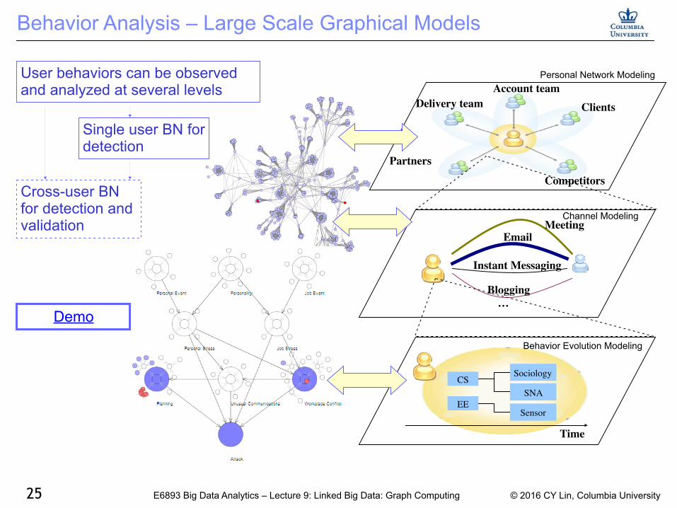
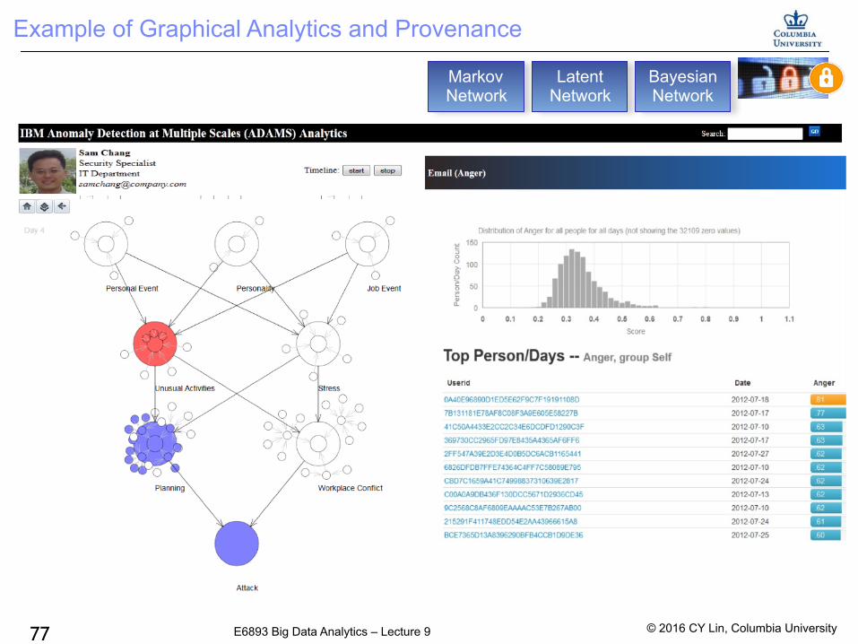
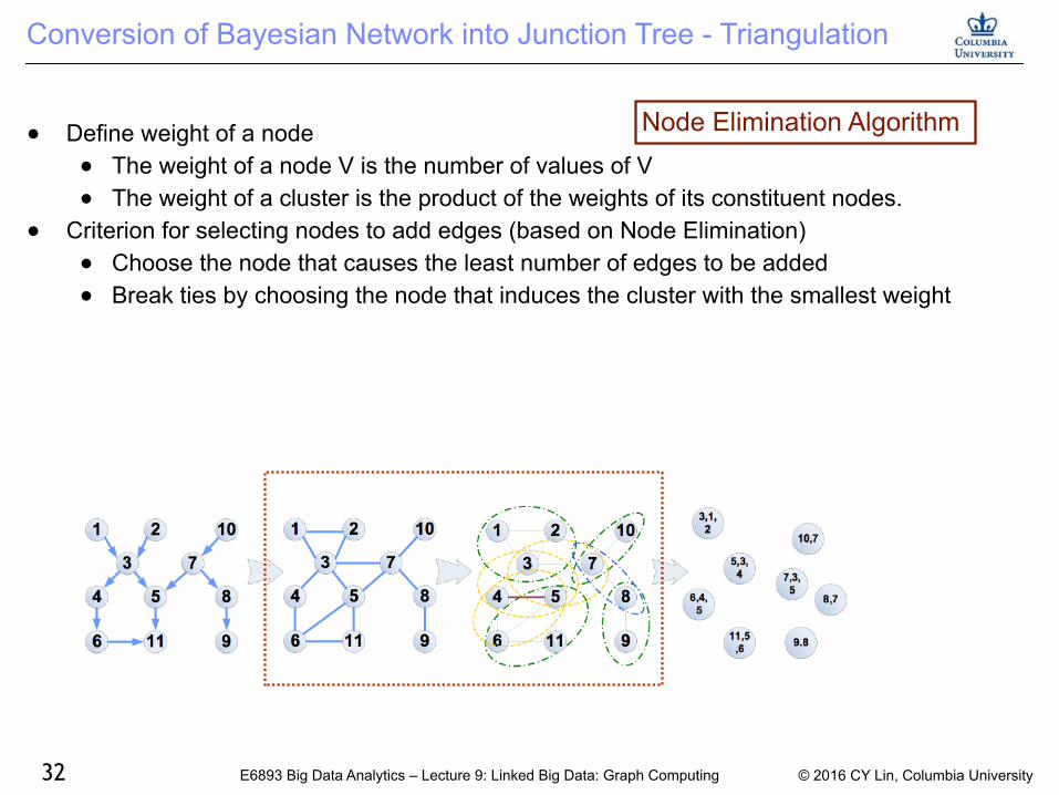
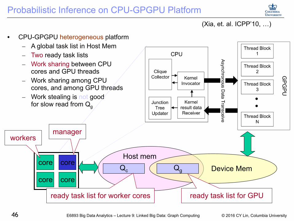
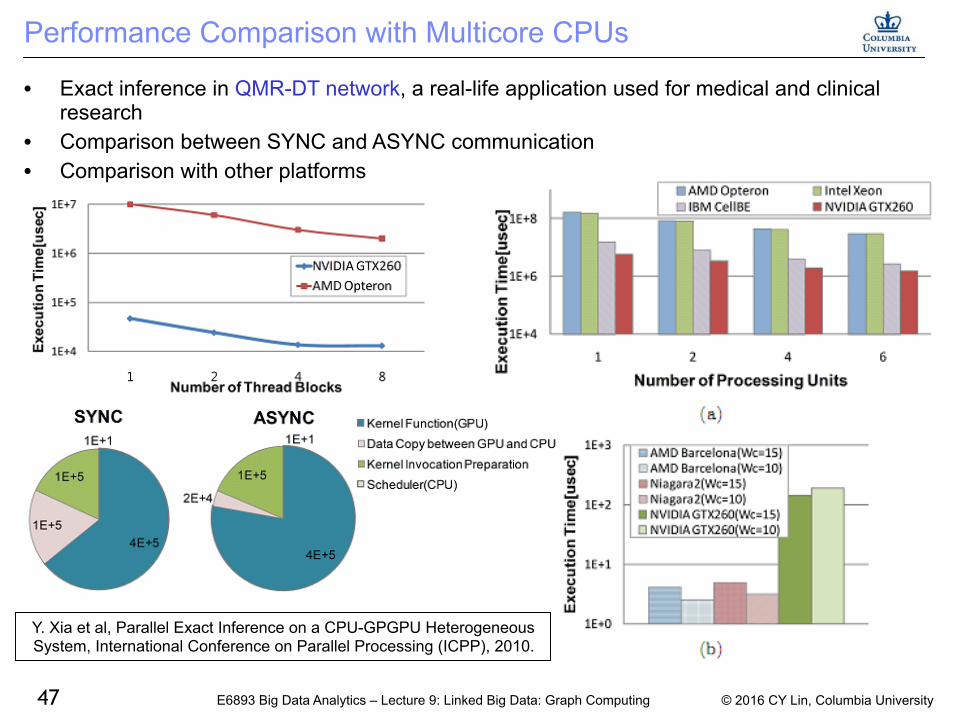
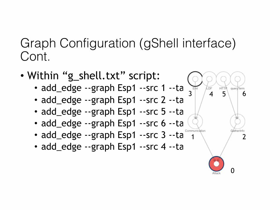

copy 2016 CY Lin Columbia UniversityE6893 Big Data Analytics ndash Lecture 9 Linked Big Data Graph Computing58
Demo by Eric Johnson


