
EC230B: Graduate Public Economics
Introduction and Road Map
Hilary Hoynes
1

EC230B
• Contacting me: [email protected]
• Course web site = bCourses.berkeley.edu
• Office hours Tuesday 3-5, sign up on wejoinin
• My office hours are in my office in the Goldman School,
Rm 345.
• Reed Walker is teaching the second half of the course (7
lectures each)
2

Thanks to others
The slides I am using this term are the result of a collaborationacross lots of other faculty teaching PE including:
Emmanuel and Gabriel
Raj Chetty
Day Manoli
John Friedman
Nathan Hendren
Owen Zidar
Amy Finkelstein
3

PUBLIC ECONOMICS DEFINITION
Public economics = Study of the role of the government in
the economy
Government is instrumental in most aspects of economic life:
1) Regulation: min wages, FDA regulations (25% of products consumed),zoning, labor laws, min education laws, environment
2) Taxes: governments in advanced economies collect 30-50% of NationalIncome in taxes
3) Expenditures: tax revenue funds traditional public goods (infrastruc-ture, public order and safety, defense), and welfare state (education,retirement benefits, health care, income support)
4) Macro-economic stabilization through central bank (interest rate, infla-tion control), fiscal stimulus, bailout policies
4

20%
30%
40%
50%
60%
Tota
l tax
reve
nues
(% n
atio
nal i
ncom
e)
Figure 13.1. Tax revenues in rich countries, 1870-2010
Sweden
France
U.K.
U.S.,
0%
10%
1870 1890 1910 1930 1950 1970 1990 2010
Tota
l tax
reve
nues
(% n
atio
nal i
ncom
e)
Total tax revenues were less than 10% of national income in rich countries until 1900-1910; they represent between 30% and 55% of national income in 2000-2010. Sources and series: see piketty.pse.ens.fr/capital21c.
Source: Piketty (2014)

Economic Arguments for Government Intervention
When is government intervention necessary in a market econ-
omy?
1) Failure of 1st Welfare Theorem: Government intervention
can help if there are market or individual failures
2) Building off 2nd Welfare Theorem: Distortionary Govern-
ment intervention is required to reduce economic inequality
6

Role 1: 1st Welfare Theorem Failure
1st Welfare Theorem: If (1) no externalities, (2) perfect
competition, (3) perfect information, (4) agents are rational,
then private market equilibrium is Pareto efficient
Government intervention may be desirable if:
1) Externalities require government interventions (Pigouvian taxes/subsidies,public good provision)
2) Imperfect competition requires regulation (typically studied in IndustrialOrganization)
3) Imperfect or Asymmetric Information (e.g., adverse selection may callfor mandatory insurance)
4) Agents are not rational (= individual not market failures analyzed inbehavioral economics, field in huge expansion): e.g., myopic or hyperbolicagents may not save enough for retirement
7

Role 2: 2nd Welfare Theorem Fallacy
Even with no market failures, free market might generate sub-stantial inequality. Inequality is an issue because of peoplecare about their relative situation.
2nd Welfare Theorem: Any Pareto Efficient outcome canbe reached by (1) Suitable redistribution of initial endowments[individualized lump-sum taxes based on indiv. characteristicsand not behavior], (2) Then letting markets work freely
⇒ No conflict between efficiency and equity [1st best taxation]
Redistribution of initial endowments is not feasible (informa-tion pb)⇒ govt needs to use distortionary taxes and transfers⇒ Trade-off between efficiency and equity [2nd best taxation]
This class will focus primarily on role 2
8

First Role for Government: Improve Efficiency
Public Economics Lectures Introduction 40 / 53

Second Role for Government: Improve Distribution
Public Economics Lectures Introduction 41 / 53
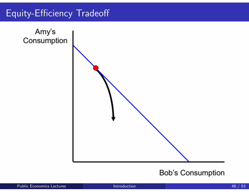
Equity-Efficiency Tradeoff
Public Economics Lectures Introduction 48 / 53

Normative vs. Positive Public Economics
Normative Public Economics: Analysis of How Things Shouldbe (e.g., should the government intervene in health insurancemarket? how high should taxes be?, etc.)
Positive Public Economics: Analysis of How Things ReallyAre; what are the effects of government programs and poli-cies? (e.g., Does govt provided health care crowd out privatehealth care insurance? Do higher taxes reduce labor supply?)
Positive Public Economics is a required 1st step before we cancomplete Normative Public Economics
Positive analysis is primarily empirical and Normative analysisis primarily theoretical
Positive Public Economics overlaps with Labor Economics
Political Economy is a positive analysis of govt outcomes
11

Plan for 230B Lectures
1) Labor Income Taxation and Redistribution (HOYNES):
(a) Labor Supply and Taxes, (b) Cash welfare, importance of
program take-up, (c) In-Kind transfers, (d) Public Health In-
surance, and (e) long run effects of the social safety net.
2) Environment meets public (WALKER)
See slides by Saez Normative Aspects: Optimal Income
Taxes and Transfers See slides by Zucman Wealth inequality
and taxing capital income
12

TODAY’S LECTURE
1. Labor market fundamentals
2. Measuring inequality; trends in inequality
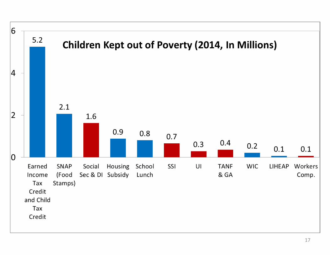
3. Measuring poverty, trends in poverty
4. Measuring Intergenerational inequality; trends in intergeninequality
5. Definitions in public economics; what does the govt do?
6. Opportunities: growth of RCTs, big data
13

1. Labor Market: Wages, Earnings, Employment
• Why do we start here?
• Trends in real earnings (at the lower end) and top tail
earnings are the most important component of poverty
and inequality
• EX: Stagnating or falling wages put upward pressure on
poverty
14

Autor, Science.
Trends by education level (Autor)

EPI, State of Working America.
Trends in percentiles of real wages
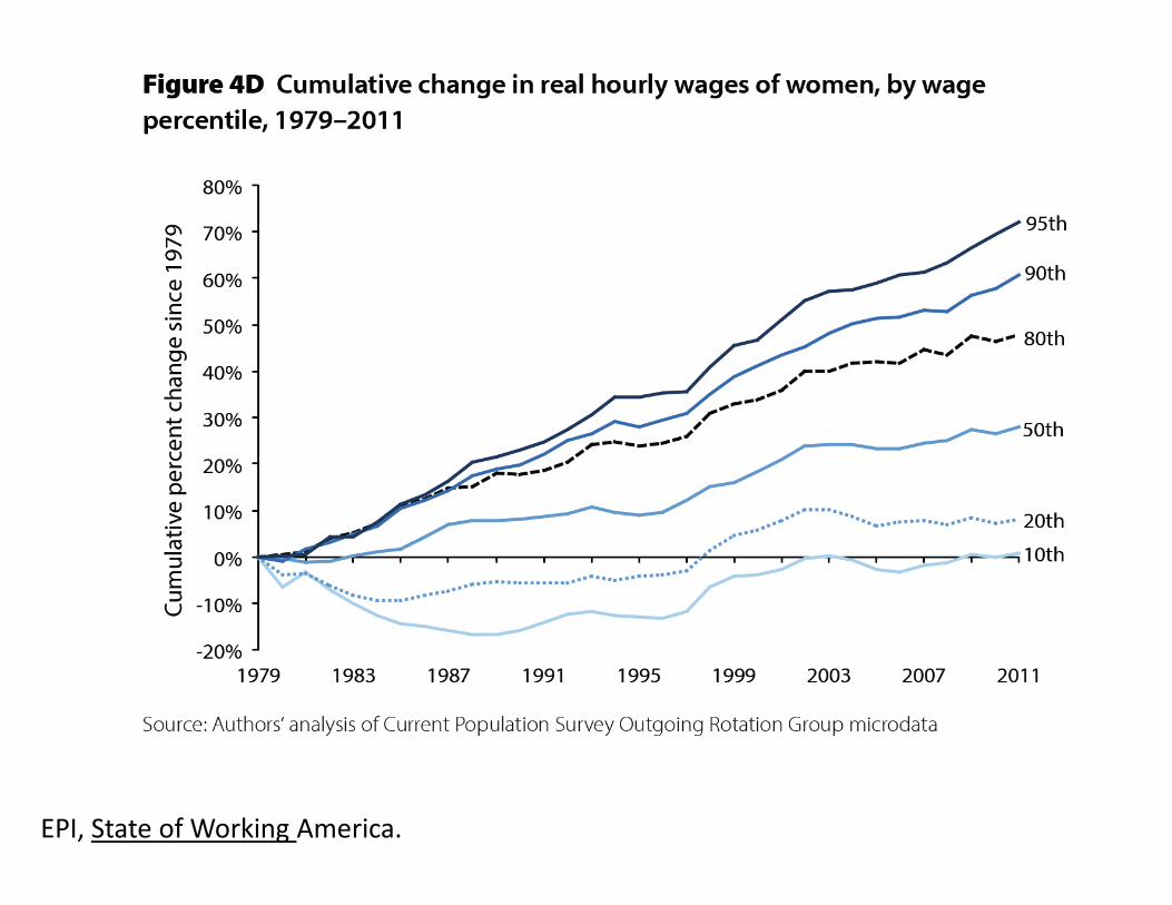
EPI, State of Working America.
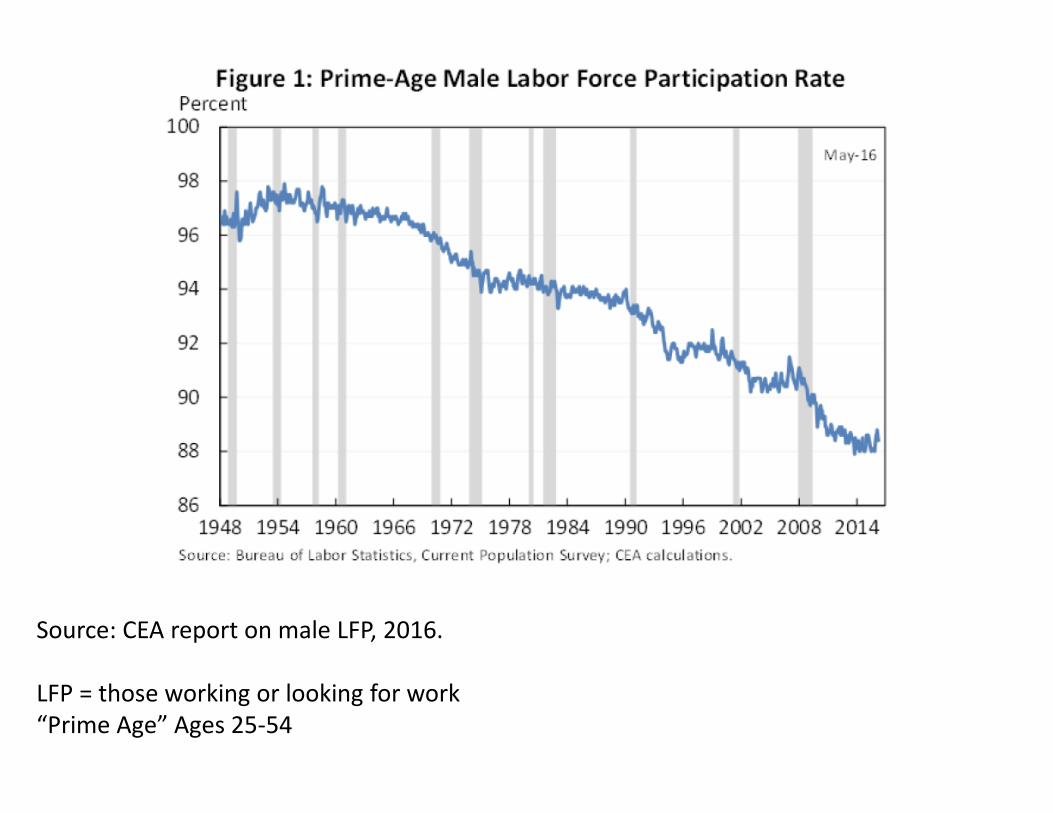
Source: CEA report on male LFP, 2016.
LFP = those working or looking for work“Prime Age” Ages 25-54
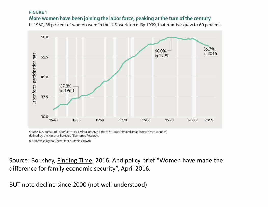
Source: Boushey, Finding Time, 2016. And policy brief “Women have made the difference for family economic security”, April 2016.
BUT note decline since 2000 (not well understood)

Economic Report of the President, 2015.
LFPR falling in US for men and women

Source: CEA report on male LFP, 2016.

Labor Market: Wages, Earnings, Employment (cont)
• If you put together declines in earnings and declines in
labor force participation, this is a powerful force in trends
in real household income
• Post WWII to early 1970s: gains in earnings occurred
across the distribution; growing together
• Mid 1970s to present: widening wage structure, growing
apart
We will see the data on this later.
16

2. INCOME INEQUALITY MEASUREMENT
Income Inequality: Labor vs. Capital Income
Individuals derive market income (before tax) from labor and
capital: z = wl + rk where w is wage, l is labor supply, k is
wealth, r is rate of return on wealth
1) Labor income inequality is due to differences in working
abilities (education, talent, physical ability, etc.), work effort
(hours of work, effort on the job, etc.), and luck (labor effort
might succeed or not)
2) Capital income inequality is due to differences in wealth
k (due to past saving behavior and inheritances received), and
in rates of return r (varies dramatically overtime and across
assets)
17
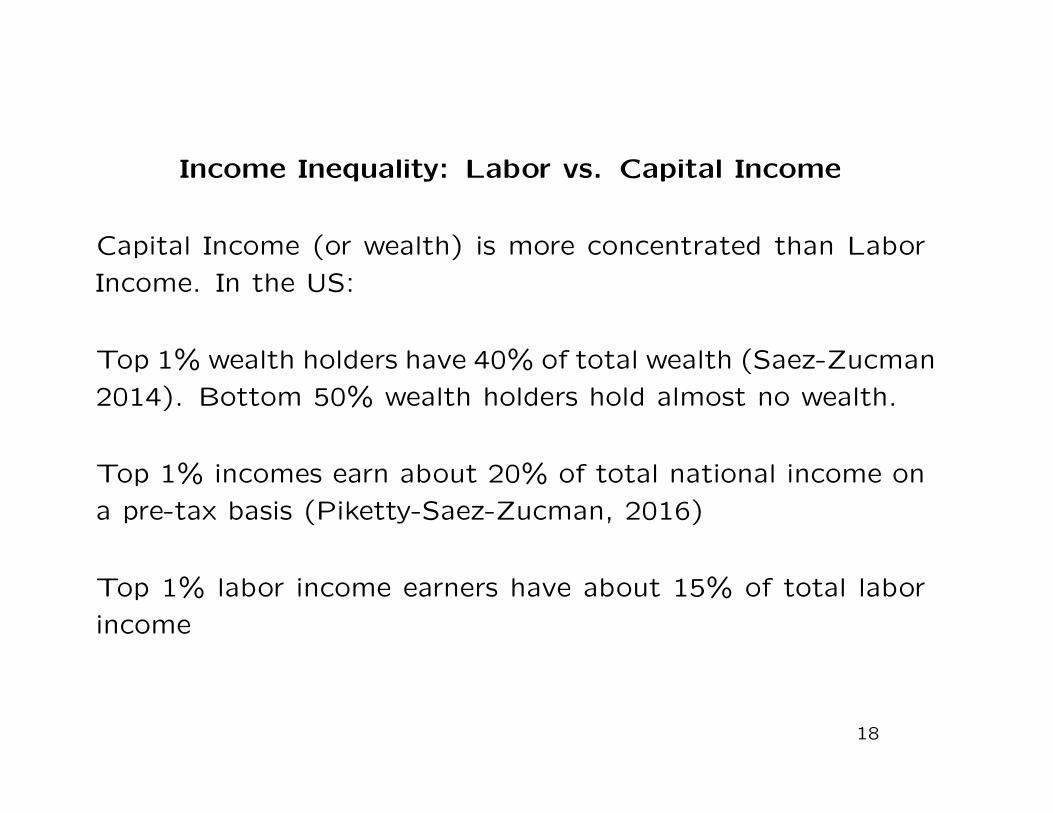
Income Inequality: Labor vs. Capital Income
Capital Income (or wealth) is more concentrated than Labor
Income. In the US:
Top 1% wealth holders have 40% of total wealth (Saez-Zucman
2014). Bottom 50% wealth holders hold almost no wealth.
Top 1% incomes earn about 20% of total national income on
a pre-tax basis (Piketty-Saez-Zucman, 2016)
Top 1% labor income earners have about 15% of total labor
income
18
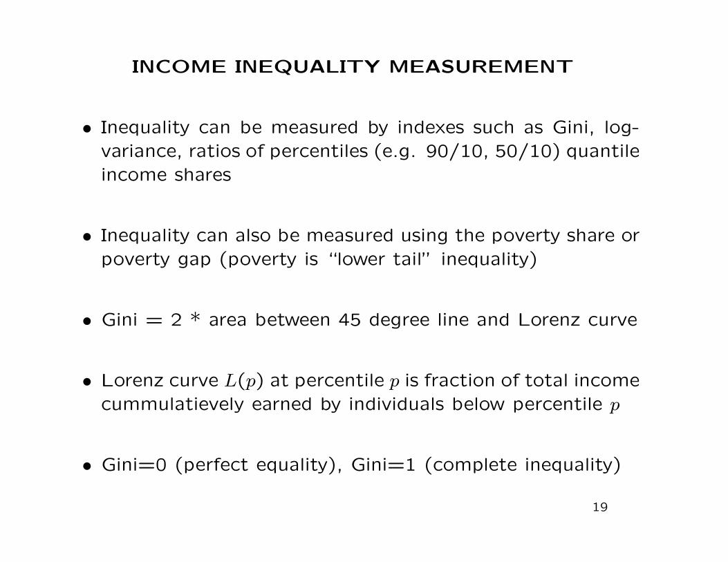
INCOME INEQUALITY MEASUREMENT
• Inequality can be measured by indexes such as Gini, log-variance, ratios of percentiles (e.g. 90/10, 50/10) quantileincome shares
• Inequality can also be measured using the poverty share orpoverty gap (poverty is “lower tail” inequality)
• Gini = 2 * area between 45 degree line and Lorenz curve
• Lorenz curve L(p) at percentile p is fraction of total incomecummulatievely earned by individuals below percentile p
• Gini=0 (perfect equality), Gini=1 (complete inequality)
19

Gini Coefficient California pre-tax income, 2000, Gini=62.1%
0%
10%
20%
30%
40%
50%
60%
70%
80%
90%
100%
0% 10% 20% 30% 40% 50% 60% 70% 80% 90% 100%
Lorenz Curve
45 degree line
Source: Annual Report 2001 California Franchise Tax Board

INCOME INEQUALITY MEASUREMENT (cont)
• Advantage of the Gini: one number, nice scaling
• Disadvantage of the Gini: not nuanced, does not tell you
about where inequality is
21

Top Income Shares: Piketty and Saez QJE-2003
• Getting data to measure the level and trend in incomes at the verytop of the distribution is hard. Standard survey data does not haveenough observations for these high income earners. And, surveysusually topcode income to protect anonymity
• Piketty and Saez came up with the novel idea of using data fromincome tax returns to estimate trends in top incomes. This is highquality data that is provided by most countries.
• These data are not well suited to measuring incomes at the lower tailof the distribution since many low income folks do not have to filetaxes. But it is exceedingly good data for measuring high income.
• Expanded to many countries (World Income Database, World Inequal-ity Report) Alvaredo-Chancel-Piketty-Saez-Zucman
22

Survey vs Admin Data for measuring inequality
• PLUS: Higher quality information: virtually no missing
data or attrition (CPS 30% nonresponse rate, underre-
porting of transfers getting worse over time)
• PLUS: Universe admin files mean ability to learn about
top incomes, can use rich nonparametric measures to learn
more
• NEG: only includes taxable income (misses transfers), non-
filer population is not small, not good for lower end of the
distribution
23

Key Empirical Facts on Income/Wealth Inequality
1) In the US, labor income inequality has increased substan-
tially since 1970: due to skilled biased technological progress
and institutions (min wage and Unions) [Autor-Katz’99]
2) US top income shares dropped dramatically from 1929 to
1950 and increased dramatically since 1980. Bottom 50%
incomes have stagnated in real terms since 1980 [Piketty-Saez-
Zucman ’16 distribute full National Income]
3) Fall in top income shares from 1900-1950 happened in
most OECD countries. Surge in top income shares has hap-
pened primarily in English speaking countries, and not as much
in Continental Europe and Japan [Atkinson, Piketty, Saez
JEL’11]
24

1940 1950 1960 1970 1980 1990 20000.30
0.35
0.40
0.45
0.50
Year
Gin
i coe
ffici
ent
● All WorkersMenWomen
●
●
● ● ●●
●
●● ●
●
●●
●●
●●
●● ●
●●
● ●● ● ● ● ●
● ● ●● ● ●
● ●●
● ●● ●
●
● ●
●●
● ●●
●
● ● ● ●
● ●●
●●
● ●●
●●
●●
●
●
●
● ● ●●
●
●● ●
●
●●
●●
●●
●● ●
●●
● ●● ● ● ● ●
● ● ●● ● ●
● ●●
● ●● ●
●
● ●
●●
● ●●
●
● ● ● ●
● ●●
●●
● ●●
●●
●●
●
Figure 1: Gini coefficient
Source: Kopczuk, Saez, Song QJE'10: Wage earnings inequality

Piketty & Saez, Science. Europe includes UK, France, Germany and Sweden.


• The period through the 1970s was similar in the U.S. compared to other countries suggesting that global factors were responsible
• The upward trend beginning in the late 1970s IS NOT experienced by all countries suggesting that global factors CAN NOT explain the trend

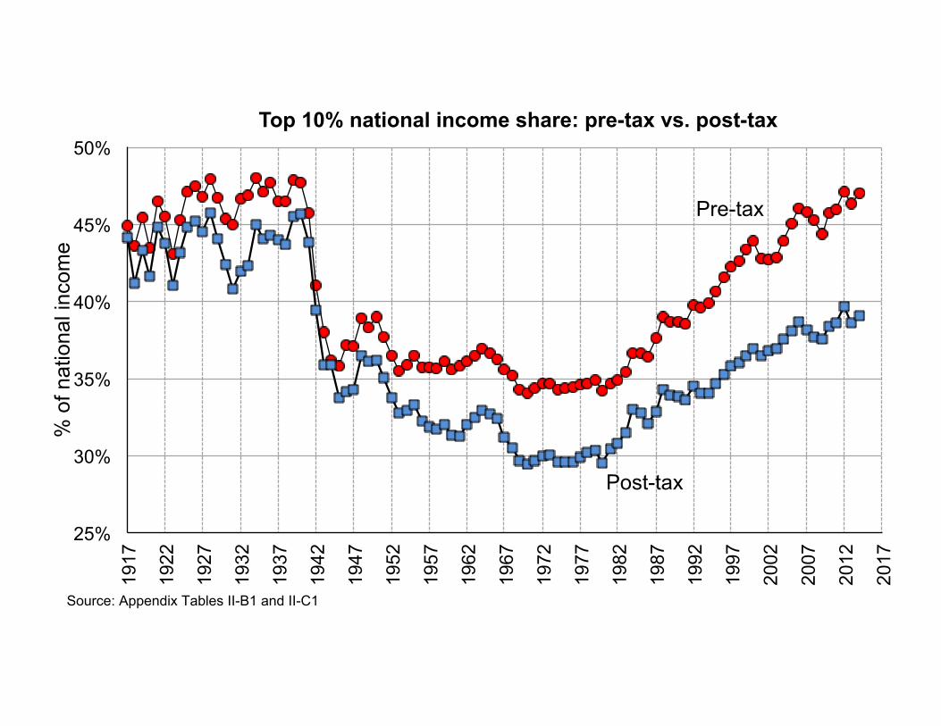
US Distributional Natl Accounts Piketty-Saez-Zucman
QJE-forth
• Expand beyond tax data to incorporate nonfilers and nontaxable in-come;
• combine tax, survey, and national accounts data to build new serieson the distribution of national income since 1913
• Use CPS to add nonfilers, also to allocate nontaxable income (govttransfers), also public goods
• Pre-tax income is income before taxes and transfers
• Post-tax income is income net of all taxes and adding all transfers andpublic good spending
27
25%
30%
35%
40%
45%
50% 19
17
1922
1927
1932
1937
1942
1947
1952
1957
1962
1967
1972
1977
1982
1987
1992
1997
2002
2007
2012
2017
% o
f nat
iona
l inc
ome
Top 10% national income share: pre-tax vs. post-tax
Pre-tax
Post-tax
Source: Appendix Tables II-B1 and II-C1

Piketty, Saez & Zucman, QJE forthcoming

Piketty, Saez & Zucman, QJE forthcoming

10%
12%
14%
16%
18%
20%
22% 19
62
1966
1970
1974
1978
1982
1986
1990
1994
1998
2002
2006
2010
2014
% o
f nat
iona
l inc
ome
Top 1% and Bottom 50% Adults pre-tax national income shares
Bottom 50%
Top 1%

3. Measuring Poverty
1. Define a threshold (equivalence scales used for varying
family sizes)
2. Define the resource measure
3. Define the economic sharing unit (typically family based
measure)
Then poor if resources < threshold
31

Alternative ways to measuring poverty
• Absolute vs Relative - e.g. OECD poverty is if below 50%
median income
• Consumption vs income
• Material deprivation (often used in developing country con-
text)
32

US poverty measurement
• Official poverty uses pre-tax cash income as resource
measure; threshold based on 1960 standard of 3 * cost
of food (orshansky measure); absolute measure
• Supplemental poverty measure introduced in 2011: re-
source measure is post-tax and includes inkind transfers;
threshold updated and varies across states (cost of hous-
ing)
• For SPM need to create consistent time series: Anchored
SPM (move thresholds back using CPI) and Historical SPM
(use available data to best mimic SPM threshold in earlier
years)
33


Why differential changes across age groups?
14

EROP 2014, Ch 6.
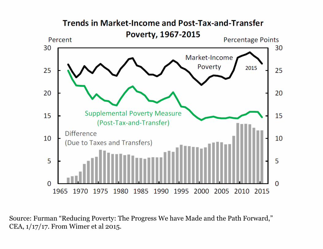
Source: Furman “Reducing Poverty: The Progress We have Made and the Path Forward,” CEA, 1/17/17. From Wimer et al 2015.
17

4. Measuring Intergenerational Income Mobility
Strong consensus that children’s success should not depend
too much on parental income [Equality of Opportunity]
Studies linking adult children to their parents can measure link
between children and parents income
Historically, standard measure was the correlation between fa-
thers and sons incomes or earnings, usually at some standard-
ized age (ingen elas IGE in log-log regression)
As with Gini, this gives us a good summary number, but it does
not tell us much about how this varies across the distribution
Historically, studies used survey data (limited granularity across
space and the income distribution)
35

Intergenerational Income Mobility
CHKS-QJE14 CHKS-AERPP14
The measure: average income rank of children by income rank
of parents (relative and absolute measure)
The data: Universe of tax filers, 1996-present, 1040 form plus
information returns (W-2)
The sample: Children, US citizens 1980-82 birth cohorts
Geography: Commuting zones (agg of counties, 741 CZs in
US, ave pop 380K)
36
Findings CHKS-QJE14 CHKS-AERPP14
1) US has less mobility than European countries (especially
Scandinavian countries such as Denmark)
2) Substantial heterogeneity in mobility across cities in the US
3) Places with low race/income segregation, low income in-
equality, good K-12 schools, high social capital, high family
stability tend to have high mobility [these are correlations and
do not imply causality]
4) has not changed very much over time (though their period
is short)
37
20
30
40
50
60
70
0 10 20 30 40 50 60 70 80 90 100
Me
an
Child
In
com
e R
an
k
Parent Income Rank
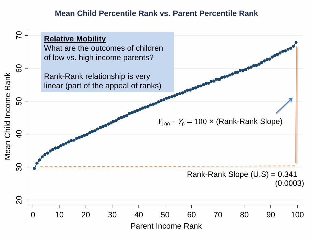
Mean Child Percentile Rank vs. Parent Percentile Rank
Rank-Rank Slope (U.S) = 0.341(0.0003)
Relative Mobility
What are the outcomes of children
of low vs. high income parents?
Rank-Rank relationship is very
linear (part of the appeal of ranks)
Y100 – Y0 = 100 × (Rank-Rank Slope)
20
30
40
50
60
70
0 10 20 30 40 50 60 70 80 90 100
Me
an
Child
In
com
e R
an
k
Parent Income Rank
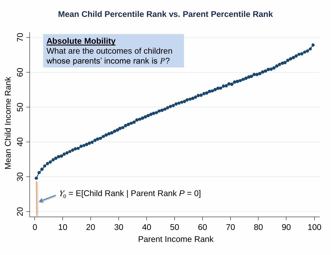
Mean Child Percentile Rank vs. Parent Percentile Rank
Absolute Mobility
What are the outcomes of children
whose parents’ income rank is 𝑃?
Y0 = E[Child Rank | Parent Rank P = 0]

20
30
40
50
60
70
0 10 20 30 40 50 60 70 80 90 100
Me
an
Child
In
com
e R
an
k
Parent Income Rank
Mean Child Percentile Rank vs. Parent Percentile Rank
Rank-Rank Slope (U.S) = 0.341(0.0003)
Run this regression, the two
parameters can get you rel and abs
mobility:
Rel mobility = 100 x b
Abs upward mobility (25th p) = a +
25 x b
𝑅𝑎𝑛𝑘𝑐ℎ𝑖𝑙𝑑 = 𝛼 + 𝛽𝑅𝑎𝑛𝑘𝑝𝑎𝑟𝑒𝑛𝑡 + 𝜀
𝑅𝑒𝑙𝑎𝑡𝑖𝑣𝑒 𝑀𝑜𝑏𝑖𝑙𝑖𝑡𝑦 = 100 x 𝛽

The Geography of Upward Mobility in the United States
Mean Child Percentile Rank for Parents at 25th Percentile (Y25)
Note: Lighter Color = More Absolute Upward Mobility

Upward MobilityCZ Name Y25 Y100 – Y0
P(Child in Q5|
Rank Parent in Q1)
1 Salt Lake City, UT 46.2 0.264 10.83%
2 Pittsburgh, PA 45.2 0.359 9.51%
3 San Jose, CA 44.7 0.235 12.93%
4 Boston, MA 44.6 0.322 10.49%
5 San Francisco, CA 44.4 0.250 12.15%
6 San Diego, CA 44.3 0.237 10.44%
7 Manchester, NH 44.2 0.296 10.02%
8 Minneapolis, MN 44.2 0.338 8.52%
9 Newark, NJ 44.1 0.350 10.24%
10 New York, NY 43.8 0.330 10.50%
Highest Absolute Mobility In The 50 Largest CZs
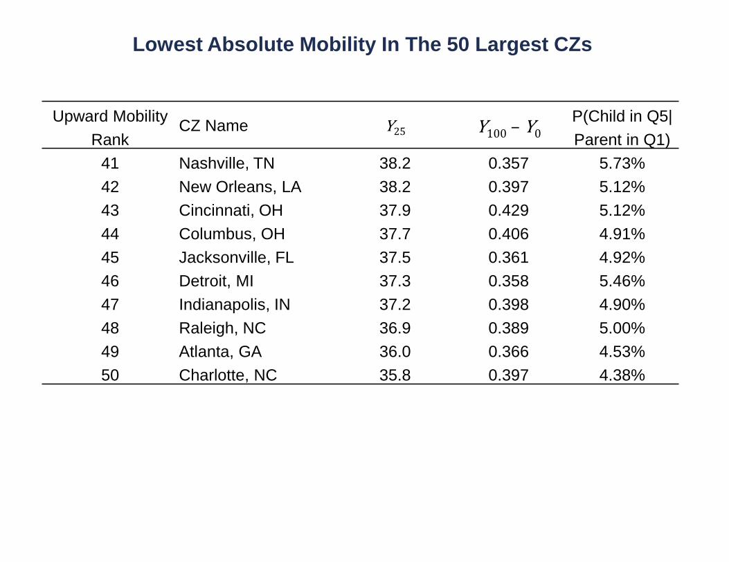
Upward MobilityCZ Name Y25 Y100 – Y0
P(Child in Q5|
Rank Parent in Q1)
41 Nashville, TN 38.2 0.357 5.73%
42 New Orleans, LA 38.2 0.397 5.12%
43 Cincinnati, OH 37.9 0.429 5.12%
44 Columbus, OH 37.7 0.406 4.91%
45 Jacksonville, FL 37.5 0.361 4.92%
46 Detroit, MI 37.3 0.358 5.46%
47 Indianapolis, IN 37.2 0.398 4.90%
48 Raleigh, NC 36.9 0.389 5.00%
49 Atlanta, GA 36.0 0.366 4.53%
50 Charlotte, NC 35.8 0.397 4.38%
Lowest Absolute Mobility In The 50 Largest CZs

Salt Lake City Charlotte
20
30
40
50
60
70
0 20 40 60 80 100
Salt Lake City: Y100 – Y0 = 26.4
Charlotte: Y100 – Y0 = 39.7
Intergenerational Mobility in Salt Lake City vs. CharlotteC
hild
Ran
k in N
atio
na
l In
co
me D
istr
ibutio
n
Parent Rank in National Income Distribution

Frac. Married (+)Divorce Rate (-)
Frac. Single Moms (-)
Violent Crime Rate (-)Frac. Religious (+)
Social Capital Index (+)
Share Foreign Born (-)Migration Outflow (-)
Migration Inflow (-)
Teenage LFP Rate (+)Chinese Import Growth (-)
Manufacturing Share (-)
Coll Grad Rate (Inc Adjusted) (+)College Tuition (-)
Colleges per Capita (+)
High School Dropout (-)Test Scores (Inc Adjusted) (+)
Student-Teacher Ratio (-)
Tax Progressivity (+)State EITC Exposure (+)
Local Tax Rate (+)
Top 1% Inc. Share (-)Gini Coef. (-)
Mean Household Income (+)
Frac. < 15 Mins to Work (+)Segregation of Poverty (-)
Racial Segregation (-)
0 0.2 0.4 0.6 0.8 1.0
TA
XC
OLL
MIG
SE
GFA
MS
OC
K-1
2IN
CL
AB
Spatial Correlates of Upward Mobility
Correlation

The Geography of Upward Mobility in the United States Odds of Reaching the Top Fifth Starting from the Bottom Fifth
SJ 12.9%
LA 9.6%
Atlanta 4.5%
Washington DC 11.0%
Charlotte 4.4%
Indianapolis 4.9%
Note: Lighter Color = More Upward Mobility Download Statistics for Your Area at www.equality-of-opportunity.org
SF 12.2%
San Diego 10.4%
SB 11.3%
Modesto 9.4% Sacramento 9.7%
Santa Rosa 10.0%
Fresno 7.5%
US average 7.5% [kids born 1980-2]
Bakersfield 12.2%
Source: Chetty et al. (2014)

FIGURE II: Association between Children’s Percentile Rank and Parents’ Percentile Rank
A. Mean Child Income Rank vs. Parent Income Rank in the U.S.
2030
4050
6070
0 10 20 30 40 50 60 70 80 90 100
Mea
n C
hild
Inco
me
Ran
k
Parent Income Rank
Rank-Rank Slope (U.S) = 0.341(0.0003)
B. United States vs. Denmark
2030
4050
6070
0 10 20 30 40 50 60 70 80 90 100
Mea
n C
hild
Inco
me
Ran
k
Parent Income Rank United StatesDenmark
Rank-Rank Slope (Denmark) = 0.180(0.0063)
Notes: These figures present non-parametric binned scatter plots of the relationship between child and parent income ranks.Both figures are based on the core sample (1980-82 birth cohorts) and baseline family income definitions for parents andchildren. Child income is the mean of 2011-2012 family income (when the child was around 30), while parent income is meanfamily income from 1996-2000. We define a child’s rank as her family income percentile rank relative to other children inher birth cohort and his parents’ rank as their family income percentile rank relative to other parents of children in the coresample. Panel A plots the mean child percentile rank within each parental percentile rank bin. The series in triangles in PanelB plots the analogous series for Denmark, computed by Boserup, Kopczuk, and Kreiner (2013) using a similar sample andincome definitions (see text for details). The series in circles reproduces the rank-rank relationship in the U.S. from Panel Aas a reference. The slopes and best-fit lines are estimated using an OLS regression on the micro data for the U.S. and on thebinned series (as we do not have access to the micro data) for Denmark. Standard errors are reported in parentheses.
Source: Chetty, Hendren, Kline, Saez (2014)

§ Probability that a child born to parents in the bottom fifth of the income distribution reaches the top fifth:
à Chances of achieving the “American Dream” are almost two times higher in Canada than in the U.S.
Canada
Denmark
UK
USA
13.5%
11.7%
7.5%
9.0% Blanden and Machin 2008
Boserup, Kopczuk, and Kreiner 2013
Corak and Heisz 1999
Chetty, Hendren, Kline, Saez 2014
The American Dream? Source: Chetty et al. (2014)

00
.20
.40
.60
.8
1971 1974 1977 1980 1983 1986 1989 1992Child's Birth Cohort
Intergenerational Mobility Estimates for the 1971-1993 Birth Cohorts
Income Rank-Rank
(Child Age 30; SOI Sample)
College-Income Gradient
(Child Age 19; Pop. Sample)Income Rank-Rank
(Child Age 26; Pop. Sample)
Ran
k-R
an
k S
lop
e Year by year regression and reporting of slope variable (child rank on parent rank).Very stable over time
1971-1982: uses smaller sample, universe of IRS data does not go back far enough.
1985+: too young for labor market outcomes, so use education instead

5. What does govt do? Taxes and Transfers
• Levels of govt: Fed, State, local
• Taxes, spending
• Spending: Social Insurance vs. Public Assistance, Cash
vs. In-Kind
• Funding: Entitlement (e.g. fully funded), Capped
42

Cash In Kind
Public Assistance (Means tested)
AFDC/TANFSSIGeneral AssistanceEITCChild Tax Credit (refundable)
SNAPWICSchool MealsMedicaidHousing programsLIHEAP
Social Insurance Social SecuritySSDIUnemployment InsWorkers Comp
Medicare

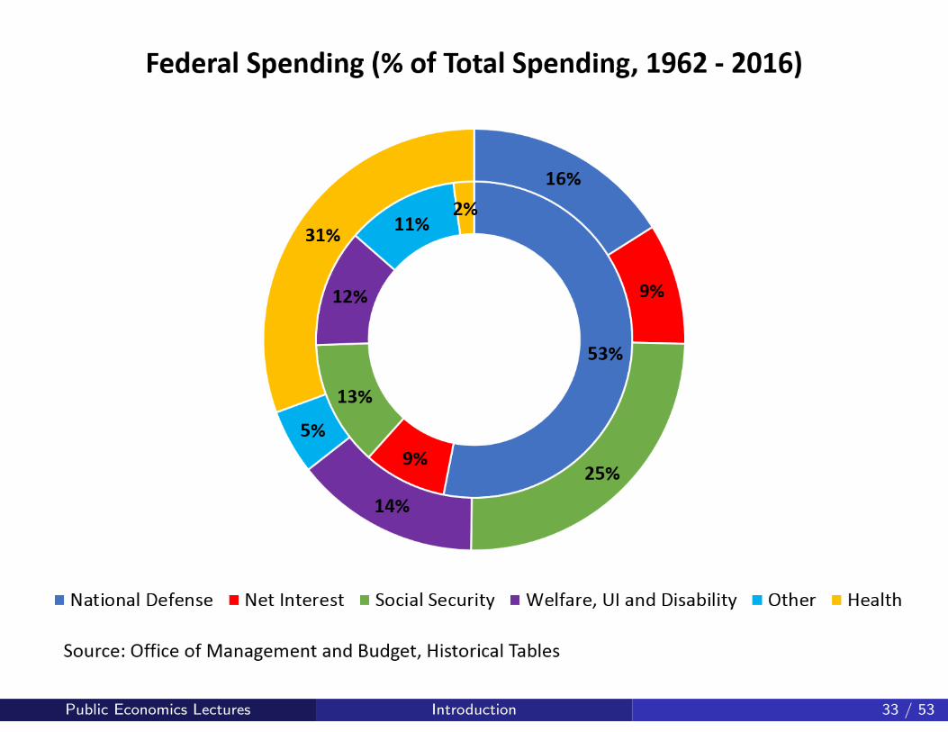
Background facts: Size and Comp of Govt
• Government expenditures = 1/3 GDP in the U.S.
• Higher than 50% of GDP in some European countries
• Decentralization is a key feature of U.S. govt
– Roughly 40% of spending (15% of GDP) is done at
state (e.g., food stamps) and local (e.g., schools) levels
item Rest (20% of GDP) is federal spending
• Tax expenditures” account for another 10% of GDP
44

Public Economics Lectures Introduction 30 / 53
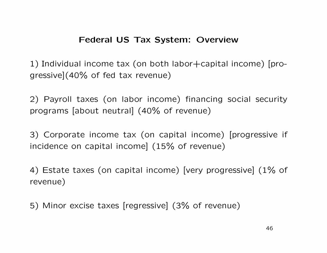
Federal US Tax System: Overview
1) Individual income tax (on both labor+capital income) [pro-
gressive](40% of fed tax revenue)
2) Payroll taxes (on labor income) financing social security
programs [about neutral] (40% of revenue)
3) Corporate income tax (on capital income) [progressive if
incidence on capital income] (15% of revenue)
4) Estate taxes (on capital income) [very progressive] (1% of
revenue)
5) Minor excise taxes [regressive] (3% of revenue)
46

State+Local Tax System: Overview
1) Individual+Corporate income taxes [progressive] (1/3 of
state+local tax revenue)
2) Sales + Excise taxes (tax on consumption = income -
savings) [about neutral] (1/3 of revenue)
3) Real estate property taxes (on capital income) [slightly pro-
gressive] (1/3 of revenue)
47

Public Economics Lectures Introduction 31 / 53

Public Economics Lectures Introduction 32 / 53
Public Economics Lectures Introduction 33 / 53


Tax and Transfer Benefits for Universally Available Programs (2015 $)
1992 policy 2015 policy
Source: Hoynes and Stabile (2017)

6. Opportunities: RCT, Admin Data
51

Admin Data
• Non-parametric, quasi-experimental methods (Event stud-ies, regression discontinuity, kink designs) require a lot ofdata
• Recent availability of very large datasets has transformedresearch in applied microeconomics
– Private: Scanner data on consumer purchases, healthinsurers, credit reports
– Public: Tax and social security records, school districtdatabases
• PE is data-driven, theoretically grounded approach to an-swering policy questions
52

1980 1990 2000 2010Year
Use of Pre-Existing Survey Data in Publications in Leading Journals, 1980-2010M
icro
-dat
a B
ased
Art
icle
s us
ing
Sur
vey
Dat
a (%
)
AER JPE QJE ECMA
Note: “Pre-existing survey” datasets refer to micro surveys such as the CPS or SIPP and do not include surveys designed by researchers for their study. Sample excludes studies whose primary data source is from developing countries.
100
80
60
40
20
0
Public Economics Lectures Introduction 15 / 53

Use of Administrative Data in Publications in Leading Journals, 1980-2010M
icro
-dat
a B
ased
Art
icle
s us
ing
Adm
in. D
ata
(%)
1980 1990 2000 2010Year
100
80
60
40
20
0
Note: “Administrative” datasets refer to any dataset that was collected without directly surveying individuals (e.g., scanner data, stock prices, school district records, social security records). Sample excludes studies whose primary data source is from developing countries.
AER JPE QJE ECMA
Public Economics Lectures Introduction 16 / 53

RCTs in Public Economics
• Growth beyond development economics
• Helped by JPAL North America
• Partner with state and local governments (Hastings and
Shapiro, RI SNAP and consumption)
• Partner with federal agencies (Bhargava and Manoli, IRS
EITC takeup)
54


