Download - ECE503: Digital Signal Processing Lecture 1

ECE503: Course Introduction
ECE503: Digital Signal ProcessingLecture 1
D. Richard Brown III
WPI
12-January-2012
WPI D. Richard Brown III 12-January-2012 1 / 56

ECE503: Course Introduction
Lecture 1 Major Topics
1. Administrative details: Course web page. Syllabus and textbook. Academic honesty policy. Students with disabilities statement.
2. Course Overview3. Notation
4. Mitra Chap 1: Signals and signal procesing5. Mitra Chap 2: Discrete-time signals in time domain6. Mitra Chap 3: Discrete-time signals in frequency
domain7. Bandpass sampling
8. Complex-valued signalsWPI D. Richard Brown III 12-January-2012 2 / 56

ECE503: Course Introduction
Signal Processing
“Roughly speaking, signal processing is concerned with the mathematicalrepresentation of the signal and the algorithmic operation carried out on itto extract the information present” (Mitra p. 1)
Lots of applications:
Audio signals
Communications
Biological signals (EMG, ECG, ...)
Radar/sonar
Image/video processing
Power metering
Structural health monitoring
... (see Mitra Chap. 1.4)
WPI D. Richard Brown III 12-January-2012 3 / 56
ECE503: Course Introduction
Digital Signal Processing
analog
input
sample
and hold
analog
to digital
converter
digital
processor
digital
to analog
converter
reconstruction
lter
analog
output
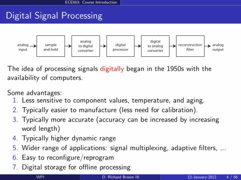
The idea of processing signals digitally began in the 1950s with theavailability of computers.
Some advantages:1. Less sensitive to component values, temperature, and aging.
2. Typically easier to manufacture (less need for calibration).
3. Typically more accurate (accuracy can be increased by increasingword length)
4. Typically higher dynamic range
5. Wider range of applications: signal multiplexing, adaptive filters, ...
6. Easy to reconfigure/reprogram
7. Digital storage for offline processingWPI D. Richard Brown III 12-January-2012 4 / 56

ECE503: Course Introduction
Digital Signal Processing
analog
input
sample
and hold
analog
to digital
converter
digital
processor
digital
to analog
converter
reconstruction
lter
analog
output
Some disadvantages:1. Increased system complexity
2. Potential for software bugs (more testing required)
3. Typically higher power consumption than analog circuits
4. Limited frequency range
5. Decreasing ADC/DAC accuracy as sampling frequency is increased
6. ADC and DAC delay
7. Finite precision effects
8. Analog circuits must be used for some applications (like what?)
WPI D. Richard Brown III 12-January-2012 5 / 56
ECE503: Course Introduction
Mitra Chapter 1
Signals and Signal Processing
1. Characterization and classification of signals Continuous-Time and Discrete-Time Continuous-Valued and Discrete-Valued Signal dimensionality
2. Typical Signal Processing Operations Scaling, delay, addition, product, integration, differentiation, filtering
(convolution), amplitude modulation, multiplexing, ...
3. Examples of typical signals
4. Typical signal processing applications
5. Why digital signal processing?
Please read 1-2 for review and skim 3-5 for context and motivation.
WPI D. Richard Brown III 12-January-2012 6 / 56

ECE503: Course Introduction
Some Notation
R = the set of real numbers (−∞,∞)
Z = the set of integers . . . ,−1, 0, 1, . . . j = unit imaginary number
√−1
C = the set of complex numbers (−∞,∞)× j(−∞,∞)
t = continuous time parameter ∈ R
x(t) = continuous-time signal R 7→ R or R 7→ C
n = discrete time parameter ∈ Z
x[n] = discrete-time signal Z 7→ R or Z 7→ C
T = sampling period ∈ R
FT = sampling frequency ∈ R
Ω = frequency of continuous-time signal ∈ R
ω = frequency of discrete-time signal ∈ R
WPI D. Richard Brown III 12-January-2012 7 / 56

ECE503: Course Introduction
Mitra Chapter 2
Discrete-Time Signals in the Time Domain1. Time-Domain Representation
Length and strength of a signal2. Operations on sequences
Scaling, delay, time-reversal, product, summation, filtering(convolution), sample rate conversion, ...
3. Operations on finite-length sequences Circular time-reversal, circular shifts
4. Classification of sequences Symmetry, periodicity, energy and power, bounded sequences,
absolutely summable sequences, square-summable sequences5. Typical sequences
Impulse (unit sample), unit step, sinusoidal, exponential, rectangularwindows, ...
Generating useful sequences in Matlab
6. The sampling process and aliasing
7. Correlation of signalsWPI D. Richard Brown III 12-January-2012 8 / 56

ECE503: Course Introduction
Representations of a Discrete-Time Signals
Example (Mitra sequence notation)
x[n] = 3,−3,1, 6↑
means x[−2] = 3, x[−1] = −3, x[0] = 1, and x[1] = 6.
We could also write this sequence as
x[n] = 3δ[n + 2]− 3δ[n + 1] + δ[n] + 6δ[n − 1]
where
δ[n] =
1 n = 0
0 otherwise
is the discrete-time unit impulse function.
If the sequence is given without an arrow, e.g. x[n] = 3,−3, 1, 6, it isimplied that the first element is at n = 0.
WPI D. Richard Brown III 12-January-2012 9 / 56
ECE503: Course Introduction
Length of a Discrete-Time Signal
Example:
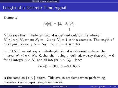
x[n] = 3,−3,1, 6↑
Mitra says this finite-length signal is defined only on the intervalN1 ≤ n ≤ N2 where N1 = −2 and N2 = 1 in this example. The length ofthis signal is clearly N = N2 −N1 + 1 = 4 samples.
In ECE503, we will say a finite-length signal is non-zero only on theinterval N1 ≤ n ≤ N2. Rather than being undefined, we say that x[n] = 0for all integer n < N1 and all integer n > N2. Hence
y[n] = 0, 0, 3,−3,1, 6, 0↑
is the same as x[n] above. This avoids problems when performingoperations on unequal length sequences.
WPI D. Richard Brown III 12-January-2012 10 / 56

ECE503: Course Introduction
Strength of a Discrete-Time Signal
The strength of a discrete-time signal is given by its norm. The Lp norm isdefined as
‖x‖p =
(∞∑
n=−∞
|x[n]|p)1/p
Typical values for p are p = 1, p = 2, and p = ∞.
Some facts:
‖x‖2/√N is the root-mean-squared (RMS) value of a length-N
sequence.
‖x‖22/N is the mean-squared value of a length-N sequence.
‖x‖1/N is the mean absolute value of a length-N sequence.
‖x‖2 ≤ ‖x‖1. ‖x‖∞ = maxn|x[n]|.
See the Matlab command norm.WPI D. Richard Brown III 12-January-2012 11 / 56

ECE503: Course Introduction
Discrete-Time Convolution
Assumes you understand the elementary operations of: Time shifting Time reversal Multiplication and addition
Given two sequences x[n] and h[n], we can convolve these sequencesto get a third sequence by computing
y[n] = x[n]⊛ h[n]
= h[n]⊛ x[n]
=∞∑
k=−∞
x[k]h[n − k]
=∞∑
k=−∞
h[k]x[n − k].
See the Matlab command conv and examples in Mitra Section 2.2.3.WPI D. Richard Brown III 12-January-2012 12 / 56

ECE503: Course Introduction
Sample-Rate Conversion (1 of 2)
Up-sampling by an integer factor L > 1:
xu[n] =
x[n/L] n = 0,±L,±2L, . . .
0 otherwise.
See Matlab command upsample.
Example: x[n] = 1, 2, 3 and L = 3.
−1 0 1 2 3 4 5 6 7 8 90
0.5
1
1.5
2
2.5
3
3.5
4
4.5
5
sample index
sam
ple
valu
e
WPI D. Richard Brown III 12-January-2012 13 / 56
ECE503: Course Introduction
Sample-Rate Conversion (2 of 2)
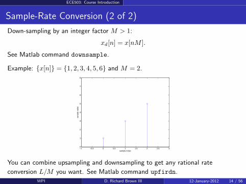
Down-sampling by an integer factor M > 1:
xd[n] = x[nM ].
See Matlab command downsample.
Example: x[n] = 1, 2, 3, 4, 5, 6 and M = 2.
−1 −0.5 0 0.5 1 1.5 2 2.5 30
1
2
3
4
5
6
7
8
sample index
sam
ple
valu
e
You can combine upsampling and downsampling to get any rational rate
conversion L/M you want. See Matlab command upfirdn.
WPI D. Richard Brown III 12-January-2012 14 / 56

ECE503: Course Introduction
Energy and Power Signals (1 of 2)
Total energy of the sequence x[n]:
Ex =∞∑
n=−∞
|x[n]|2 = ‖x‖22
Total energy is finite for all finite length sequences with finite valuedsamples and some infinite length sequences. A sequence that has finitetotal energy is called an energy signal.
For sequences that don’t have finite total energy, we can define theaverage power of an aperiodic sequence x[n] as:
Px = limK→∞
1
2K + 1
K∑
n=−K
|x[n]|2 (aperiodic sequences)
A sequence with non-zero finite average power is called a power signal.WPI D. Richard Brown III 12-January-2012 15 / 56

ECE503: Course Introduction
Energy and Power Signals (2 of 2)
For periodic sequences x[n] with period N , i.e. x[n+N ] = x[n] for alln, the average power is defined as
Px =1
N
n0+N−1∑
n=n0
|x[n]|2 (periodic sequences)
WPI D. Richard Brown III 12-January-2012 16 / 56

ECE503: Course Introduction
Sequence Boundedness and Summability
DefinitionA sequence x[n] is said to be bounded if there exists some finite Bx < ∞ such that
|x[n]| ≤ Bx for all n.
DefinitionA sequence x[n] is said to be absolutely summable if
∞∑
n=−∞
|x[n]| < ∞.
DefinitionA sequence x[n] is said to be square-summable if
∞∑
n=−∞
|x[n]|2 < ∞.
Such a sequence has finite energy and is an energy signal.
WPI D. Richard Brown III 12-January-2012 17 / 56

ECE503: Course Introduction
Typical Discrete-Time Sequences
Unit sample (discrete-time delta function):
δ[n] =
1 n = 0
0 otherwise
Unit step:
µ[n] =
1 n ≥ 0
0 otherwise
Note that δ[n] = µ[n]− µ[n− 1].
δ[n] is bounded, finite length, absolutely summable, and squaresummable.
µ[n] is bounded, infinite length (one-sided), not absolutely summable,and not square summable.
See Mitra pp. 64-67 for examples of sinusoidal and exponential sequences.WPI D. Richard Brown III 12-January-2012 18 / 56

ECE503: Course Introduction
Sequence Generation in Matlab
Some useful functions to generate discrete-time sequences in Matlab: exp sin cos square sawtooth
For example, to generate a half-second long exponentially decaying 100 Hzsinusoid sampled at FT = 800 Hz, one could write
Ttot = 0.5; % total time
OMEGA = 2*pi*100; % sinusoidal frequency
FT = 800; % sampling frequency (Hz)
T = 1/FT; % sampling period (sec)
n=0:Ttot*FT; % generate sampling indices
alpha = 1.5; % exponential decay factor
x = exp(-alpha*n*T).*sin(OMEGA*n*T);
stem(n,x); % plot sequence vs sample index
WPI D. Richard Brown III 12-January-2012 19 / 56

ECE503: Course Introduction
0 50 100 150 200 250 300 350 400−1
−0.8
−0.6
−0.4
−0.2
0
0.2
0.4
0.6
0.8
1
WPI D. Richard Brown III 12-January-2012 20 / 56

ECE503: Course Introduction
Normalized Frequency of Discrete-Time Signals
Ttot = 0.5; % total time
OMEGA = 2*pi*100; % sinusoidal frequency
FT = 800; % sampling frequency (Hz)
T = 1/FT; % sampling period (sec)
n=0:Ttot*FT; % generate sampling indices
alpha = 1.5; % exponential decay factor
x = exp(-alpha*n*T).*sin(OMEGA*n*T);
stem(n,x); % plot sequence vs sample index
Note the frequency of the continuous-time signal is Ω = 2π · 100radians/sec.
What is the frequency of the discrete-time signal? We specify thenormalized frequency of the discrete time signal in radians per sample as
ω = ΩT =Ω
FT
which implies that ω = 2π8 radians per sample in this example.
WPI D. Richard Brown III 12-January-2012 21 / 56

ECE503: Course Introduction
Non-Uniqueness of Discrete-Time Sinusoidal Signals
Suppose
x1[n] = sin(ωn+ φ)
x2[n] = sin((ω + k2π)n+ φ).
These two sequences are identical for any integer k ∈ Z.
This means there are an infinite number of continuous-time waveformsthat have the same discrete-time representation. In our previous example,suppose Ω = 2π · 900 radians per second. Then
ω =Ω
fT=
2π · 98
=2π
8+ 2π
Hence a 900 Hz sinusoidal signal looks exactly the same as a 100 Hz signalwhen they are sampled at FT = 800 Hz. This is an example of aliasing.
WPI D. Richard Brown III 12-January-2012 22 / 56

ECE503: Course Introduction
0 1 2 3 4 5 6 7 8−1
−0.8
−0.6
−0.4
−0.2
0
0.2
0.4
0.6
0.8
1
sample index
sam
ple
valu
e
WPI D. Richard Brown III 12-January-2012 23 / 56

ECE503: Course Introduction
Discrete-Time Correlation
Cross-correlation of two sequences x[n] and y[n]:
rxy[ℓ] =∞∑
n=−∞
x[n]y∗[n− ℓ] for ℓ ∈ Z
where ()∗ denotes complex conjugation (which has no effect if x[n] is areal-valued sequence). The parameter ℓ is called the “lag”.
1. Intuitively, a large correlation at lag ℓ indicates the sequence x[n] issimilar to the delayed sequence y[n− ℓ].
2. Intuitively, a small correlation at lag ℓ indicates the sequence x[n] notsimilar to the delayed sequence y[n− ℓ].
Autocorrelation of x[n] with itself:
rxx[ℓ] =
∞∑
n=−∞
x[n]x∗[n− ℓ] for ℓ ∈ Z
Note rxx[0] = Ex. See Mitra 2.6 for properties, normalized forms, what to do
with power and periodic signals, and how to compute correlations in Matlab.WPI D. Richard Brown III 12-January-2012 24 / 56

ECE503: Course Introduction
Discrete-Time Correlation Example
x = 0.98.^(abs(n-20))+0.1*randn(1,length(n));
y = 0.98.^(abs(n))+0.1*randn(1,length(n));
subplot(2,1,1)
plot(n,x,n,y);
grid on
xlabel(’sample index’);
ylabel(’signal values’);
subplot(2,1,2)
z = xcorr(x,y,100);
plot(n,z)
grid on
xlabel(’lag’);
ylabel(’correlation r_xy’);
WPI D. Richard Brown III 12-January-2012 25 / 56

ECE503: Course Introduction
−100 −80 −60 −40 −20 0 20 40 60 80 100−0.2
0
0.2
0.4
0.6
0.8
1
1.2
sample index
sign
al v
alue
s
−100 −80 −60 −40 −20 0 20 40 60 80 1000
10
20
30
40
50
lag
corr
elat
ion
r xy
WPI D. Richard Brown III 12-January-2012 26 / 56

ECE503: Course Introduction
Mitra Chapter 3
Discrete-Time Signals in the Frequency Domain
1. Continuous-Time Fourier Transform (CTFT) Definition and properties Parseval’s Theorem
2. Discrete-Time Fourier Transform (DTFT) Definition and properties Convergence conditions Relationship between DTFT and CTFT Parseval’s Theorem
3. Sampling Theorem
4. Bandpass Sampling
WPI D. Richard Brown III 12-January-2012 27 / 56

ECE503: Course Introduction
Continuous-Time Fourier Transform
X(Ω) =
∫∞
−∞
x(t)e−jΩt dt (CTFT)
x(t) =1
2π
∫∞
−∞
X(Ω)ejΩt dΩ (inverse CTFT)
Note x(t) is defined for all t ∈ R and X(Ω) is defined for all Ω ∈ R.
The spectrum X(Ω) is typically complex, even if x(t) is real. |X(Ω)| is called the “magnitude spectrum”. ∠X(Ω) is called the “phase spectrum”.
Sufficient conditions for the CTFT of x(t) to exist (Dirichlet conditions):
1. The signal x(t) has a finite number of finite discontinuities and afinite number of maxima and minima in any finite interval
2. The signal x(t) is absolutely integrable, i.e.∫
∞
−∞
|x(t)| dt < ∞
WPI D. Richard Brown III 12-January-2012 28 / 56

ECE503: Course Introduction
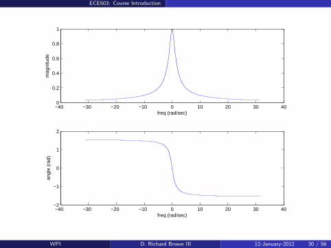
Continuous-Time Fourier Transform Example
Given x(t) = e−αtµ(t) with α > 0, we can directly confirm x(t) isabsolutely integrable and do the integration to compute
X(Ω) =1
α+ jΩ
Can compute magnitude and phase analytically (see Mitra example 3.1).We can also plot the magnitude and phase in Matlab:
alpha = 1;
OMEGA = 2*pi*[-5:0.01:5];
X = 1./(alpha+j*OMEGA);
subplot(2,1,1);
plot(OMEGA,abs(X));
xlabel(’freq (rad/sec)’);
ylabel(’magnitude’);
subplot(2,1,2)
plot(OMEGA,angle(X)); % may need unwrap(angle(X))
xlabel(’freq (rad/sec)’);
ylabel(’angle (rad)’);
WPI D. Richard Brown III 12-January-2012 29 / 56
ECE503: Course Introduction
−40 −30 −20 −10 0 10 20 30 400
0.2
0.4
0.6
0.8
1
freq (rad/sec)
mag
nitu
de
−40 −30 −20 −10 0 10 20 30 40−2
−1
0
1
2
freq (rad/sec)
angl
e (r
ad)
WPI D. Richard Brown III 12-January-2012 30 / 56

ECE503: Course Introduction
Parseval’s Theorem for Continuous-Time Signals
If a continuous-time signal x(t) has finite energy, then
Ex =
∫∞
−∞
|x(t)|2 dt = 1
2π
∫∞
−∞
|X(Ω)|2 dΩ < ∞
See the proof in your textbook. Units:
Ex is energy (joules).
|x(t)|2 is energy per second, which is power (watts).
|X(Ω)|2 is energy per unit frequency (joules/(rad/sec) orjoule-sec/rad).
Your textbook uses the notation Sxx(Ω) = |X(Ω)|2 to mean the “energydensity spectrum”. You can compute the amount of energy in a particularfrequency range a < Ω < b by computing
1
2π
∫ b
a|X(Ω)|2 dΩ
WPI D. Richard Brown III 12-January-2012 31 / 56

ECE503: Course Introduction
Poisson’s Sum Formula for Continuous-Time Signals
Given a continuous-time signal z(t) with CTFT Z(Ω), we can write theinfinite sum of delayed copies of z(t) as
z(t) =∞∑
n=−∞
z(t− nT ) =1
T
∞∑
n=−∞
Z(nΩT )ejnΩT t
where ΩT = 2π/T .
Proof sketch: Note that z(t) is periodic with period T and can berepresented as a Fourier series
z(t) =∞∑
n=−∞
αnejnΩT t
The Fourier series coefficients can be computed as αn = 1T Z(nΩT ).
WPI D. Richard Brown III 12-January-2012 32 / 56
ECE503: Course Introduction
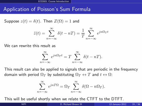
Application of Poisson’s Sum Formula
Suppose z(t) = δ(t). Then Z(Ω) = 1 and
z(t) =
∞∑
n=−∞
δ(t− nT ) =1
T
∞∑
n=−∞
ejnΩT t
We can rewrite this result as
∞∑
n=−∞
ejnΩT t = T∞∑
n=−∞
δ(t− nT ).
This result can also be applied to signals that are periodic in the frequencydomain with period ΩT by substituting ΩT ↔ T and t ↔ Ω:
∞∑
n=−∞
ejnTΩ = ΩT
∞∑
n=−∞
δ(Ω − nΩT ).
This will be useful shortly when we relate the CTFT to the DTFT.WPI D. Richard Brown III 12-January-2012 33 / 56

ECE503: Course Introduction
Discrete-Time Fourier Transform
X(ω) =∞∑
n=−∞
x[n]e−jωn (DTFT)
x[n] =1
2π
∫ π
−πX(ω)ejωn dω (inverse DTFT)
Note x[n] is defined for all n ∈ Z and X(ω) is defined for all ω ∈ R.
The spectrum X(ω) is typically complex, even if x[n] is real. |X(ω)| is called the “magnitude spectrum”. ∠X(ω) is called the “phase spectrum”.
Unlike the CTFT X(Ω), the DTFT X(ω) is periodic such thatX(ω + k2π) = X(ω) for any k ∈ Z. Easy to see from the definition:
X(ω + k2π) =
∞∑
n=−∞
x[n]e−j(ω+k2π)n =
∞∑
n=−∞
x[n]e−jωn e−jk2πn︸ ︷︷ ︸
=1
= X(ω)
WPI D. Richard Brown III 12-January-2012 34 / 56

ECE503: Course Introduction
Parseval’s Theorem for Discrete-Time Signals
If a discrete-time signal x[n] has finite energy, then
Ex =∞∑
n=−∞
|x[n]|2 = 1
2π
∫ π
−π|X(ω)|2 dω < ∞
See the proof in your textbook.
Your textbook uses the notation Sxx(ω) = |X(ω)|2 to mean the “energydensity spectrum”. You can compute the amount of energy in a particular(normalized) frequency range a < ω < b by computing
1
2π
∫ b
a|X(ω)|2 dω
WPI D. Richard Brown III 12-January-2012 35 / 56

ECE503: Course Introduction
Computation of the DTFT in Matlab
There are lots of ways to do this, but freqz is a good choice.
Typical usage:
N = 1001;
w = linspace(-pi,pi,N);
A = 1;
x = 0.95.^[0:100]; % example sequence
h = freqz(x,A,w);
subplot(2,1,1);
plot(w,abs(h));
xlabel(’normalized freq (rad/sample)’);
ylabel(’magnitude’);
subplot(2,1,2);
plot(w,unwrap(angle((h))));
xlabel(’normalized freq (rad/sample)’);
ylabel(’angle’);
WPI D. Richard Brown III 12-January-2012 36 / 56

ECE503: Course Introduction
−4 −3 −2 −1 0 1 2 3 40
5
10
15
20
normalized freq (rad/sample)
mag
nitu
de
−4 −3 −2 −1 0 1 2 3 4−1.5
−1
−0.5
0
0.5
1
1.5
normalized freq (rad/sample)
angl
e
WPI D. Richard Brown III 12-January-2012 37 / 56

ECE503: Course Introduction
Relationship Between the CTFT and the DTFT (1 of 4)
Ideal sampling and reconstruction process:
impulsegenerator
reconstruction lter
u(t)
p(t)
v(t) ∫ nT+ǫnT−ǫ dt
x[n] v(t)h(t) y(t)
The pulse train
p(t) =
∞∑
n=−∞
δ(t−nT ) ↔ P (Ω) =
∞∑
n=−∞
e−jΩnT = ΩT
∞∑
n=−∞
δ(Ω−nΩT )
causes
v(t) = u(t)p(t) =
∞∑
n=−∞
u(nT )δ(t− nT )
hence the discrete-time signal
x[n] =
∫ nT+ǫ
nT−ǫv(t) dt =
∫ nT+ǫ
nT−ǫ
∞∑
n=−∞
u(nT )δ(t− nT ) dt = u(nT ).
WPI D. Richard Brown III 12-January-2012 38 / 56
ECE503: Course Introduction
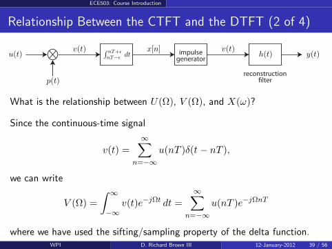
Relationship Between the CTFT and the DTFT (2 of 4)
impulsegenerator
reconstruction lter
u(t)
p(t)
v(t) ∫ nT+ǫnT−ǫ dt
x[n] v(t)h(t) y(t)
What is the relationship between U(Ω), V (Ω), and X(ω)?
Since the continuous-time signal
v(t) =
∞∑
n=−∞
u(nT )δ(t − nT ),
we can write
V (Ω) =
∫∞
−∞
v(t)e−jΩt dt =
∞∑
n=−∞
u(nT )e−jΩnT
where we have used the sifting/sampling property of the delta function.WPI D. Richard Brown III 12-January-2012 39 / 56

ECE503: Course Introduction
Relationship Between the CTFT and the DTFT (3 of 4)
We have
V (Ω) =
∞∑
n=−∞
u(nT )e−jΩnT .
We can develop a more direct expression relating V (Ω) and U(Ω) byrecalling v(t) = u(t)p(t) and using the multiplication property of theCTFT:
V (Ω) =1
2πU(Ω)⊛ P (Ω)
=1
2πU(Ω)⊛
(
ΩT
∞∑
n=−∞
δ(Ω − nΩT )
)
=1
T
∞∑
n=−∞
U(Ω− nΩT )
where ΩT = 2πFT = 2π/T is the sampling frequency in radians/sec.WPI D. Richard Brown III 12-January-2012 40 / 56

ECE503: Course Introduction
Relationship Between the CTFT and the DTFT (4 of 4)
We now have
V (Ω) =
∞∑
n=−∞
u(nT )e−jΩnT (1)
=1
T
∞∑
n=−∞
U(Ω− nΩT ). (2)
Recall the DTFT of x[n] = u(nT ) is
X(ω) =
∞∑
n=−∞
x[n]e−jωn =
∞∑
n=−∞
u(nT )e−jωn
Comparison with (1) reveals that X(ω) = V (Ω)|Ω=ω/T . Plugging this result into(2) gives the desired result:
X(ω) =1
T
∞∑
n=−∞
U(ω/T − n2π/T )
since ΩT = 2π/T .WPI D. Richard Brown III 12-January-2012 41 / 56

ECE503: Course Introduction
Sampling Theorem
impulsegenerator
reconstruction lter
u(t)
p(t)
v(t) ∫ nT+ǫnT−ǫ dt
x[n] v(t)h(t) y(t)
The impulse generator simply converts the discrete time sequence x[n]to the continuous time signal
v(t) =
∞∑
n=−∞
x[n]δ(t − nT ) =
∞∑
n=−∞
u(nT )δ(t− nT )
for which we previously derived the spectrum
V (Ω) =1
T
∞∑
n=−∞
U(Ω− nΩT ).
Under what conditions will y(t) = u(t)?WPI D. Richard Brown III 12-January-2012 42 / 56

ECE503: Course Introduction
Bandpass Sampling (1 of 5)
There are many signal processing situations, e.g. wireless communications,in which we would like to sample a bandpass signal, i.e. a signal withnon-zero spectrum only on 0 < a < |Ω| < b.
Ωa b−a−b
|U(Ω)|
We know we could satisfy the sampling theorem by just setting ΩT > 2b,but this is often impractical because the frequency b is often very large,e.g. 2.4 GHz.
Another approach is called bandpass sampling.
WPI D. Richard Brown III 12-January-2012 43 / 56

ECE503: Course Introduction
Bandpass Sampling (2 of 5)
Ωa b−a−b
|U(Ω)|
Example: Suppose a = 17.5 MHz and b = 22.5 MHz. We could justsample at FT = 45 MHz but this would require a fast sampler and lots offast memory to store and process the sampled signal.
What would happen if we sampled at FT = 17.5 MHz?
17.5 22.512.55-5-17.5-22.5 -12.5Ω
|V (Ω)|
Aliasing occurs but the replicated spectra do not overlap.WPI D. Richard Brown III 12-January-2012 44 / 56

ECE503: Course Introduction
Bandpass Sampling (3 of 5)
Can we have an even lower sampling rate and still avoid overlap?
Define the bandwidth and center frequency of the bandpass signal asB = b− a and Ωc = (b+ a)/2, respectively.
a b-a-b
P Q
Ω
−Ωc Ωc
2Ωc −B
We denote the number of spectral replicas between −Ωc and Ωc as m. Inthis example, we have m = 6.
The sampling frequency that achieves this spectral replication pattern is
ΩT1=
2Ωc −B
m.
WPI D. Richard Brown III 12-January-2012 45 / 56

ECE503: Course Introduction
Bandpass Sampling (4 of 5)
a b-a-b
P Q
Ω
−Ωc Ωc
2Ωc −B
The sampling frequency that achieves this spectral replication pattern is
ΩT1=
2Ωc −B
m.
If we increase the sampling frequency from this value, the replicas P andQ will overlap. So this means that, given a choice of m spectral replicas,
ΩT1≤ 2Ωc −B
m.
WPI D. Richard Brown III 12-January-2012 46 / 56

ECE503: Course Introduction
Bandpass Sampling (5 of 5)
If we decrease the sampling frequency from this value, the replicas P andQ will begin to separate and eventually abut R and S as shown below.
a b-a-b
P QR S
Ω
−Ωc Ωc
2Ωc −B
The sampling frequency that achieves this spectral replication pattern is
ΩT2=
2Ωc +B
m+ 1.
We do not want to decrease the sampling frequency below this point,otherwise we will have overlap. All of this implies
2Ωc +B
m+ 1≤ ΩT ≤ 2Ωc −B
m.
WPI D. Richard Brown III 12-January-2012 47 / 56
ECE503: Course Introduction
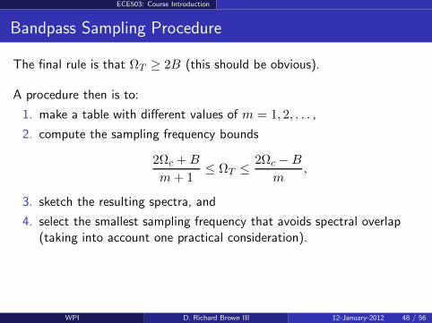
Bandpass Sampling Procedure
The final rule is that ΩT ≥ 2B (this should be obvious).
A procedure then is to:
1. make a table with different values of m = 1, 2, . . . ,
2. compute the sampling frequency bounds
2Ωc +B
m+ 1≤ ΩT ≤ 2Ωc −B
m,
3. sketch the resulting spectra, and
4. select the smallest sampling frequency that avoids spectral overlap(taking into account one practical consideration).
WPI D. Richard Brown III 12-January-2012 48 / 56
ECE503: Course Introduction
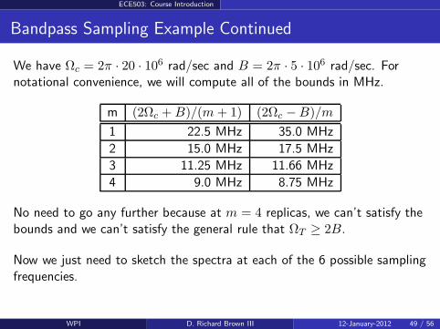
Bandpass Sampling Example Continued
We have Ωc = 2π · 20 · 106 rad/sec and B = 2π · 5 · 106 rad/sec. Fornotational convenience, we will compute all of the bounds in MHz.
m (2Ωc +B)/(m+ 1) (2Ωc −B)/m
1 22.5 MHz 35.0 MHz
2 15.0 MHz 17.5 MHz
3 11.25 MHz 11.66 MHz
4 9.0 MHz 8.75 MHz
No need to go any further because at m = 4 replicas, we can’t satisfy thebounds and we can’t satisfy the general rule that ΩT ≥ 2B.
Now we just need to sketch the spectra at each of the 6 possible samplingfrequencies.
WPI D. Richard Brown III 12-January-2012 49 / 56

ECE503: Course Introduction
20-20
FT = 22.5MHz
20-20
FT = 35MHz
20-20
FT = 15MHz
20-20
FT = 17.5MHz
20-20
FT = 11.25MHz
20-20
FT = 11.66MHz
ΩΩ
ΩΩ
ΩΩ
WPI D. Richard Brown III 12-January-2012 50 / 56

ECE503: Course Introduction
Bandpass Sampling: Some Practical Considerations
For odd values of m, note that the baseband spectrum is flipped withrespect to the original passband spectrum. This is called “spectralinversion”.
It doesn’t matter if the passband signals have symmetric spectra(around Ωc).
If you want to avoid it, make sure you pick an even value of m.
You can easily correct for spectral inversion after the fact bymultiplying the spectrally inverted sequence by (−1)n = cos(πn).
Broadband background noise can also cause problems in bandpasssampling unless filtered first.
WPI D. Richard Brown III 12-January-2012 51 / 56

ECE503: Course Introduction
What is a Complex Signal?
In the real world, all signals are real valued. A complex signal likex(t) = ejΩt can’t be generated. Or can it?
In many real-world applications like communication or radar systems, weoften work with two-dimensional real-valued signals that have a certainrelationship. It is often more convenient to represent these signals as asingle complex-valued signal (sometimes called a “quadrature signal”).
For example:
x1(t) = cos(Ωt)
x2(t) = sin(Ωt)
Both of these signals are real-valued. We can definex(t) = x1(t) + jx2(t) = ejΩt. This signal is complex-valued.
WPI D. Richard Brown III 12-January-2012 52 / 56

ECE503: Course Introduction
Complex Signal Notation Convenience (1 of 2)
Suppose you have four real-valued signals
x1(t) = cos(Ωt)
x2(t) = sin(Ωt)
y1(t) = cos(Ωt+ φ)
y2(t) = − sin(Ωt+ φ)
and have a real system (a “quadrature downconverter”) that computes
z1(t) = x1(t)y1(t)− x2(t)y2(t)
z2(t) = x1(t)y2(t) + x2(t)y1(t)
You can do all of the trigonometry to compute
z1(t) = cos(φ)
z2(t) = sin(−φ)
(continued...)WPI D. Richard Brown III 12-January-2012 53 / 56

ECE503: Course Introduction
Complex Signal Notation Convenience (2 of 2)
... or you could use complex notation:
x(t) = x1(t) + jx2(t) = ejΩt
y(t) = y1(t) + jy2(t) = e−j(Ωt+φ).
Recognizing that the quadrature downconverter is just performing complexmultiplication, we can write
z(t) = x(t)y(t)
= ejΩte−j(Ωt+φ)
= e−jφ
= cos(φ)− j sin(φ)
which is the same as saying
z1(t) = cos(φ)
z2(t) = sin(−φ).
WPI D. Richard Brown III 12-January-2012 54 / 56

ECE503: Course Introduction
Complex Signals: Bottom Line
1. Concise and convenient notation for certain types of signals,e.g. bandpass signals
2. Simplified mathematical operations
3. Continuous-time or discrete-time
4. Compatible with Fourier analysis
5. It is how signal processing for communication systems is usuallydescribed in the literature
See the single-sideband amplitude modulation example in Mitra 1.2.4and the quadrature amplitude modulation example in Mitra 1.2.6 formore real-world examples of complex signals.
WPI D. Richard Brown III 12-January-2012 55 / 56

ECE503: Course Introduction
Conclusions
1. You are responsible for all of the material in Chapters 2 and 3, even ifit wasn’t covered in lecture.
2. Almost all of this material should be review.
3. Please read Chapter 4 before the next lecture and have somequestions prepared.
4. The next lecture is on Monday 23-Jan-2012 at 6pm.
WPI D. Richard Brown III 12-January-2012 56 / 56


