Edge Detection
Lecture 03 Computer Vision
• Chapter 5 Linda G. Shapiro and George Stockman, “Computer Vision”, Upper Saddle River, NJ, Prentice Hall, 2001. • Chapter 2
David A. Forsyth and Jean Ponce, “Computer Vision A Modern Approach”, 2nd edition, Prentice Hall, Inc., 2003.
Suggested readings

• Dr George Stockman
Professor Emeritus, Michigan State University
• Dr Mubarak Shah
Professor, University of Central Florida
• The Robotics Institute
Carnegie Mellon University
Material Citations

Online personal info update
Those who have not updated their data online will not be able to get their deliverables marked
Recap

05201551050)(
005150550)(
2020202510101510)(
xf
xf
xf
Derivative Masks
Backward difference
Forward difference
Central difference
[-1 1]
[1 -1]
[-1 0 1]
Example
( , )f x y
y
x
f
f
y
yxfx
yxf
yxf),(
),(
),(
22),( yx ffyxf
y
x
f
f1tan
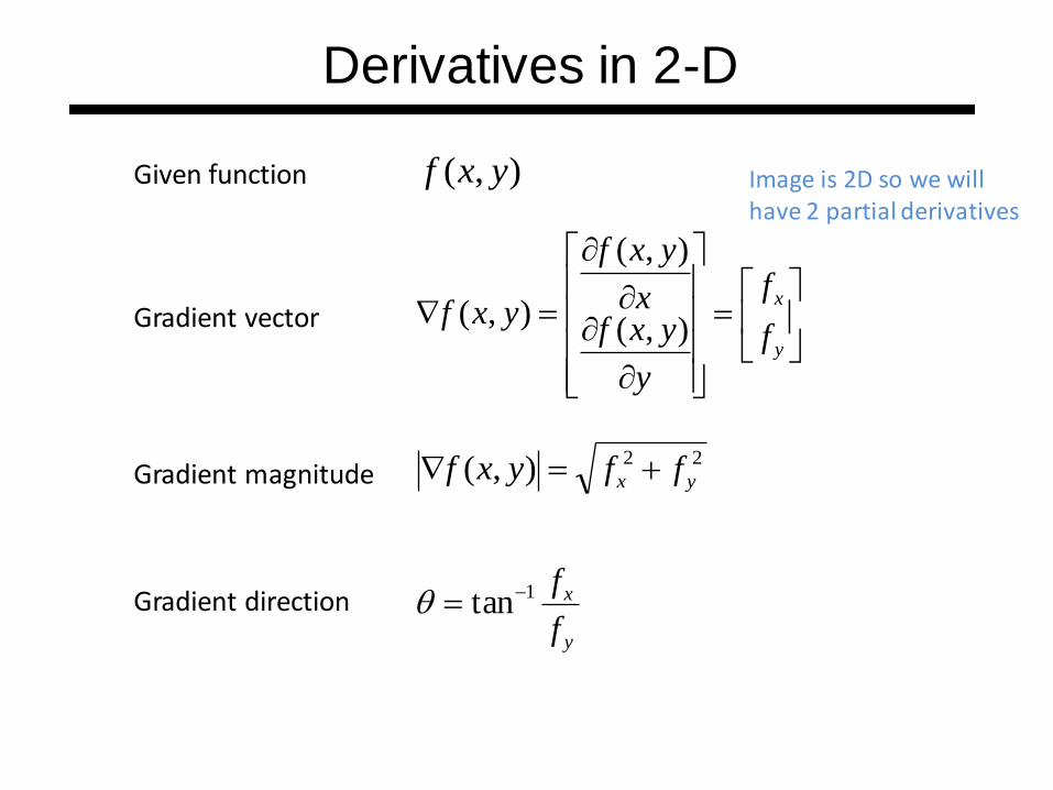
Given function
Gradient vector
Gradient magnitude
Gradient direction
Derivatives in 2-D
Image is 2D so we will have 2 partial derivatives

00000
0010100
0010100
0010100
00000
xI
101
101
101
3
1xfDerivative masks
1 1 11
0 0 03
1 1 1
yf
2020201010
2020201010
2020201010
2020201010
2020201010
I
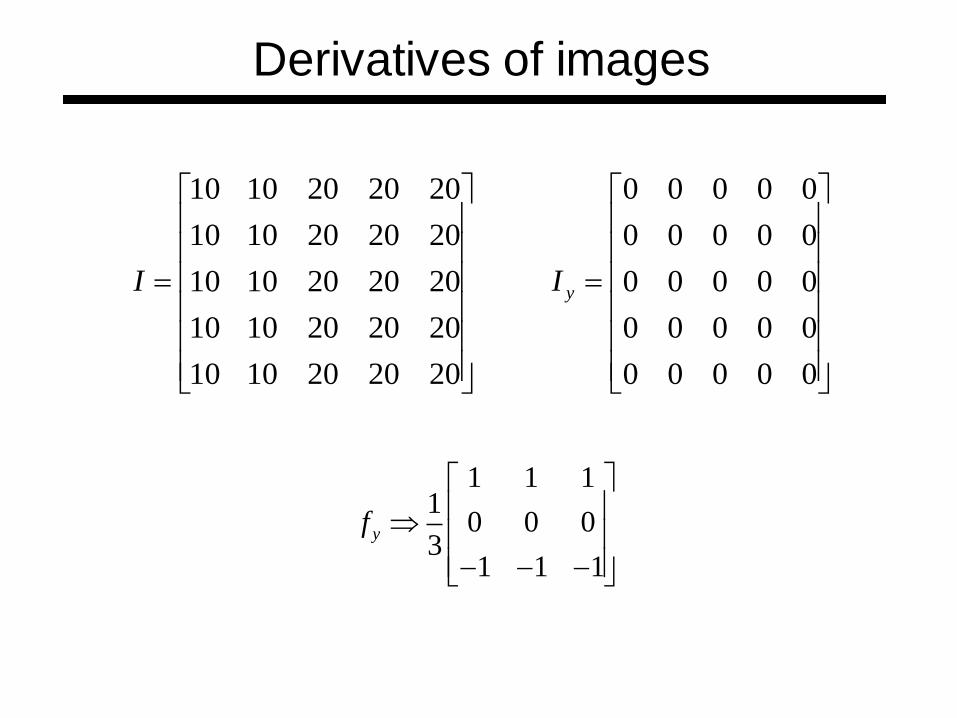
Derivatives of images
Averaging is one way to get rid of noise in any pixel
(-10+0+20) + (-10+0+20) + (-10+0+20) = 30
00000
00000
00000
00000
00000
yI
2020201010
2020201010
2020201010
2020201010
2020201010
I
Derivatives of images
1 1 11
0 0 03
1 1 1
yf

2
2
2)(
x
exg
( ) .011 .13 .6 1 .6 .13 .011g x
2 2
2
( )
2( , )
x y
g x y e
Gaussian Filter
1
x=-3 x=-2 x=-1 x=0 x=1 x=2 x=3

• Most common natural model
• Smooth function, it has infinite number of derivatives
• Fourier Transform of Gaussian is Gaussian
• Convolution of a Gaussian with itself is a Gaussian
• There are cells in eye that perform Gaussian filtering
Properties of Gaussian

• Mean
n
I
n
IIII
n
i
i
n
121
n
Iw
n
IwIwIwI
n
i
ii
nn
12211
Averages
• Weighted mean

Image filtering
• Modify pixels in an image based on some function of a local neighborhood of the pixels
10 5 3
4 5 1
1 1 7
Some function
Local image data Modified image data
7
pf
• Replace each pixel by a linear combination of its neighbors • We don’t want to only do this at a single pixel, of course, but want instead to “run the kernel over the whole image”.

1 1 2 2 3 3
4 4 5 5 6 6
7 7 8 8 9 9
f h f h f h f h
f h f h f h
f h f h f h
( , ) ( , )k l
f h f k l h i k j l
Correlation
f1 f2 f3
f4 f5 f6
f7 f8 f9
f = image h = kernel/filter
h1 h2 h3
h4 h5 h6
h7 h8 h9
Go through each row Given a row, go through each column

1 9 2 8 3 7
4 6 5 5 6 4
7 3 8 2 9 1
*f h f h f h f h
f h f h f h
f h f h f h
* ( , ) ( , )k l
f h f k l h i k j l
Convolution
f1 f2 f3
f4 f5 f6
f7 f8 f9
f = image h = kernel/filter
h9 h8 h7
h6 h5 h4
h3 h2 h1
h1 h2 h3
h4 h5 h6
h7 h8 h9
h7 h8 h9
h4 h5 h6
h1 h2 h3
X-flip
Y-flip If h is symmetric here eg. Gaussian, correlation and convolution will have same results

Lets Start !!!
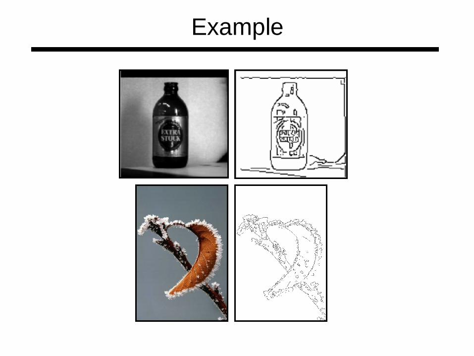
Example

• What is an object?
• How can we find it?
An Application

• Can occur due to different sources
– Shadows
– Texture
Edge Detection in Images
Edges show discontinuity and change in shape and color etc
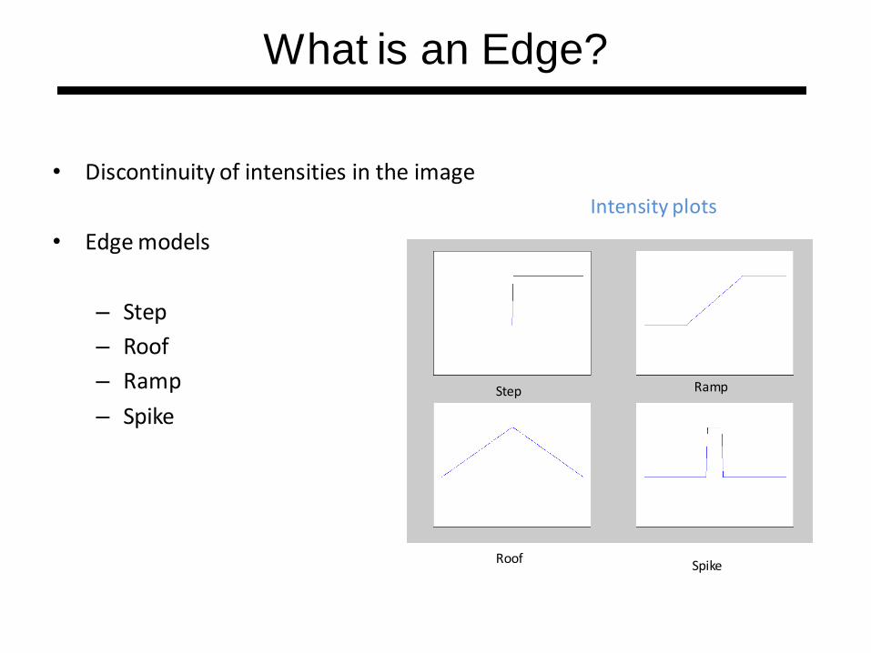
• Discontinuity of intensities in the image
• Edge models
– Step
– Roof
– Ramp
– Spike Step Ramp
Roof Spike
What is an Edge?
Intensity plots
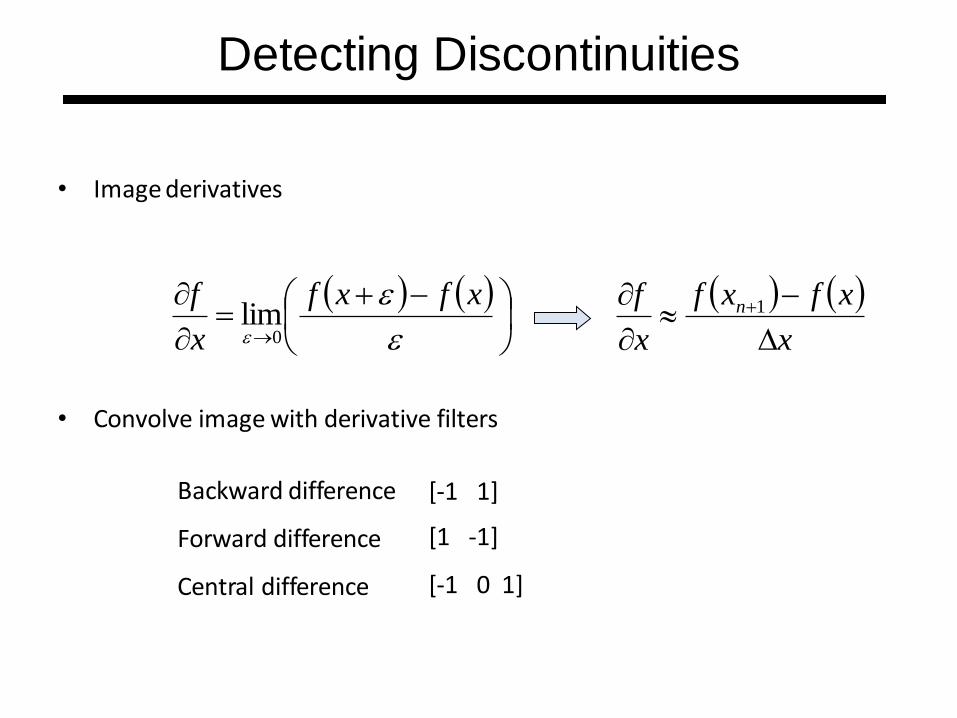
• Image derivatives
• Convolve image with derivative filters
xfxf
x
f
0lim
x
xfxf
x
f n
1
Backward difference
Forward difference
Central difference
[-1 1]
[1 -1]
[-1 0 1]
Detecting Discontinuities

• Definition
• Approximation
• Convolution kernels
yxfyxf
x
yxf ,,lim
,
0
yxfyxf
y
yxf ,,lim
,
0
x
yxfyxf
x
yxf mnmn
,,, 1 1, , ,n m n mf x y f x y f x y
y y
11 xf
1
1yf
Derivative in Two-Dimensions

11* II x
1
1*II yImage I
Image Derivatives

Strongly affected by noise
– obvious reason: image noise results in pixels that look very different from their neighbors
The larger the noise is the stronger the response
What is to be done? – Neighboring pixels look
alike
– Pixel along an edge look alike
– Image smoothing should help Force pixels different to
their neighbors (possibly noise) to look like neighbors
Derivatives and Noise
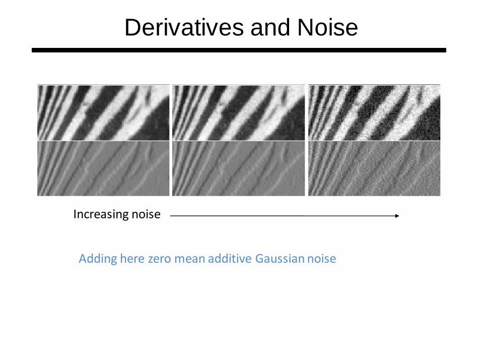
Adding here zero mean additive Gaussian noise
Increasing noise
Derivatives and Noise

• Expect pixels to “be like” their neighbors
– Relatively few reflectance changes
• Generally expect noise to be independent from pixel to pixel
– Smoothing suppresses noise
Image Smoothing

• Scale of Gaussian
– As increases, more pixels are involved in average
– As increases, image is more blurred
– As increases, noise is more effectively suppressed
2 2
2
( )
2( , )
x y
g x y e
Gaussian Smoothing

• Gradient operators
– Prewit
– Sobel
• Laplacian of Gaussian (Marr-Hildreth)
• Gradient of Gaussian (Canny)
Edge Detectors

• Compute derivatives
– In x and y directions
• Find gradient magnitude
• Threshold gradient magnitude
Prewitt and Sobel Edge Detector
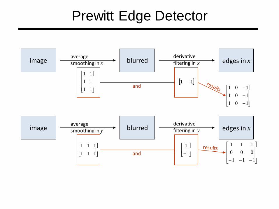
image blurred edges in x average smoothing in x
derivative filtering in x
11
11
11
11
1
1
101
101
101
111
000
111
111
111
and
image blurred edges in x average smoothing in y
derivative filtering in y
and
Prewitt Edge Detector

Image I
101
202
101
121
000
121
*
*
Idx
d
Idy
d
22
I
dy
dI
dx
dThreshold Edges
Sobel Edge Detector
Center row has more weight
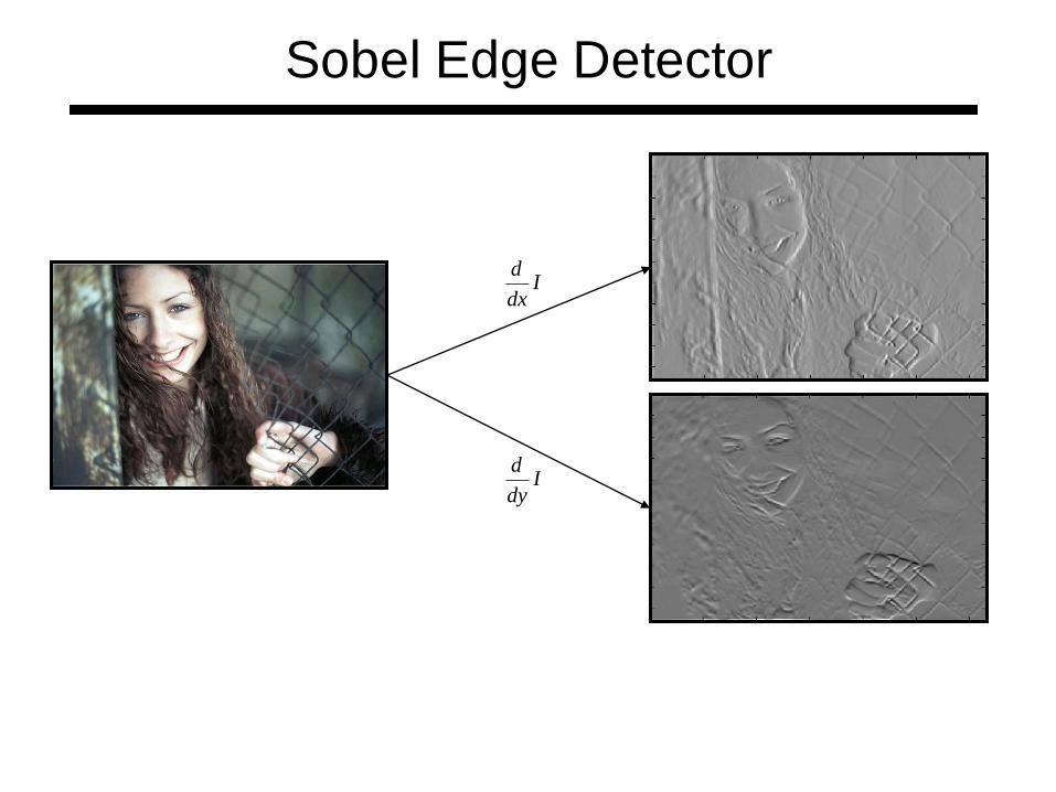
Idx
d
Idy
d
Sobel Edge Detector

22
I
dy
dI
dx
d
100 Threshold
Sobel Edge Detector
Magnitude

• Smooth image by Gaussian filter S
• Apply Laplacian to S
– Used in mechanics, electromagnetics, wave theory, quantum mechanics and Laplace equation
• Find zero crossings and declare edge point
– Scan along each row, record an edge point at the location of zero-crossing
– Repeat above step along each column
Marr Hildreth Edge Detector
Calculus first derivative is maxima and second derivative is a zero
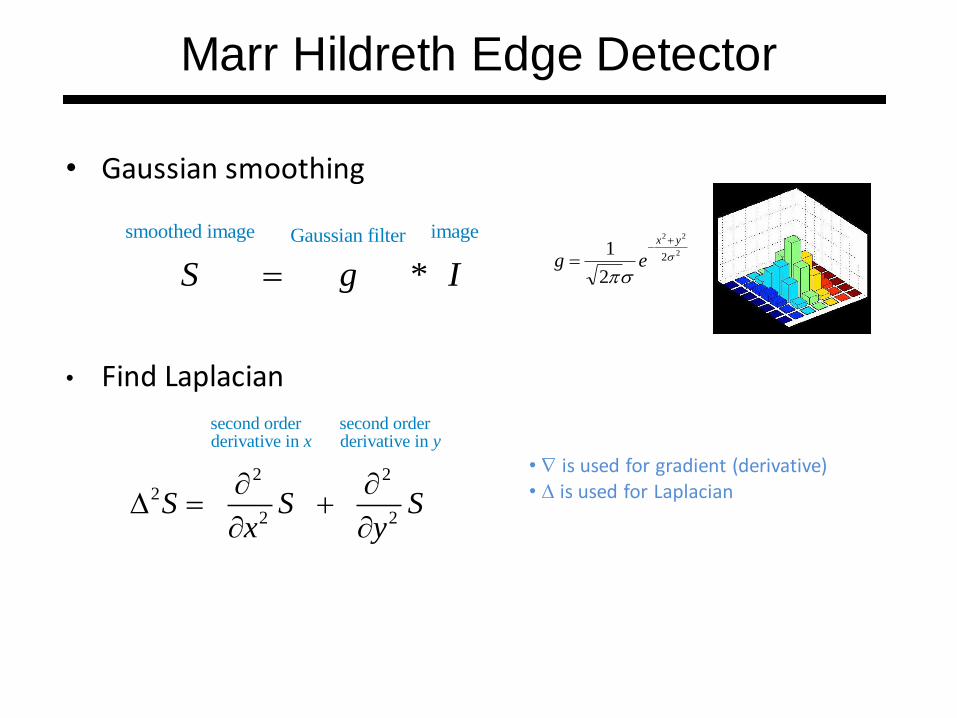
• Gaussian smoothing
smoothed image imageGaussian filter
*S g I2
22
2
2
1
yx
eg
• Find Laplacian
second order second orderderivative in
2 22
2
derivative
2
inx y
S S Sx y
• is used for gradient (derivative) • is used for Laplacian
Marr Hildreth Edge Detector
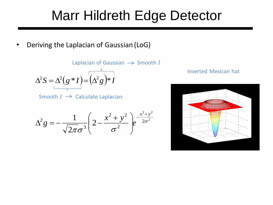
• Deriving the Laplacian of Gaussian (LoG)
IgIgS ** 222
2
22
22
22
3
2 22
1
yx
eyx
g
Marr Hildreth Edge Detector
Inverted Mexican hat
Smooth I Calculate Laplacian
Laplacian of Gaussian Smooth I
2
22
22
22
3
2 22
1
yx
eyx
G
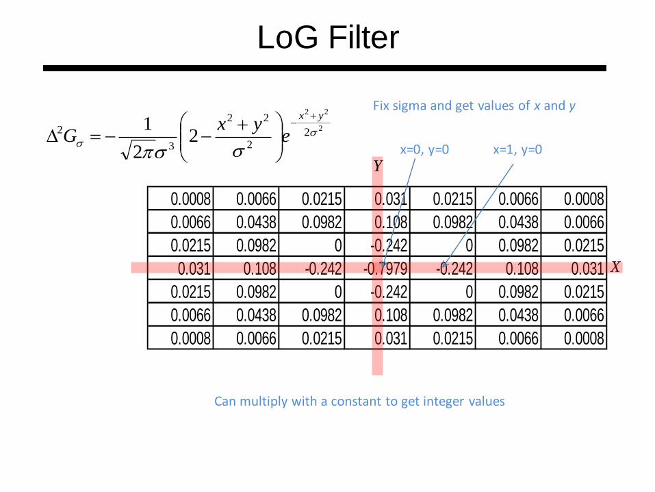
0.0008 0.0066 0.0215 0.031 0.0215 0.0066 0.0008
0.0066 0.0438 0.0982 0.108 0.0982 0.0438 0.0066
0.0215 0.0982 0 -0.242 0 0.0982 0.0215
0.031 0.108 -0.242 -0.7979 -0.242 0.108 0.031
0.0215 0.0982 0 -0.242 0 0.0982 0.0215
0.0066 0.0438 0.0982 0.108 0.0982 0.0438 0.0066
0.0008 0.0066 0.0215 0.031 0.0215 0.0066 0.0008
X
Y
LoG Filter
Can multiply with a constant to get integer values
x=0, y=0
x=1, y=0
Fix sigma and get values of x and y
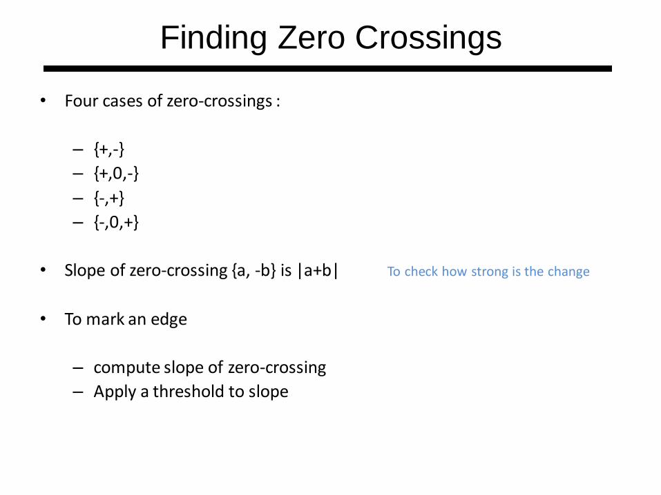
• Four cases of zero-crossings :
– {+,-}
– {+,0,-}
– {-,+}
– {-,0,+}
• Slope of zero-crossing {a, -b} is |a+b|
• To mark an edge
– compute slope of zero-crossing
– Apply a threshold to slope
Finding Zero Crossings
To check how strong is the change
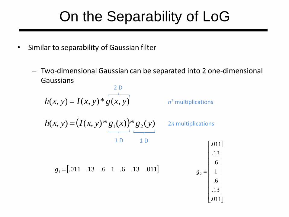
• Similar to separability of Gaussian filter
– Two-dimensional Gaussian can be separated into 2 one-dimensional Gaussians
),(*),(),( yxgyxIyxh
)(*)(*),(),( 21 ygxgyxIyxh
n2 multiplications
2n multiplications
011.13.6.16.13.011.1 g
011.
13.
6.
1
6.
13.
011.
2g
On the Separability of LoG
2 D
1 D 1 D

Requires n2 multiplications
gIIgIgS 2222 ***
2 ( ) ( ) ( ) ( )xx yyS I g x g y I g y g x
Requires 4n multiplications
On the Separability of LoG
4 x 1D convolutions
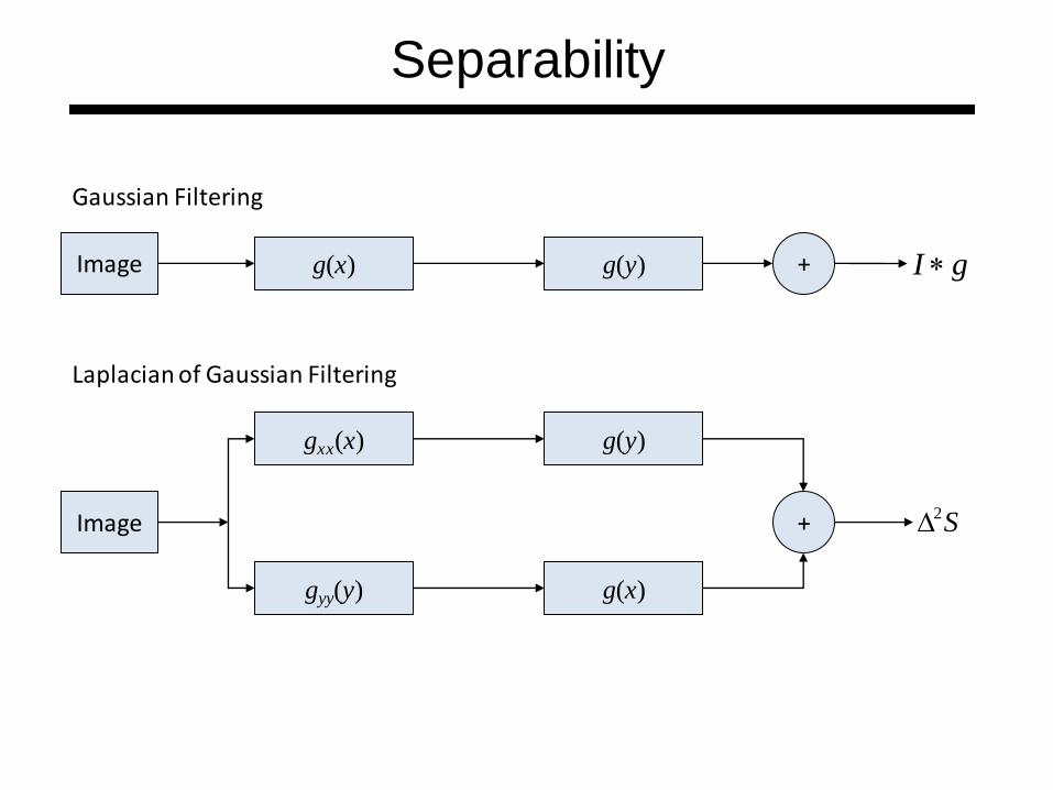
Image
gxx(x) g(y)
gyy(y) g(x)
+ S2
Image g(x) g(y) + gI
Gaussian Filtering
Laplacian of Gaussian Filtering
Separability

gI 2* I S2 of crossings Zero
Example

1
6
3
Example
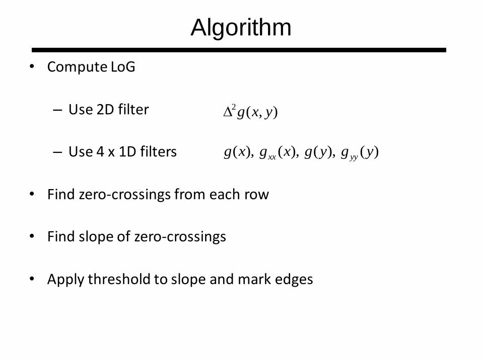
• Compute LoG
– Use 2D filter
– Use 4 x 1D filters
• Find zero-crossings from each row
• Find slope of zero-crossings
• Apply threshold to slope and mark edges
),(2 yxg
)(),(),(),( ygygxgxg yyxx
Algorithm
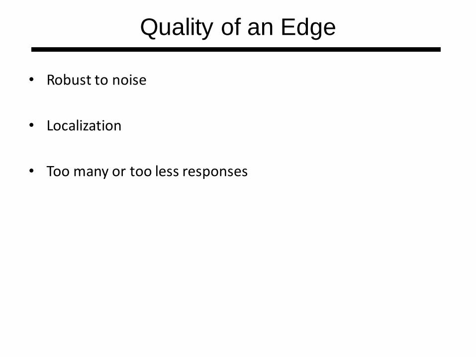
• Robust to noise
• Localization
• Too many or too less responses
Quality of an Edge

True edge
Poor robustness to noise
Poor localization
Too many responses
Quality of an Edge
Edge points

• Prewitt and Sobel edge detectors
– Compute derivatives
• In x and y directions
– Find gradient magnitude
– Threshold gradient magnitude
• Difference between Prewitt and Sobel is the derivative filters
Recap (Prewitt and Sobel)

Prewitt’s edges in x
direction
101
101
101
111
000
111Prewitt’s edges in y
direction
xI
yI
Prewitt Edge Detector
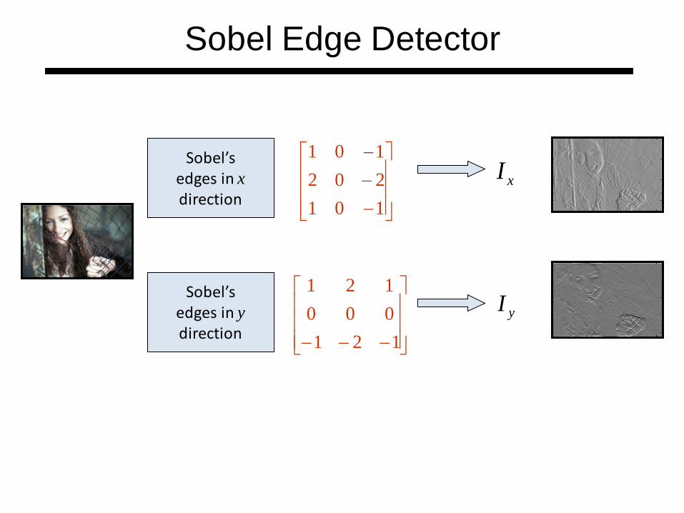
Sobel’s edges in x
direction
101
202
101
121
000
121Sobel’s edges in y
direction
xI
yI
Sobel Edge Detector
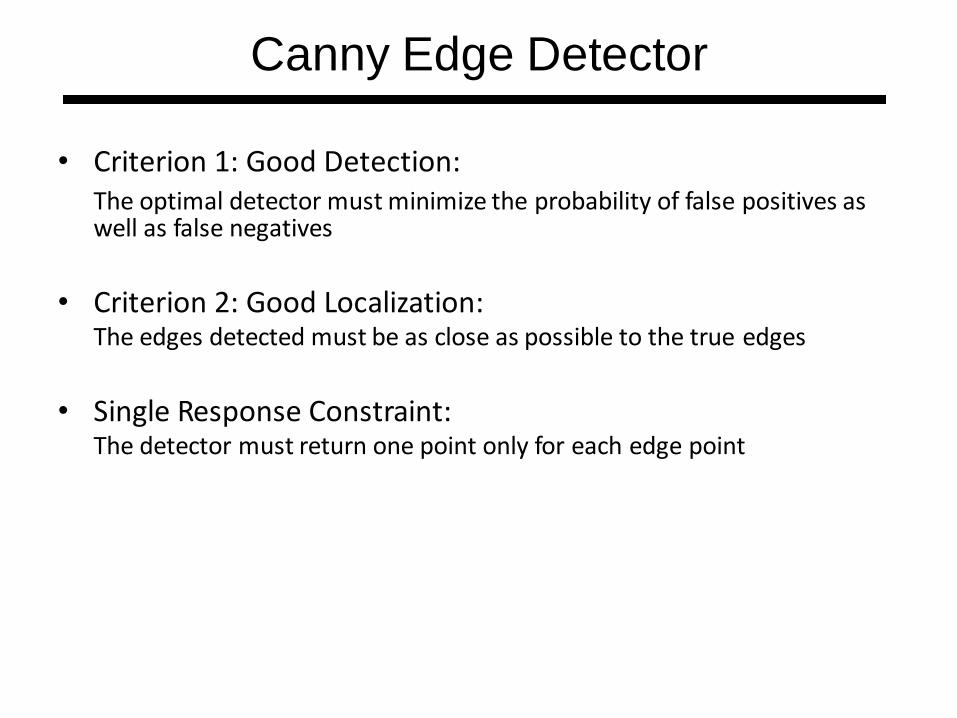
• Criterion 1: Good Detection: The optimal detector must minimize the probability of false positives as
well as false negatives
• Criterion 2: Good Localization: The edges detected must be as close as possible to the true edges
• Single Response Constraint: The detector must return one point only for each edge point
Canny Edge Detector
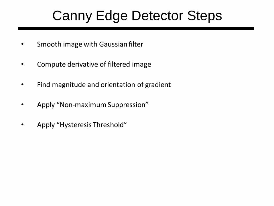
• Smooth image with Gaussian filter
• Compute derivative of filtered image
• Find magnitude and orientation of gradient
• Apply “Non-maximum Suppression”
• Apply “Hysteresis Threshold”
Canny Edge Detector Steps

• Smoothing
• Derivative
IyxgyxgIS ),(),(
2
22
2
2
1),(
yx
eyxg
IgIgS
y
x
g
g
y
gx
g
g
Ig
gS
y
x
Ig
Ig
y
x
Canny Edge Detector - First Two Steps

),( yxg
),( yxgx
),( yxg y
Canny Edge Detector - Derivative of Gaussian

xS
yS
I
Canny Edge Detector - First Two Steps
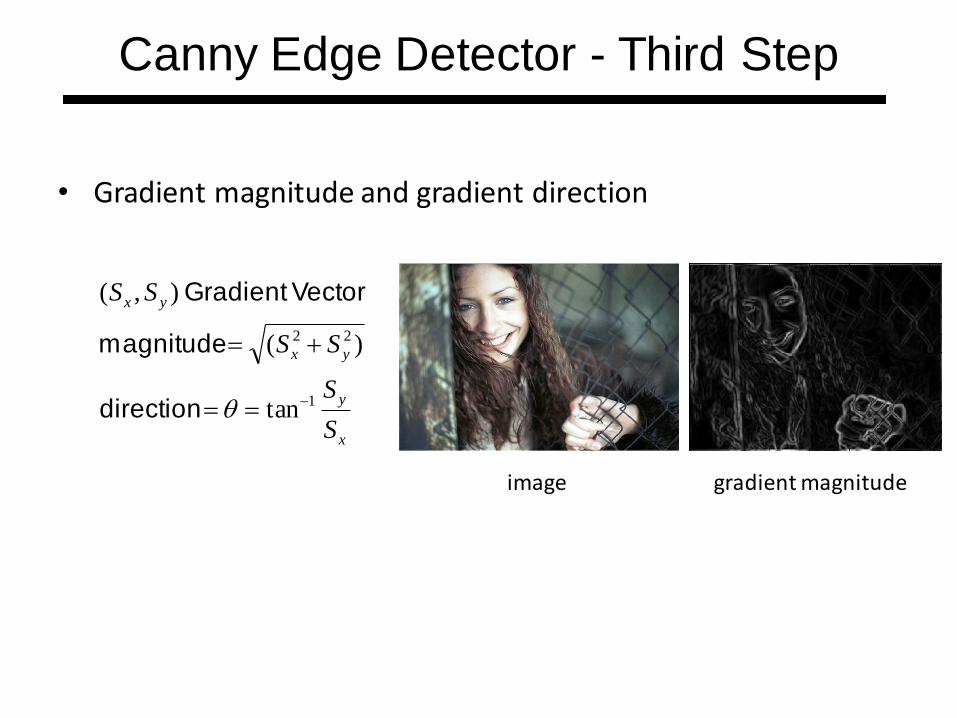
• Gradient magnitude and gradient direction
x
y
yx
yx
S
S
SS
SS
1
22
tan
)(
),(
direction
magnitude
VectorGradient
image gradient magnitude
Canny Edge Detector - Third Step

• Non maximum suppression
We wish to mark points along the curve where the magnitude is biggest. We can do this by looking for a maximum along a slice normal to the curve (non-maximum suppression). These points should form a curve. There are then two algorithmic issues: at which point is the maximum, and where is the next one?
Canny Edge Detector - Fourth Step
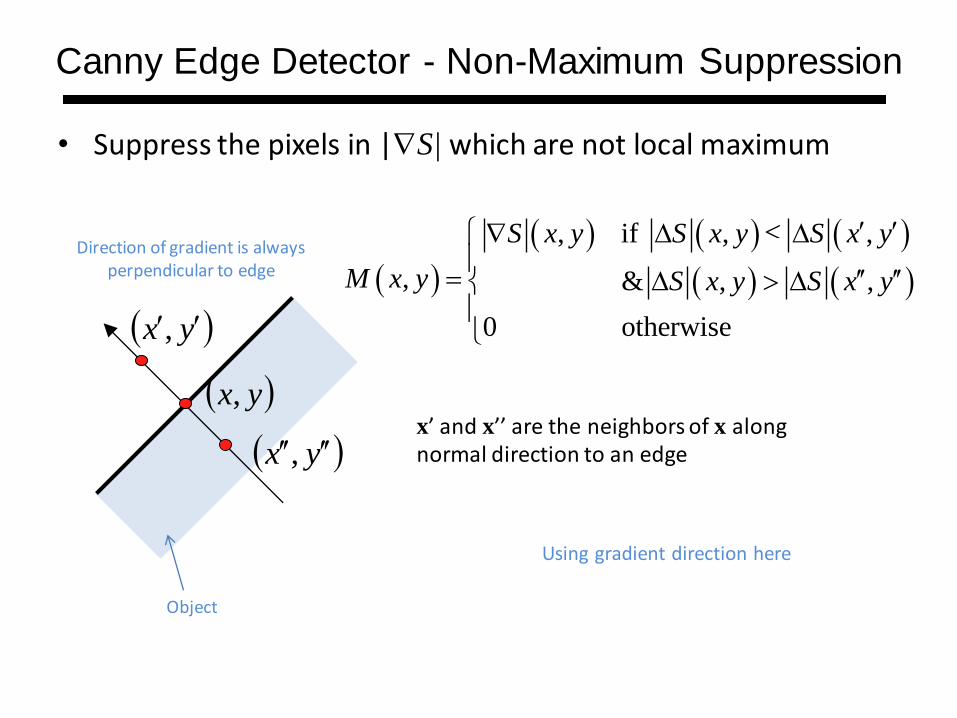
• Suppress the pixels in |S| which are not local maximum
, if , ,
, & , ,
0 otherwise
S x y S x y S x y
M x y S x y S x y
x’ and x’’ are the neighbors of x along normal direction to an edge
Canny Edge Detector - Non-Maximum Suppression
yx ,
yx,
yx ,
Direction of gradient is always perpendicular to edge
Object
Using gradient direction here

22
yx SSS M
25ThresholdM
ionvisualizat For
Canny Edge Detector - Non-Maximum Suppression
Magnitude after Non-Maximum Suppression
Magnitude
Further Thresholding

• If the gradient at a pixel is
– above “High”, declare it an ‘edge pixel’
– below “Low”, declare it a “non-edge-pixel”
– between “low” and “high”
• Consider its neighbors iteratively then declare it an “edge pixel” if it is connected to an ‘edge pixel’ directly or via pixels between “low” and “high”.
Canny Edge Detector - Hysteresis Thresholding
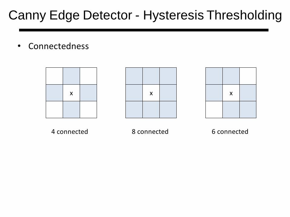
• Connectedness
x x x
4 connected 8 connected 6 connected
Canny Edge Detector - Hysteresis Thresholding
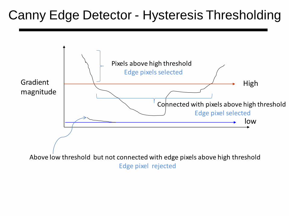
High
low
Gradient magnitude
Canny Edge Detector - Hysteresis Thresholding
Pixels above high threshold Edge pixels selected
Connected with pixels above high threshold Edge pixel selected
Above low threshold but not connected with edge pixels above high threshold Edge pixel rejected
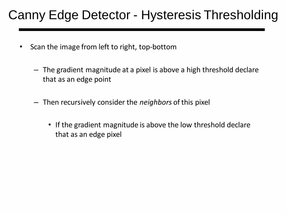
• Scan the image from left to right, top-bottom
– The gradient magnitude at a pixel is above a high threshold declare that as an edge point
– Then recursively consider the neighbors of this pixel
• If the gradient magnitude is above the low threshold declare that as an edge pixel
Canny Edge Detector - Hysteresis Thresholding

M 25M
regular
15
35
Hysteresis
Low
High
Canny Edge Detector - Hysteresis Thresholding

???
Final project ideas!!!
I will upload the list this week

Will be uploaded
Assignment 01
Next class
Quiz 01


