Download - EE360: SIGNALS AND SYSTEMS - UNLV

http://www.ee.unlv.edu/~b1morris/ee360
EE360: SIGNALS AND SYSTEMS
CH3: FOURIER SERIES
1

FOURIER SERIES OVERVIEW, MOTIVATION, AND HIGHLIGHTSCHAPTER 3.1-3.2
2

BIG IDEA: TRANSFORM ANALYSIS
Make use of properties of LTI systems to simplify analysis
Represent signals as a linear combination of basic signals with two properties
Simple response: easy to characterize LTI system response to basic signal
Representation power: the set of basic signals can be use to construct a broad/useful class of signals
3

When plucking a string, length is divided into integer divisions or harmonics
Frequency of each harmonic is an integer multiple of a “fundamental frequency”
Also known as the normal modes
Any string deflection could be built out of a linear combination of “modes”
4
NORMAL MODES OF VIBRATING STRING

When plucking a string, length is divided into integer divisions or harmonics
Frequency of each harmonic is an integer multiple of a “fundamental frequency”
Also known as the normal modes
Any string deflection could be built out of a linear combination of “modes”
5
NORMAL MODES OF VIBRATING STRING
Caution: turn your sound down
https://youtu.be/BSIw5SgUirg

Fourier argued that periodic signals (like the single period from a plucked string) were actually useful
Represent complex periodic signals
Examples of basic periodic signals
Sinusoid: 𝑥 𝑡 = 𝑐𝑜𝑠𝜔0𝑡
Complex exponential: 𝑥 𝑡 = 𝑒𝑗𝜔0t
Fundamental frequency: 𝜔0
Fundamental period: 𝑇 =2𝜋
𝜔0
Harmonically related period signals form family
Integer multiple of fundamental frequency
𝜙𝑘 𝑡 = 𝑒𝑗𝑘𝜔0𝑡 for 𝑘 = 0,±1,±2,…
Fourier Series is a way to represent a periodic signal as a linear combination of harmonics
𝑥 𝑡 = σ𝑘=−∞∞ 𝑎𝑘𝑒
𝑗𝑘𝜔0𝑡
𝑎𝑘 coefficient gives the contribution of a harmonic (periodic signal of 𝑘times frequency)
6
FOURIER SERIES 1 SLIDE OVERVIEW

SAWTOOTH EXAMPLE
7
signalHarmonics: height given by coefficient
Animation showing approximation as more harmonics added
𝑎1
𝑎2
𝑎3𝑎4…

SQUARE WAVE EXAMPLE
Better approximation of square wave with more coefficients
Aligned approximations
Animation of FS
8
1
2
3
4
Note: 𝑆(𝑓) ~ 𝑎𝑘
#𝑎𝑘
coef
fici
ents

ARBITRARY EXAMPLES
Interactive examples [flash (dated)][html]
9

RESPONSE OF LTI SYSTEMS TO COMPLEX EXPONENTIALS CHAPTER 3.2
10

TRANSFORM ANALYSIS OBJECTIVE
Need family of signals 𝑥𝑘 𝑡 that have 1) simple response and 2) represent a broad (useful) class of signals
1. Family of signals Simple response – every signal in family pass through LTI system with scale change
2. “Any” signal can be represented as a linear combination of signals in the family
Results in an output generated by input 𝑥(𝑡)
11
𝑥𝑘(𝑡) ⟶ 𝜆𝑘𝑥𝑘(𝑡)
𝑥 𝑡 =
𝑘=−∞
∞
𝑎𝑘𝑥𝑘(𝑡)
𝑥 𝑡 ⟶
𝑘=−∞
∞
𝑎𝑘𝜆𝑘𝑥𝑘(𝑡)

IMPULSE AS BASIC SIGNAL
Previously (Ch2), we used shifted and scaled deltas
𝛿 𝑡 − 𝑡0 ⟹ 𝑥 𝑡 = ∫ 𝑥 𝜏 𝛿 𝑡 − 𝜏 𝑑𝜏 ⟶ 𝑦 𝑡 = ∫ 𝑥 𝜏 ℎ 𝑡 − 𝜏 𝑑𝜏
Thanks to Jean Baptiste Joseph Fourier in the early 1800s we got Fourier analysis
Consider signal family of complex exponentials
𝑥 𝑡 = 𝑒𝑠𝑡 or 𝑥 𝑛 = 𝑧𝑛, 𝑠, 𝑧 ∈ ℂ
12

Using the convolution
𝑒𝑠𝑡 ⟶𝐻 𝑠 𝑒𝑠𝑡
𝑧𝑛 ⟶𝐻 𝑧 𝑧𝑛
Notice the eigenvalue 𝐻 𝑠depends on the value of ℎ(𝑡)and 𝑠
Transfer function of LTI system
Laplace transform of impulse response
13
COMPLEX EXPONENTIAL AS EIGENSIGNAL

TRANSFORM OBJECTIVE
Simple response
𝑥 𝑡 = 𝑒𝑠𝑡 ⟶ 𝑦 𝑡 = 𝐻 𝑠 𝑥 𝑡
Useful representation?
𝑥 𝑡 = σ𝑎𝑘𝑒𝑠𝑘𝑡 ⟶ 𝑦 𝑡 = σ𝑎𝑘𝐻 𝑠𝑘 𝑒𝑠𝑘𝑡
Input linear combination of complex exponentials leads to output linear combination of complex exponentials
Fourier suggested limiting to subclass of period complex exponentials 𝑒𝑗𝑘𝜔0𝑡 , 𝑘 ∈ ℤ,𝜔0 ∈ ℝ
𝑥 𝑡 = σ𝑎𝑘𝑒𝑗𝑘𝜔0𝑡 ⟶ 𝑦 𝑡 = σ𝑎𝑘𝐻 𝑗𝑘𝜔0 𝑒𝑠𝑘𝑡
Periodic input leads to periodic output.
𝐻 𝑗𝜔 = 𝐻 𝑠 ȁ𝑠=𝑗𝜔 is the frequency response of the system
14
CONTINUOUS TIME FOURIER SERIESCHAPTER 3.3-3.8
15
CTFS TRANSFORM PAIR
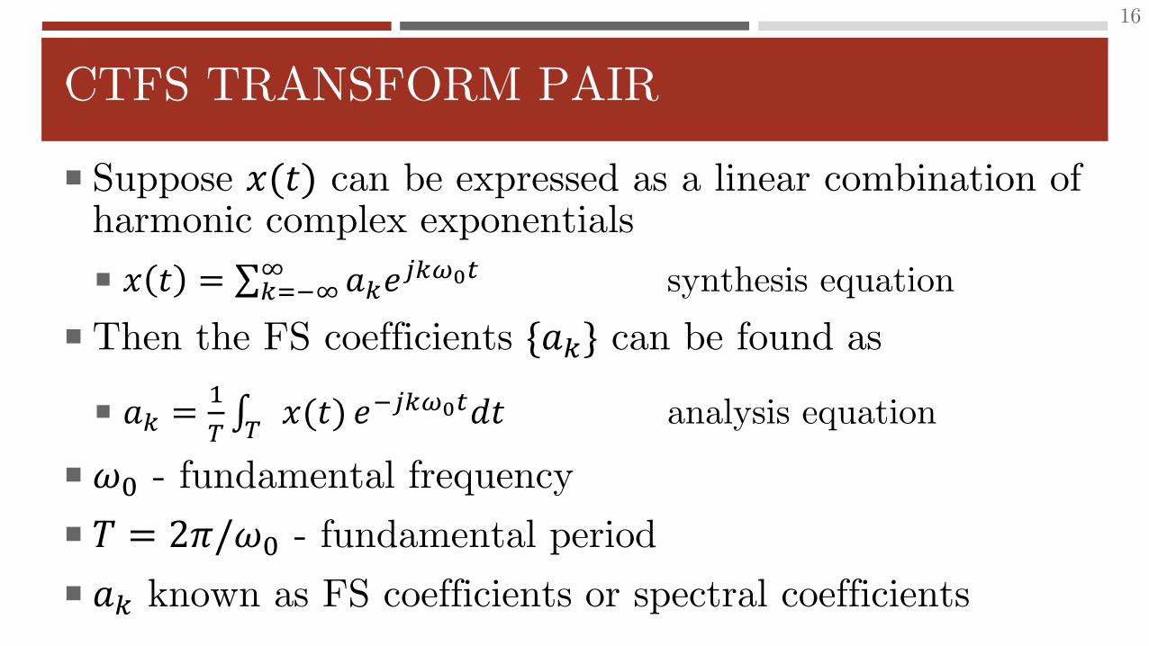
Suppose 𝑥(𝑡) can be expressed as a linear combination of harmonic complex exponentials
𝑥 𝑡 = σ𝑘=−∞∞ 𝑎𝑘𝑒
𝑗𝑘𝜔0𝑡 synthesis equation
Then the FS coefficients {𝑎𝑘} can be found as
𝑎𝑘 =1
𝑇∫𝑇 𝑥(𝑡) 𝑒−𝑗𝑘𝜔0𝑡𝑑𝑡 analysis equation
𝜔0 - fundamental frequency
𝑇 = 2𝜋/𝜔0 - fundamental period
𝑎𝑘 known as FS coefficients or spectral coefficients
16

CTFS PROOF
While we can prove this, it is not well suited for slides.
Key observation from proof: Complex exponentials are orthogonal
17

18
VECTOR SPACE OF PERIODIC SIGNALS
All signals
Periodic signals, 𝜔0

Each of the harmonic exponentials are orthogonal to each other and span the space of periodic signals
The projection of 𝑥(𝑡) onto a particular harmonic (𝑎𝑘) gives the contribution of that complex exponential to building 𝑥 𝑡
𝑎𝑘 is how much of each harmonic is required to construct the periodic signal 𝑥(𝑡)
19
VECTOR SPACE OF PERIODIC SIGNALS
Periodic signals, 𝜔0
𝑥(𝑡)
𝑒𝑗0𝑡 = 1𝑎0
𝑒𝑗(−𝜔0)𝑡
𝑒𝑗𝜔0𝑡
𝑒𝑗2𝜔0𝑡
𝑒𝑗𝑘𝜔0𝑡
𝑎−1
𝑎1
𝑎2
𝑎𝑘

HARMONICS
𝑘 = ±1 ⇒ fundamental component (first harmonic)
Frequency 𝜔0, period 𝑇 = 2𝜋/𝜔0
𝑘 = ±2 ⇒ second harmonic
Frequency 𝜔2 = 2𝜔0, period 𝑇2 = 𝑇/2 (half period)
…
𝑘 = ±𝑁 ⇒ Nth harmonic
Frequency 𝜔𝑁 = 𝑁𝜔0, period 𝑇𝑁 = 𝑇/𝑁 (1/N period)
𝑘 = 0 ⇒ 𝑎0 =1
𝑇∫𝑇 𝑥 𝑡 𝑑𝑡, DC, constant component, average
over a single period
20
HOW TO FIND FS REPRESENTATION
Will use important examples to demonstrate common techniques
Sinusoidal signals – Euler’s relationship
Direct FS integral evaluation
FS properties table and transform pairs
21

𝑥 𝑡 = 1 +1
2cos 2𝜋𝑡 + sin 3𝜋𝑡
First find the period
Constant 1 has arbitrary period
cos 2𝜋𝑡 has period 𝑇1 = 1
sin 3𝜋𝑡 has period 𝑇2 = 2/3
𝑇 = 2, 𝜔0 = 2𝜋/𝑇 = 𝜋
Rewrite 𝑥 𝑡 using Euler’s and read off 𝑎𝑘coefficients by inspection
𝑥 𝑡 = 1 +1
4𝑒𝑗2𝜔0𝑡 + 𝑒−𝑗2𝜔0𝑡 +
1
2𝑗𝑒𝑗3𝜔0𝑡 − 𝑒−𝑗3𝜔0𝑡
Read off coeff. directly
𝑎0 = 1
𝑎1 = 𝑎−1 = 0
𝑎2 = 𝑎−2 = 1/4
𝑎3 = 1/2𝑗, 𝑎−3 = −1/2𝑗
𝑎𝑘 = 0, else
22
SINUSOIDAL SIGNAL

𝑥 𝑡 = ቐ1 𝑡 < 𝑇1
0 𝑇1 < 𝑡 <𝑇
2
23
PERIODIC RECTANGLE WAVE

Important signal/function in DSP and communication
sinc 𝑥 =sin 𝜋𝑥
𝜋𝑥normalized
sinc 𝑥 =sin 𝑥
𝑥unnormalized
Modulated sine function
Amplitude follows 1/x
Must use L’Hopital’s rule to get 𝑥 = 0 time
24
SINC FUNCTION

Consider different “duty cycle” for the rectangle wave
𝑇 = 4𝑇1 50% (square wave)
𝑇 = 8𝑇1 25%
𝑇 = 16𝑇1 12.5%
Note all plots are still a sincshape
Difference is how the sync is sampled
Longer in time (larger T) smaller spacing in frequency more samples between zero crossings
25
RECTANGLE WAVE COEFFICIENTS

Special case of rectangle wave with 𝑇 = 4𝑇1
One sample between zero-crossing
𝑎𝑘 = ቐ1/2 𝑘 = 0
sin(𝑘𝜋/2)
𝑘𝜋𝑒𝑙𝑠𝑒
26
SQUARE WAVE

𝑥 𝑡 = σ𝑘=−∞∞ 𝛿(𝑡 − 𝑘𝑇)
Using FS integral
Notice only one impulse in the interval
27
PERIODIC IMPULSE TRAIN
PROPERTIES OF CTFS
Since these are very similar between CT and DT, will save until after DT
Properties are used to avoid direct evaluation of FS integral
Be sure to bookmark properties in Table 3.1 on page 206
28

DISCRETE TIME FOURIER SERIESCHAPTER 3.6
29

DTFS VS CTFS DIFFERENCES
While quite similar to the CT case,
DTFS is a finite series, 𝑎𝑘 , k < K
Does not have convergence issues
Good News: motivation and intuition from CT applies for DT case
30

DTFS TRANSFORM PAIR
Consider the discrete time periodic signal 𝑥 𝑛 = 𝑥 𝑛 + 𝑁
𝑥 𝑛 = σ𝑘=<𝑁> 𝑎𝑘𝑒𝑗𝑘𝜔0𝑛 synthesis equation
𝑎𝑘 =1
𝑁σ𝑛=<𝑁> 𝑥 𝑛 𝑒−𝑗𝑘𝜔0𝑛 analysis equation
𝑁 – fundamental period (smallest value such that periodicity constraint holds)
𝜔0 = 2𝜋/𝑁 – fundamental frequency
σ𝑛=<𝑁> indicates summation over a period (𝑁 samples)
31

DTFS REMARKS
DTFS representation is a finite sum, so there is always pointwise convergence
FS coefficients are periodic with period N
32

DTFS PROOF
Proof for the DTFS pair is similar to the CT case
Relies on orthogonality of harmonically related DT period complex exponentials
Will not show in class
33

HOW TO FIND DTFS REPRESENTATION
Like CTFS, will use important examples to demonstrate common techniques
Sinusoidal signals – Euler’s relationship
Direct FS summation evaluation – periodic rectangular wave and impulse train
FS properties table and transform pairs
34

𝑥[𝑛] = 1 +1
2cos
2𝜋
𝑁𝑛 + sin
4𝜋
𝑁𝑛
First find the period
Rewrite 𝑥[𝑛] using Euler’s and read off 𝑎𝑘 coefficients by inspection
Shortcut here
𝑎0 = 1, 𝑎±1 =1
4, 𝑎2 = 𝑎−2
∗ =1
2𝑗
35
SINUSOIDAL SIGNAL
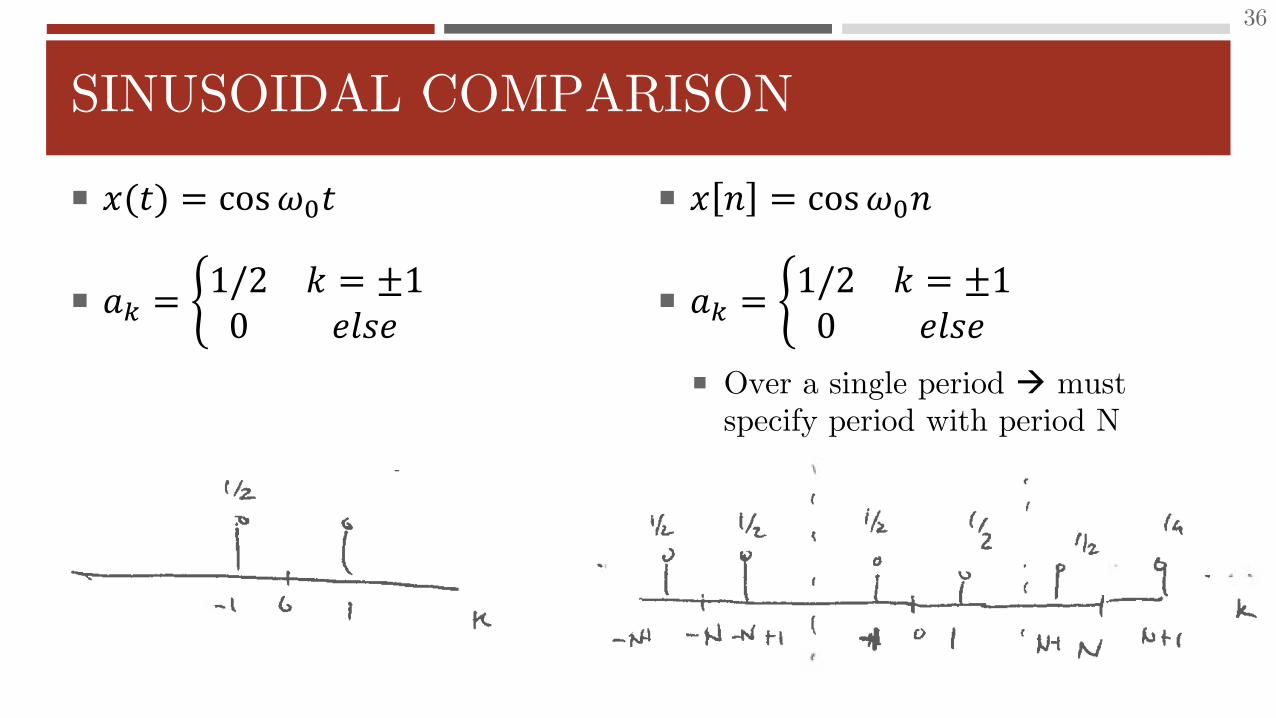
𝑥(𝑡) = cos𝜔0𝑡
𝑎𝑘 = ቊ1/2 𝑘 = ±10 𝑒𝑙𝑠𝑒
𝑥 𝑛 = cos𝜔0𝑛
𝑎𝑘 = ቊ1/2 𝑘 = ±10 𝑒𝑙𝑠𝑒
Over a single period must specify period with period N
36
SINUSOIDAL COMPARISON
Type equation here.
37
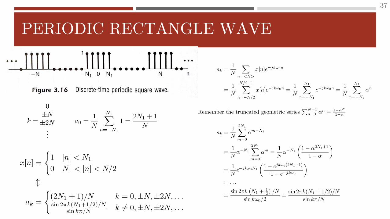
PERIODIC RECTANGLE WAVE

Consider different “duty cycle” for the rectangle wave
50% (square wave)
25%
12.5%
Note all plots are still a sincshaped, but periodic
Difference is how the sync is sampled
Longer in time (larger N) smaller spacing in frequency more samples between zero crossings
38
RECTANGLE WAVE COEFFICIENTS

𝑥[𝑛] = σ𝑘=−∞∞ 𝛿[𝑛 − 𝑘𝑁]
Using FS integral
Notice only one impulse in the interval
39
PERIODIC IMPULSE TRAIN

PROPERTIES OF FOURIER SERIESCHAPTER 3.5, 3.7
40
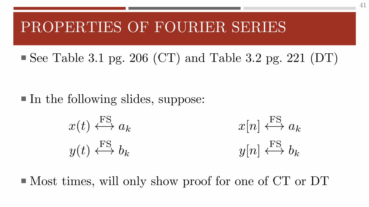
PROPERTIES OF FOURIER SERIES
See Table 3.1 pg. 206 (CT) and Table 3.2 pg. 221 (DT)
In the following slides, suppose:
Most times, will only show proof for one of CT or DT
41

CT
𝐴𝑥 𝑡 + 𝐵𝑦 𝑡 ⟷ 𝐴𝑎𝑘 + 𝐵𝑏𝑘
DT
𝐴𝑥 𝑛 + 𝐵𝑦 𝑛 ⟷ 𝐴𝑎𝑘 + 𝐵𝑏𝑘
42
LINEARITY

CT
𝑥(𝑡 − 𝑡0) ⟷ 𝑎𝑘𝑒−𝑗𝑘𝜔0𝑡0
Proof
Let 𝑦 𝑡 = 𝑥(𝑡 − 𝑡0)
DT
𝑥[𝑛 − 𝑛0] ⟷ 𝑎𝑘𝑒−𝑗𝑘𝜔0𝑛0
43
TIME-SHIFT

CT
𝑒𝑗𝑀𝜔0𝑡𝑥 𝑡 ⟷ 𝑎𝑘−𝑀
DT
𝑒𝑗𝑀𝜔0𝑛𝑥 𝑛 ⟷ 𝑎𝑘−𝑀
44
FREQUENCY SHIFT
Note: Similar relationship with Time Shift (dualilty). Multiplication by exponential in time is a shift in frequency. Shift in time is a multiplication by exponential in frequency.

CT
𝑥(−𝑡) ⟷ 𝑎−𝑘
DT
𝑥[−𝑛] ⟷ 𝑎−𝑘
45
TIME REVERSAL

CT
∫𝑇 𝑥 𝜏 𝑦 𝑡 − 𝜏 𝑑𝜏 ⟷ 𝑇𝑎𝑘𝑏𝑘
DT
σ𝑟=<𝑁> 𝑥 𝑟 𝑦[𝑛 − 𝑟] ⟷ 𝑁𝑎𝑘𝑏𝑘
46
PERIODIC CONVOLUTION

CT
𝑥 𝑡 𝑦(𝑡) ⟷ σ𝑙=−∞∞ 𝑎𝑙𝑏𝑘−𝑙 = 𝑎𝑘 ∗ 𝑏𝑘
DT
𝑥 𝑛 𝑦[𝑛] ⟷ σ𝑙=<𝑁>𝑎𝑙𝑏𝑘−𝑙 = 𝑎𝑘 ∗ 𝑏𝑘
Convolution over a single period (DT FS is periodic)
47
MULTIPLICATION
Note: Similar relationship with Convolution (dualilty). Convolution in time results in multiplication in frequency domain. Multiplication in time results in convolution in frequency domain.

CT
1
𝑇∫𝑇 𝑥 𝑡 2𝑑𝑡 = σ𝑘=−∞
∞ 𝑎𝑘2
DT
1
𝑁σ𝑛=<𝑁> 𝑥 𝑛 2 = σ𝑘=<𝑁> 𝑎𝑘
2
48
PARSEVAL’S RELATION
Note: Total average power in a periodic signal equals the sum of the average power in all its harmonic components
1
Tන𝑇
𝑎𝑘𝑒𝑗𝑘𝜔0𝑡
2𝑑𝑡 =
1
𝑇න𝑇
𝑎𝑘2𝑑𝑡 = 𝑎𝑘
2
Average power in the 𝑘th harmonic

CT
𝑥(𝛼𝑡) ⟷ 𝑎𝑘
𝛼 > 0
Periodic with period 𝑇/𝛼
DT
𝑥(𝑚) 𝑛 = ቊ𝑥[𝑛/𝑚] 𝑛 multiple of 𝑚
0 𝑒𝑙𝑠𝑒
Periodic with period 𝑚𝑁
𝑥(𝑚)[𝑛] ⟷1
𝑚𝑎𝑘
Periodic with period 𝑚𝑁
49
TIME SCALING
Note: Not all properties are exactly the same. Must be careful due to constraints on periodicity for DT signal.

FOURIER SERIES AND LTI SYSTEMSCHAPTER 3.8
50

EIGENSIGNAL REMINDER
𝑥 𝑡 = 𝑒𝑠𝑡 ⟷ 𝑦 𝑡 = 𝐻 𝑠 𝑒𝑠𝑡 𝑥 𝑛 = 𝑧𝑛 ⟷ 𝑦 𝑛 = 𝐻 𝑧 𝑧𝑛
𝐻 𝑠 = ∫−∞∞ℎ 𝑡 𝑒−𝑠𝑡𝑑𝑡 𝐻 𝑧 = σ𝑛=−∞
∞ ℎ 𝑛 𝑧−𝑘
𝐻 𝑠 ,𝐻 𝑧 known as system function (𝑠, 𝑧 ∈ ℂ)
For Fourier Analysis (e.g. FS)
Let 𝑠 = 𝑗𝜔 and 𝑧 = 𝑒𝑗𝜔
Frequency response (system response to particular input frequency)
𝐻 𝑗𝜔 = 𝐻 𝑠 ȁ𝑠=𝑗𝜔 = ∫−∞∞ℎ 𝑡 𝑒−𝑗𝜔𝑡𝑑𝑡
𝐻 𝑒𝑗𝜔 = 𝐻 𝑧 ȁ𝑧=𝑒𝑗𝜔 = σ𝑛=−∞∞ ℎ 𝑛 𝑒−𝑗𝜔𝑛
51

FOURIER SERIES AND LTI SYSTEMS I
Consider now a FS representation of a periodic signals
𝑥 𝑡 = σ𝑘 𝑎𝑘𝑒𝑗𝑘𝜔0𝑡
→ 𝑦 𝑡 = σ𝑘 𝑎𝑘𝐻 𝑗𝑘𝜔0 𝑒𝑗𝑘𝜔0𝑡
Due to superposition (LTI system)
Each harmonic in results in harmonic out with eigenvalue
𝑦(𝑡) periodic with same fundamental frequency as 𝑥(𝑡) ⇒ 𝜔0
𝑇 =2𝜋
𝜔0- fundamental period
FS coefficients for 𝑦 𝑡
𝑏𝑘 = 𝑎𝑘𝐻(𝑗𝑘𝜔0)
𝑏𝑘 is the FS coefficient 𝑎𝑘 multiplied/affected by frequency response at 𝑘𝜔0
52

FOURIER SERIES AND LTI SYSTEMS III
System block diagram
53
𝑎−𝑘𝑒−𝑗𝑘𝜔0𝑡 𝐻(𝑗𝜔)
𝑥 𝑡 =
𝑦(𝑡)𝑎0𝑒𝑗(0)𝜔0𝑡 𝐻(𝑗𝜔)
𝑎𝑘𝑒𝑗𝑘𝜔0𝑡 𝐻(𝑗𝜔)
⋮
⋮
𝑎−𝑘𝐻(−𝑗𝑘𝜔0)𝑒−𝑗𝑘𝜔0𝑡
𝑎𝑘𝐻(𝑗𝑘𝜔0)𝑒−𝑗𝑘𝜔0𝑡
𝑎0𝐻(−𝑗0)

DTFS AND LTI SYSTEMS
𝑥 𝑛 = σ𝑘=<𝑁>𝑎𝑘𝑒𝑗𝑘2𝜋/𝑁𝑛 →
𝑦 𝑛 =
𝑘=<𝑁>
𝑎𝑘𝐻(𝑒𝑗2𝜋𝑁𝑘)𝑒𝑗𝑘2𝜋/𝑁𝑛
Same idea as in the continuous case
Each harmonic is modified by the Frequency Response at the harmonic frequency
54

LTI system with
ℎ 𝑛 = 𝛼𝑛𝑢 𝑛 ,−1 < 𝛼 < 1
Find FS of 𝑦[𝑛] given input
𝑥 𝑛 = cos2𝜋𝑛
𝑁
Find FS representation of 𝑥[𝑛]
𝜔0 = 2𝜋/𝑁
𝑥 𝑛 =1
2𝑒𝑗2𝜋/𝑁𝑛 +
1
2𝑒−𝑗2𝜋/𝑁𝑛
𝑎𝑘 = ൝1
2𝑘 = ±1,± 𝑁 + 1 ,…
0 else
Find frequency response
𝐻 𝑒𝑗𝜔 = σ𝑛 ℎ 𝑛 𝑒−𝑗𝜔𝑛
𝐻 𝑒𝑗𝜔 = σ𝑛𝛼𝑛𝑢[𝑛]𝑒−𝑗𝜔𝑛
55
EXAMPLE 1
𝐻 𝑗𝜔 =
𝑛=0
∞
𝛼𝑛𝑒−𝑗𝜔𝑛
𝐻 𝑗𝜔 =
𝑛=0
∞
𝛼𝑒−𝑗𝜔𝑛
Let 𝛽 = 𝛼𝑒−𝑗𝜔
𝐻 𝑗𝜔 =1
1 − 𝛽
𝐻 𝑗𝜔 =1
1 − 𝛼𝑒−𝑗𝜔
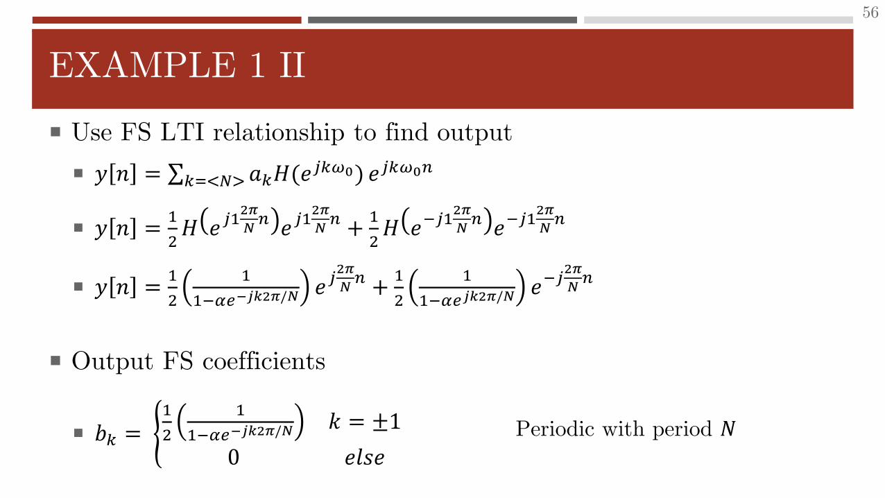
EXAMPLE 1 II
Use FS LTI relationship to find output
𝑦 𝑛 = σ𝑘=<𝑁> 𝑎𝑘𝐻(𝑒𝑗𝑘𝜔0) 𝑒𝑗𝑘𝜔0𝑛
𝑦 𝑛 =1
2𝐻 𝑒𝑗1
2𝜋
𝑁𝑛 𝑒𝑗1
2𝜋
𝑁𝑛 +
1
2𝐻 𝑒−𝑗1
2𝜋
𝑁𝑛 𝑒−𝑗1
2𝜋
𝑁𝑛
𝑦 𝑛 =1
2
1
1−𝛼𝑒−𝑗𝑘2𝜋/𝑁𝑒𝑗
2𝜋
𝑁𝑛 +
1
2
1
1−𝛼𝑒𝑗𝑘2𝜋/𝑁𝑒−𝑗
2𝜋
𝑁𝑛
Output FS coefficients
𝑏𝑘 = ൝1
2
1
1−𝛼𝑒−𝑗𝑘2𝜋/𝑁𝑘 = ±1
0 𝑒𝑙𝑠𝑒
56
Periodic with period 𝑁

𝑥(𝑡) has fundamental period 𝑇and FS 𝑎𝑘
Sometimes direct calculation of 𝑎𝑘 is difficult, at times easier to calculate transformation
𝑏𝑘 ↔ 𝑔 𝑡 =𝑑𝑥 𝑡
𝑑𝑡
Find 𝑎𝑘 in terms of 𝑏𝑘 and 𝑇, given
∫𝑇2𝑇𝑥 𝑡 𝑑𝑡 = 2
𝑎0 =1
𝑇∫𝑇 𝑥 𝑡 𝑒−𝑗 0 𝜔0𝑡𝑑𝑡 =
1
𝑇∫𝑇 𝑥 𝑡 𝑑𝑡 ⇒
2
𝑇
From Table 3.1 pg 206
𝑏𝑘 ↔ 𝑗𝑘2𝜋
𝑇𝑎𝑘 ⇒ 𝑎𝑘 =
𝑏𝑘
𝑗𝑘2𝜋/𝑇
𝑎𝑘 = ቐ2/𝑇 𝑘 = 0𝑏𝑘
𝑗𝑘2𝜋/𝑇𝑘 ≠ 0
57
EXAMPLE PROBLEM 3.7

EXAMPLE PROBLEM 3.7 II
Find FS of periodic sawtooth wave
Take derivative of sawtooth
Results in sum of rectangular waves
FS coefficients of rectangular waves from Table 3.2 to get 𝑏𝑘 ↔ 𝑔(𝑡)
Then use previous result to find 𝑎𝑘 ↔ 𝑥(𝑡)
See examples 3.6, 3.7 for similar treatment
58

CHAPTER 3.9FILTERING
59
FILTERING
Important process in many applications
The goal is to change the relative amplitudes of frequency components in a signal
In EE480: DSP you can learn how to design a filter with desired properties/specifications
60

LTI FILTERS
Frequency-shaping filters – general LTI systems
Frequency-selective filters – pass some frequencies and eliminate others
Common examples include low-pass (LP), high-pass (HP), bandpass (BP), and bandstop (BS) [notch]
61

MOTIVATION: AUDIO EQUALIZER
Basic equalizer gives user ability to adjust sound from to match taste – e.g. bass (low freq) and treble (high freq)
62
Log-log plot to show larger range of frequencies and response
dB = 20 log10 𝐻 𝑗𝜔
Magnitude response matches are intuition Boost low and high frequencies
but attenuate mid frequencies

EXAMPLE: DERIVATIVE FILTER
𝑦 𝑡 =𝑑
𝑑𝑡𝑥 𝑡 ⟷ 𝐻 𝑗𝜔 = 𝑗𝜔
High-pass filter used for “edge” detection
63

EXAMPLE: AVERAGE FILTER
𝑦 𝑛 =1
2𝑥 𝑛 + 𝑥 𝑛 − 1
Low-pass filter used for smoothing
64

MATLAB FOR FILTERS
Very helpful to visualize filters
65

Continuous Case
𝑥 𝑡 = σ𝑘 𝑎𝑘𝑒𝑗𝑘𝜔0𝑡
𝑎𝑘 =1
𝑇∫𝑇 𝑥 𝑡 𝑒−𝑗𝑘𝜔0𝑡𝑑𝑡
Fundamental frequency 𝜔0
Fundamental period 𝑇 =2𝜋
𝜔0
Discrete Case
𝑥[𝑛] = σ𝑘=<𝑁>𝑎𝑘𝑒𝑗𝑘𝜔0𝑛
𝑎𝑘 =1
𝑁σ𝑛=<𝑁> 𝑥 𝑛 𝑒−𝑗𝑘𝜔0𝑛
Fundamental frequency 𝜔0
Fundamental period 𝑁 =2𝜋
𝜔0
66
FOURIER SERIES SUMMARY


