EEL 6266 Power System Operation and Control
Chapter 5
Unit Commitment

© 2002, 2004 Florida State University EEL 6266 Power System Operation and Control 2
Unit Commitment Solution Methods
� Dynamic programming� chief advantage over enumeration schemes is the reduction in
the dimensionality of the problem� in a strict priority order scheme, there are only N combinations
to try for an N unit system
� a strict priority list would result in a theoretically correct dispatch and commitment only if� the no-load costs are zero
� unit input-output characteristics are linear
� there are no other limits, constraints, or restrictions
� start-up costs are a fixed amount
© 2002, 2004 Florida State University EEL 6266 Power System Operation and Control 3
Unit Commitment Solution Methods
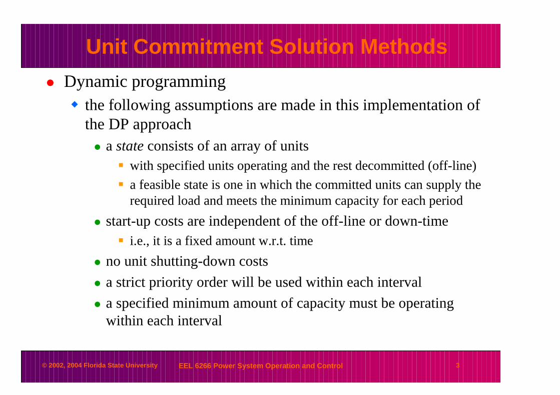
� Dynamic programming� the following assumptions are made in this implementation of
the DP approach� a stateconsists of an array of units
� with specified units operating and the rest decommitted (off-line)
� a feasible state is one in which the committed units can supply the required load and meets the minimum capacity for each period
� start-up costs are independent of the off-line or down-time� i.e., it is a fixed amount w.r.t. time
� no unit shutting-down costs
� a strict priority order will be used within each interval
� a specified minimum amount of capacity must be operating within each interval
© 2002, 2004 Florida State University EEL 6266 Power System Operation and Control 4
Unit Commitment Solution Methods
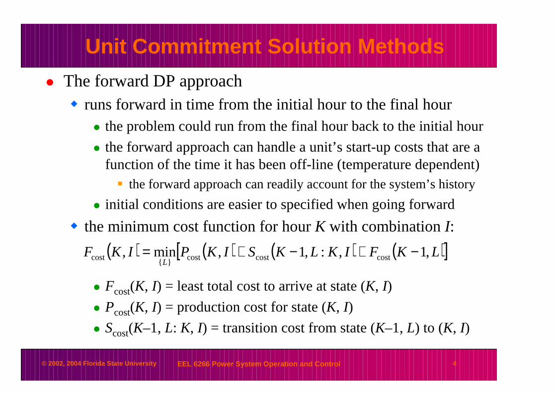
� The forward DP approach� runs forward in time from the initial hour to the final hour
� the problem could run from the final hour back to the initial hour
� the forward approach can handle a unit’s start-up costs that are a function of the time it has been off-line (temperature dependent)� the forward approach can readily account for the system’s history
� initial conditions are easier to specified when going forward
� the minimum cost function for hour K with combination I:
� Fcost(K, I) = least total cost to arrive at state (K, I)
� Pcost(K, I) = production cost for state (K, I)
� Scost(K–1, L: K, I) = transition cost from state (K–1, L) to (K, I)
( ) ( ) ( ) ( )[ ]LKFIKLKSIKPIKFL
,1,:,1,min, costcostcost}{
cost −+−+=
© 2002, 2004 Florida State University EEL 6266 Power System Operation and Control 5
Unit Commitment Solution Methods
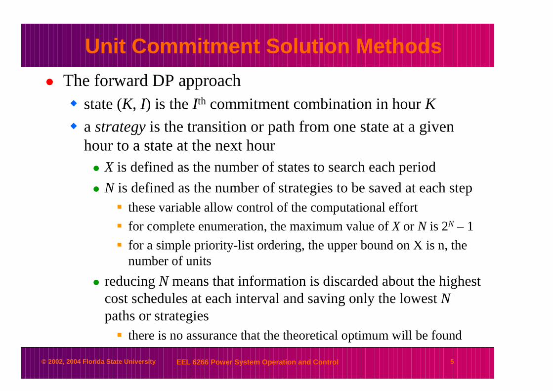
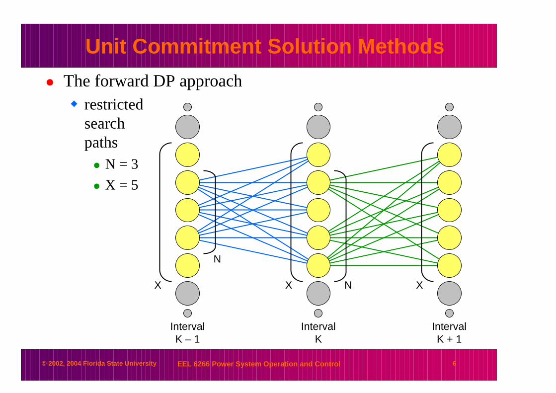
� The forward DP approach� state (K, I) is the I th commitment combination in hour K
� a strategyis the transition or path from one state at a given hour to a state at the next hour� X is defined as the number of states to search each period
� N is defined as the number of strategies to be saved at each step� these variable allow control of the computational effort
� for complete enumeration, the maximum value of X or N is 2N – 1
� for a simple priority-list ordering, the upper bound on X is n, the number of units
� reducing N means that information is discarded about the highest cost schedules at each interval and saving only the lowest Npaths or strategies� there is no assurance that the theoretical optimum will be found
© 2002, 2004 Florida State University EEL 6266 Power System Operation and Control 6
Unit Commitment Solution Methods
� The forward DP approach� restricted
searchpaths� N = 3
� X = 5
IntervalK – 1
IntervalK
IntervalK + 1
X X X
N
N

© 2002, 2004 Florida State University EEL 6266 Power System Operation and Control 7
Unit Commitment Solution Methods
� Example� consider a system with 4 units to serve an 8 hour load pattern
Incremental No-load Full-load Min. TimeUnit Pmax Pmin Heat Rate Cost Ave. Cost (h)
(MW) (MW) (Btu / kWh) ($ / h) ($ / mWh) Up Down
1 80 25 10440 213.00 23.54 4 22 250 60 9000 585.62 20.34 5 33 300 75 8730 684.74 19.74 5 44 60 20 11900 252.00 28.00 1 1
Initial Condition Start-up CostsUnit off(-) / on(+) Hot Cold Cold start
(h) ($) ($) (h)
1 -5 150 350 42 8 170 400 53 8 500 1100 54 -6 0 0.02 0
Hour Load (MW)
1 4502 5303 6004 5405 4006 2807 2908 500
© 2002, 2004 Florida State University EEL 6266 Power System Operation and Control 8
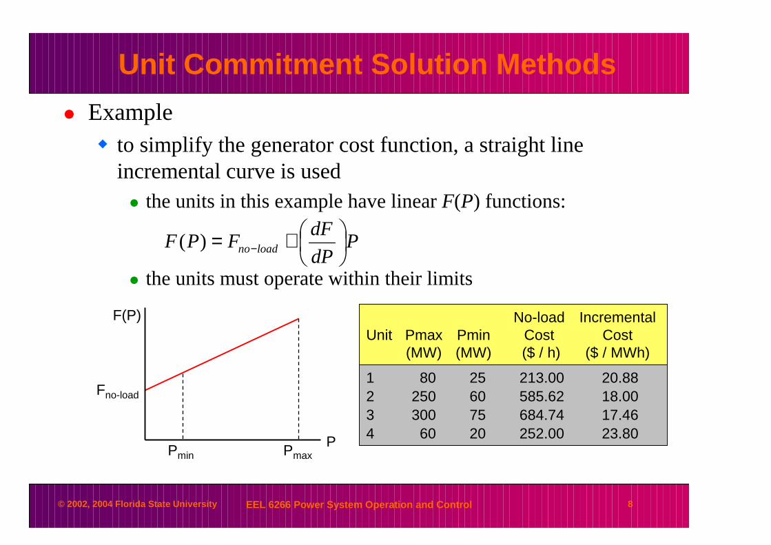
Unit Commitment Solution Methods
� Example� to simplify the generator cost function, a straight line
incremental curve is used� the units in this example have linear F(P) functions:
� the units must operate within their limits
PdP
dFFPF loadno
+= −)(
F(P)
Fno-load
Pmin PmaxP
No-load IncrementalUnit Pmax Pmin Cost Cost
(MW) (MW) ($ / h) ($ / MWh)
1 80 25 213.00 20.882 250 60 585.62 18.003 300 75 684.74 17.464 60 20 252.00 23.80

© 2002, 2004 Florida State University EEL 6266 Power System Operation and Control 9
Unit Commitment Solution Methods
� Case 1: Strict priority-list ordering� the only states examined each hour
consist of the listed four:� state 5: unit 3, state 12: 3 + 2
state 14: 3 + 2 + 1, state 15: all four
� all possible commitments start from state 12 (initial condition)
� minimum unit up and down times are ignored
� in hour 1:� possible states that meet load demand (450 MW): 12, 14, & 15
State Unit status Capacity
5 0 0 1 0 300 MW12 0 1 1 0 550 MW14 1 1 1 0 630 MW15 1 1 1 1 690 MW
( ) ( ) ( ) ( ) ( )( ) ( ) ( ) ( )
( ) ( ) ( )( ) ( ) ( )[ ] 38.1021102.035036.9861
15,1:12,015,115,1
36.98612080.2330046.1710500.182588.2036.1735
203001052515,1
costcostcost
1321cost
=++=+=
=++++=+++=
SPF
FFFFP Economic Dispatch Eq.
DP State Transition Eq.
© 2002, 2004 Florida State University EEL 6266 Power System Operation and Control 10
Unit Commitment Solution Methods
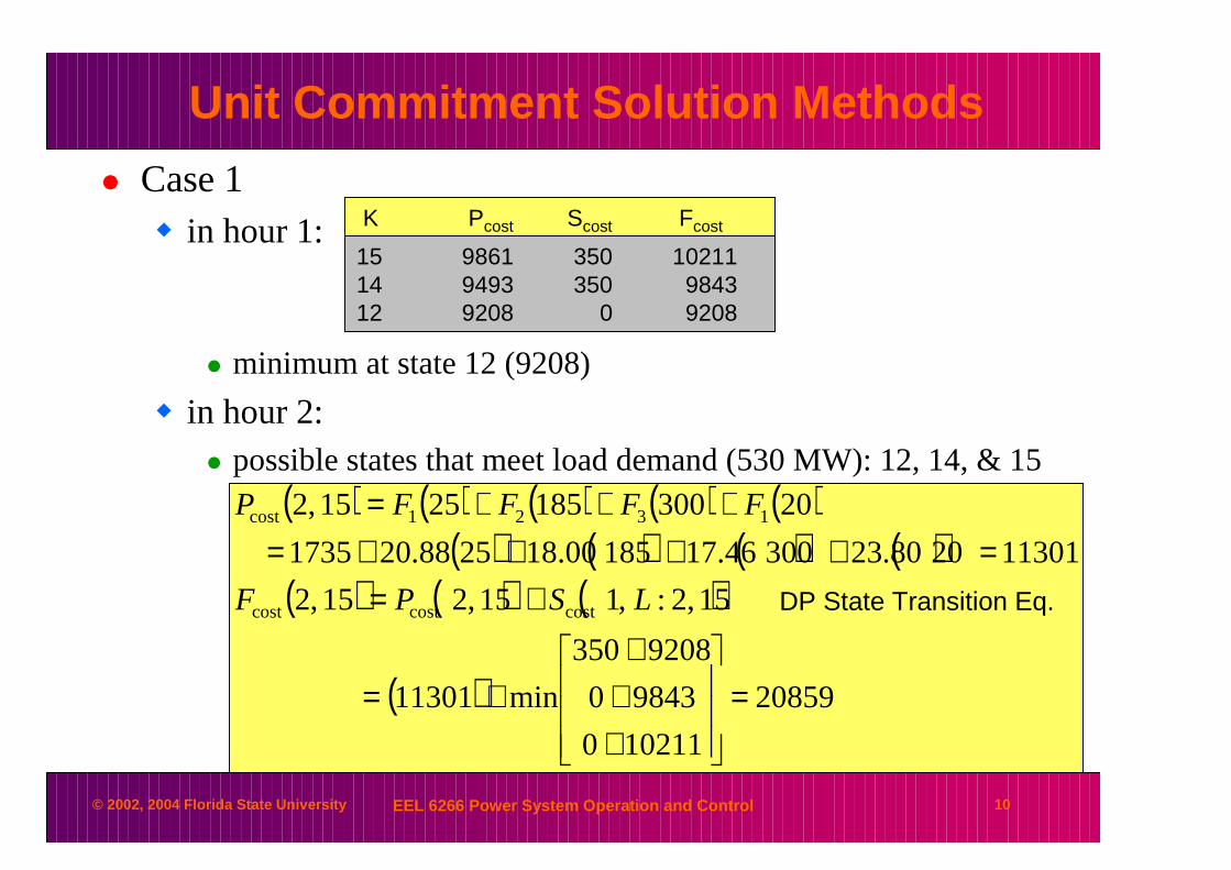
� Case 1� in hour 1:
� minimum at state 12 (9208)
� in hour 2:� possible states that meet load demand (530 MW): 12, 14, & 15
K Pcost Scost Fcost
15 9861 350 1021114 9493 350 984312 9208 0 9208
( ) ( ) ( ) ( ) ( )( ) ( ) ( ) ( )
( ) ( ) ( )
( ) 20859
102110
98430
9208350
min11301
15,2:,115,215,2
113012080.2330046.1718500.182588.201735
203001852515,2
costcostcost
1321cost
=
+++
+=
+==++++=
+++=
LSPF
FFFFP
DP State Transition Eq.
© 2002, 2004 Florida State University EEL 6266 Power System Operation and Control 11
Unit Commitment Solution Methods
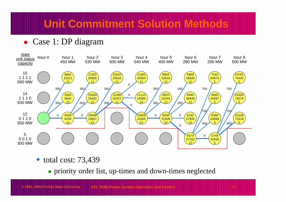
� Case 1: DP diagram
� total cost: 73,439� priority order list, up-times and down-times neglected
151 1 1 1
690 MW
141 1 1 0
630 MW
120 1 1 0
550 MW
50 0 1 0
300 MW
stateunit statuscapacity
hour 1450 MW
hour 2530 MW
hour 3600 MW
hour 4540 MW
hour 5400 MW
hour 6280 MW
hour 7290 MW
hour 8500 MW
hour 0
986110211
12
94939843
12
92089208
12
1130120860
12
1093320492
12
1064819857
12
1341033618
12
1226532472
12
557457182
12
1148143953
14
1111343585
14
1082843300
14
896452615
12
859352244
12
830851609
12
686958828
12
649058449
12
619257800
12
704364976
5
666564597
5
636663949
5
1076174442
5
1039374074
5
1010873439
5
574862930
5
350 350 350 350 350
350 350 350
0
350 350
0
0 0
0
0 0
0
750
750
400
0
750
750
400
© 2002, 2004 Florida State University EEL 6266 Power System Operation and Control 12
Unit Commitment Solution Methods
� Case 2:� complete enumeration (2.56 × 10⁹ possibilities)
� fortunately, most are not feasible because they do not supply sufficient capacity
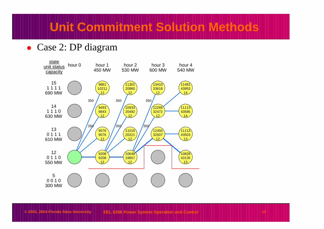
� in this case, the true optimal commitment is found� the only difference in the two trajectories occurs in hour 3
� it is less expensive to turn on the less efficient peaking unit #4 for three hours than to start up the more efficient unit #1 for that same time period
� only minor improvement to the total cost� case 1: 73,439
� case 2: 73,274
© 2002, 2004 Florida State University EEL 6266 Power System Operation and Control 13
Unit Commitment Solution Methods
� Case 2: DP diagram
151 1 1 1
690 MW
141 1 1 0
630 MW
120 1 1 0
550 MW
50 0 1 0
300 MW
stateunit statuscapacity
hour 1450 MW
hour 2530 MW
hour 3600 MW
hour 4540 MW
hour 0
986110211
12
94939843
12
92089208
12
1130120860
12
1093320492
12
1064819857
12
1341033618
12
1226532472
12
1148143953
14
1111343585
14
1082843135
13
350 350
350 35013
0 1 1 1610 MW
95769576
12
1101620221
12
1245032507
12
1111343503
13
350
350
© 2002, 2004 Florida State University EEL 6266 Power System Operation and Control 14
Unit Commitment Solution Methods
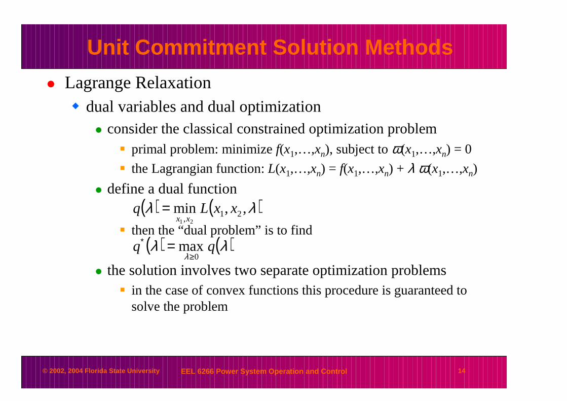
� Lagrange Relaxation� dual variables and dual optimization
� consider the classical constrained optimization problem� primal problem: minimize f(x1,…,xn), subject to ω(x1,…,xn) = 0
� the Lagrangian function: L(x1,…,xn) = f(x1,…,xn) + λ ω(x1,…,xn)
� define a dual function
� then the “dual problem” is to find
� the solution involves two separate optimization problems� in the case of convex functions this procedure is guaranteed to
solve the problem
( ) ( )λλλ
qq0
max≥
∗ =
( ) ( )λλ ,,min 21, 21
xxLqxx
=
© 2002, 2004 Florida State University EEL 6266 Power System Operation and Control 15
Unit Commitment Solution Methods
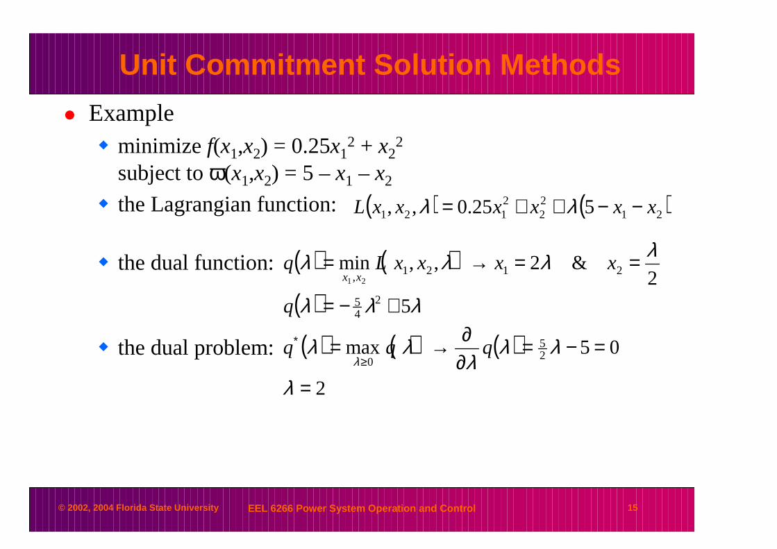
� Example� minimize f(x1,x2) = 0.25x1
2 + x22
subject to ω(x1,x2) = 5 –x1 – x2
� the Lagrangian function:
� the dual function:
� the dual problem: ( ) ( ) ( )2
05max 25
0
=
=−=∂∂→=
≥
∗
λ
λλλ
λλλ
qqq
( ) ( )
( ) λλλ
λλλλ
52
&2,,min
245
2121, 21
+−=
==→=
q
xxxxLqxx
( ) ( )2122
2121 525.0,, xxxxxxL −−++= λλ
© 2002, 2004 Florida State University EEL 6266 Power System Operation and Control 16
Unit Commitment Solution Methods
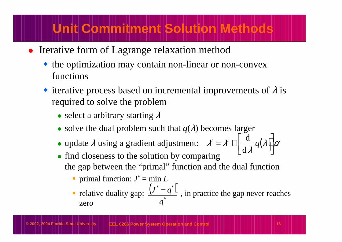
� Iterative form of Lagrange relaxation method� the optimization may contain non-linear or non-convex
functions
� iterative process based on incremental improvements of λ is required to solve the problem� select a arbitrary starting λ� solve the dual problem such that q(λ) becomes larger
� update λ using a gradient adjustment:
� find closeness to the solution by comparing the gap between the “primal” function and the dual function� primal function: J* = min L
� relative duality gap: , in practice the gap never reaches zero
( ) αλλ
λλ
+= qtt
d
d
( )*
**
q
qJ −
© 2002, 2004 Florida State University EEL 6266 Power System Operation and Control 17
Unit Commitment Solution Methods
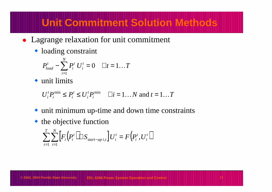
� Lagrange relaxation for unit commitment� loading constraint
� unit limits
� unit minimum up-time and down time constraints
� the objective function
TtUPPN
i
ti
ti
tload K10
1
=∀=−∑=
TtNiPUPPU iti
tii
ti KK 1 and 1minmin ==∀≤≤
( )[ ] ( )ti
ti
T
t
N
i
titiupstart
tii UPFUSPF ,
1 1, =+∑∑
= =−
© 2002, 2004 Florida State University EEL 6266 Power System Operation and Control 18
Unit Commitment Solution Methods
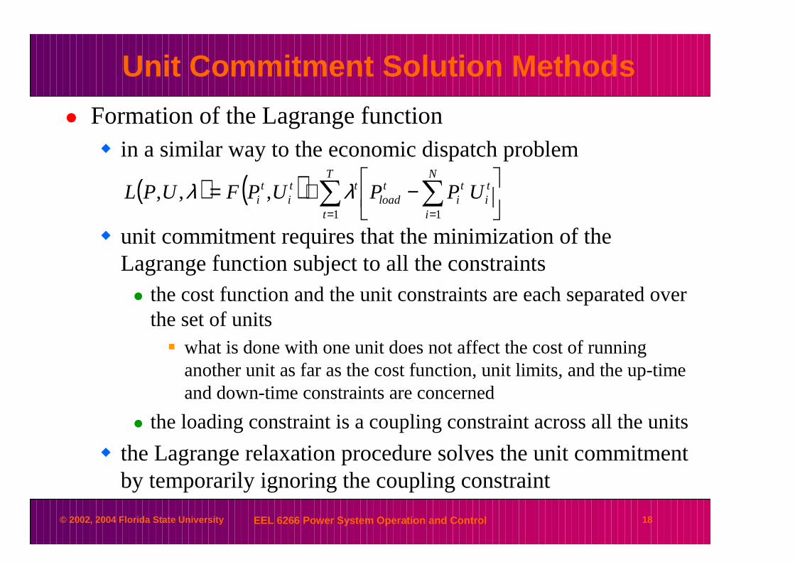
� Formation of the Lagrange function� in a similar way to the economic dispatch problem
� unit commitment requires that the minimization of the Lagrange function subject to all the constraints� the cost function and the unit constraints are each separated over
the set of units� what is done with one unit does not affect the cost of running
another unit as far as the cost function, unit limits, and the up-time and down-time constraints are concerned
� the loading constraint is a coupling constraint across all the units
� the Lagrange relaxation procedure solves the unit commitment by temporarily ignoring the coupling constraint
( ) ( ) ∑ ∑= =
−+=T
t
N
i
ti
ti
tload
tti
ti UPPUPFUPL
1 1
,,, λλ
© 2002, 2004 Florida State University EEL 6266 Power System Operation and Control 19
Unit Commitment Solution Methods
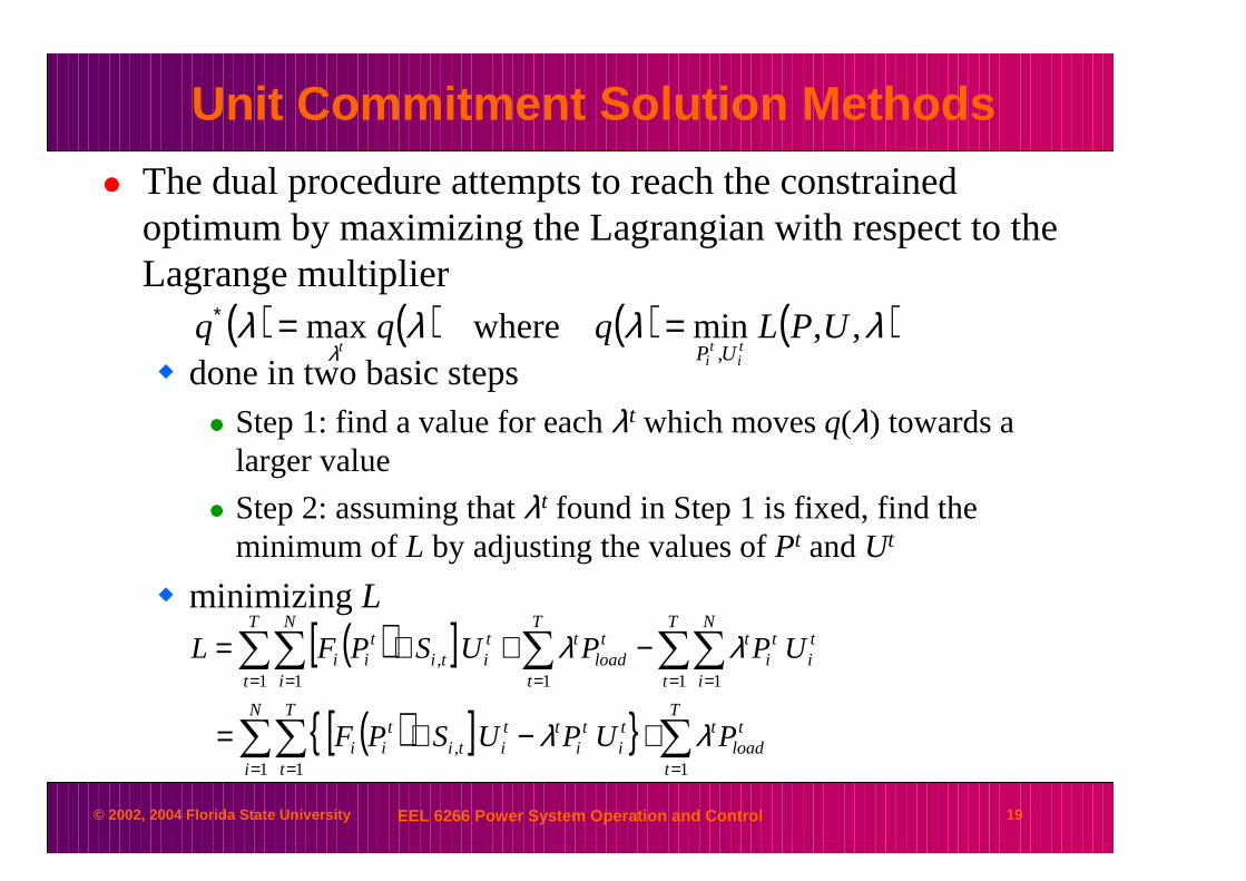
� The dual procedure attempts to reach the constrained optimum by maximizing the Lagrangian with respect to the Lagrange multiplier
� done in two basic steps� Step 1: find a value for each λt which moves q(λ) towards a
larger value
� Step 2: assuming that λt found in Step 1 is fixed, find the minimum of L by adjusting the values of Pt and Ut
� minimizing L
( ) ( ) ( ) ( )λλλλλ
,,minwheremax,
UPLqqqti
ti
t UP==∗
( )[ ]
( )[ ]{ } ∑∑∑
∑∑∑∑∑
== =
= === =
+−+=
−++=
T
t
tload
tN
i
T
t
ti
ti
ttiti
tii
T
t
N
i
ti
ti
tT
t
tload
tT
t
N
i
titi
tii
PUPUSPF
UPPUSPFL
11 1,
1 111 1,
λλ
λλ
© 2002, 2004 Florida State University EEL 6266 Power System Operation and Control 20
Unit Commitment Solution Methods
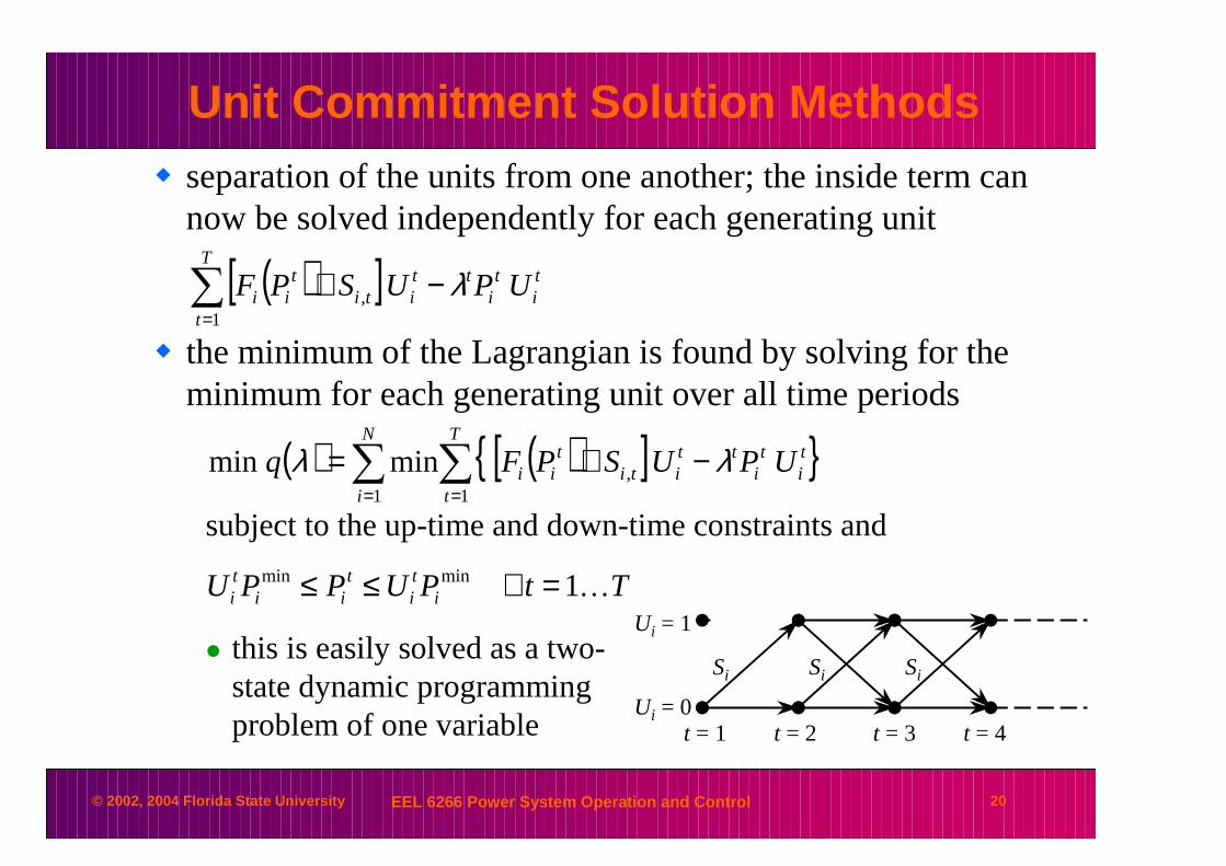
� separation of the units from one another; the inside term can now be solved independently for each generating unit
� the minimum of the Lagrangian is found by solving for the minimum for each generating unit over all time periods
subject to the up-time and down-time constraints and
� this is easily solved as a two-state dynamic programming problem of one variable
( )[ ]∑=
−+T
t
ti
ti
ttiti
tii UPUSPF
1, λ
( ) ( )[ ]{ }∑∑==
−+=T
t
ti
ti
ttiti
tii
N
i
UPUSPFq1
,1
minmin λλ
TtPUPPU iti
tii
ti K1minmin =∀≤≤
Ui = 1
Ui = 0t = 1 t = 2 t = 3 t = 4
Si Si Si
© 2002, 2004 Florida State University EEL 6266 Power System Operation and Control 21
Unit Commitment Solution Methods
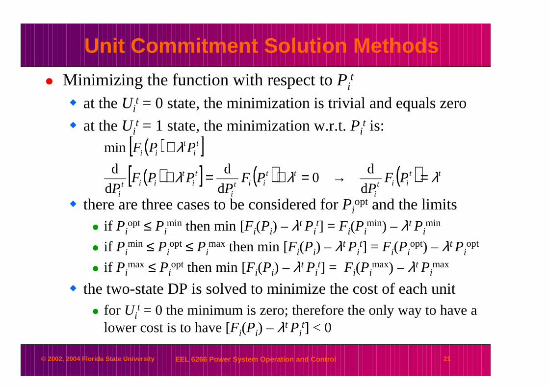
� Minimizing the function with respect to Pit
� at the Uit = 0 state, the minimization is trivial and equals zero
� at the Uit = 1 state, the minimization w.r.t. Pi
t is:
� there are three cases to be considered for Piopt and the limits
� if Piopt ≤ Pi
min then min [Fi(Pi) – λt Pit] = Fi(Pi
min) – λt Pimin
� if Pimin ≤ Pi
opt ≤ Pimax then min [Fi(Pi) – λt Pi
t] = Fi(Piopt) – λt Pi
opt
� if Pimax ≤ Pi
opt then min [Fi(Pi) – λt Pit] = Fi(Pi
max) – λt Pimax
� the two-state DP is solved to minimize the cost of each unit� for Ui
t = 0 the minimum is zero; therefore the only way to have a lower cost is to have [Fi(Pi) – λt Pi
t] < 0
( )[ ]( )[ ] ( ) ( ) tt
iiti
ttiit
i
ti
tiit
i
ti
tii
PFP
PFP
PPFP
PPF
λλλ
λ
=→=+=+
+
d
d0
d
d
d
d
min
© 2002, 2004 Florida State University EEL 6266 Power System Operation and Control 22
Unit Commitment Solution Methods
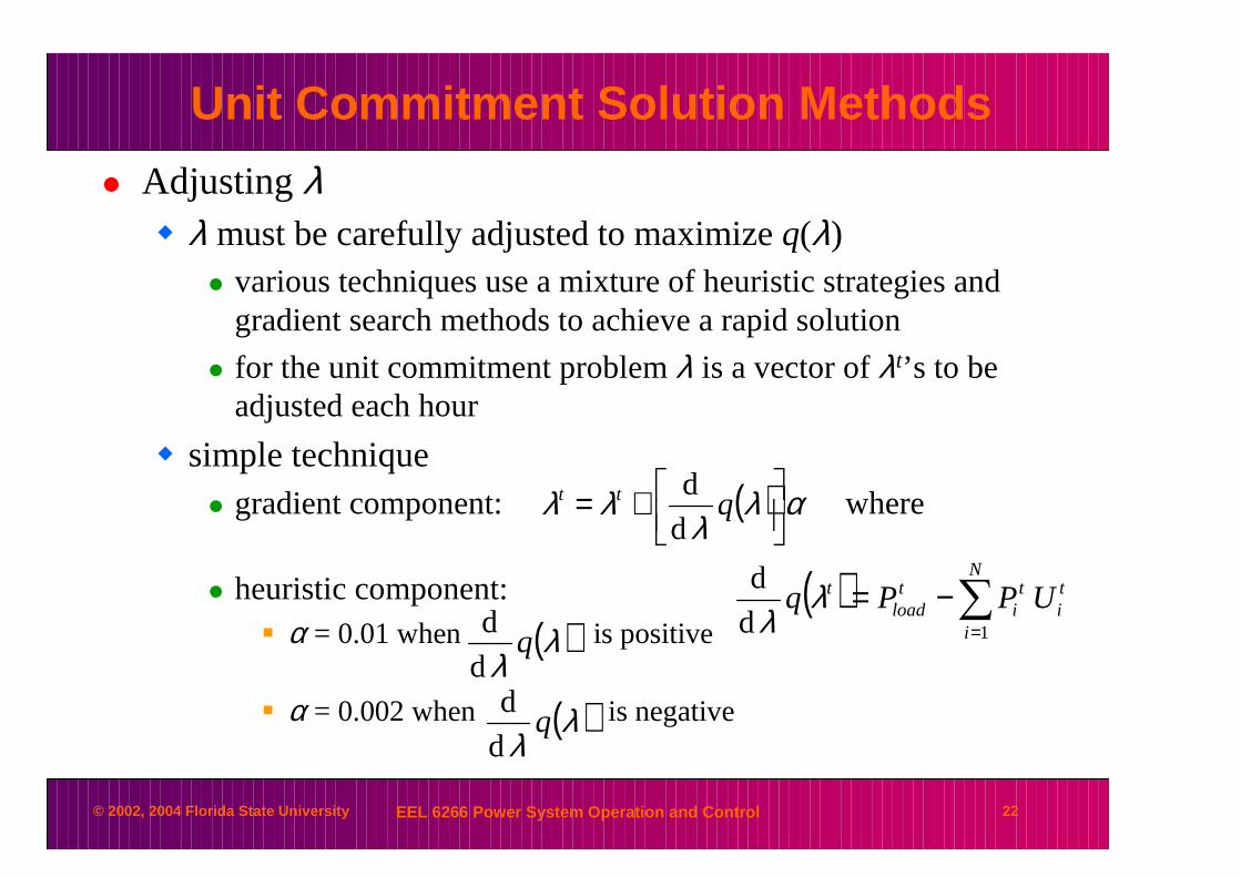
� Adjusting λ� λ must be carefully adjusted to maximize q(λ)
� various techniques use a mixture of heuristic strategies and gradient search methods to achieve a rapid solution
� for the unit commitment problem λ is a vector of λt’s to be adjusted each hour
� simple technique� gradient component: where
� heuristic component:� α = 0.01 when is positive
� α = 0.002 when is negative
( )
( ) ∑=
−=
+=
N
i
ti
ti
tload
t
tt
UPPq
q
1d
d
d
d
λλ
αλλ
λλ
( )λλ
qdd
( )λλ
qdd
© 2002, 2004 Florida State University EEL 6266 Power System Operation and Control 23
Unit Commitment Solution Methods
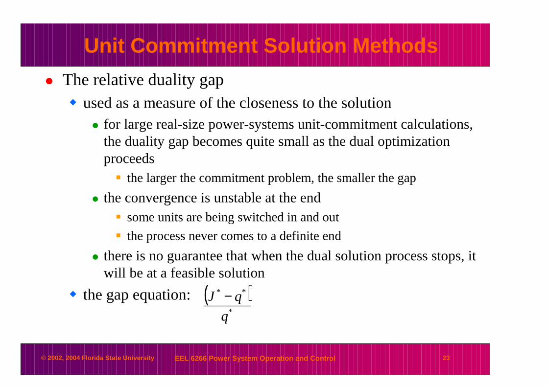
� The relative duality gap� used as a measure of the closeness to the solution
� for large real-size power-systems unit-commitment calculations, the duality gap becomes quite small as the dual optimization proceeds� the larger the commitment problem, the smaller the gap
� the convergence is unstable at the end� some units are being switched in and out
� the process never comes to a definite end
� there is no guarantee that when the dual solution process stops, it will be at a feasible solution
� the gap equation:( )*
**
q
qJ −
© 2002, 2004 Florida State University EEL 6266 Power System Operation and Control 24
Unit Commitment Solution Methods
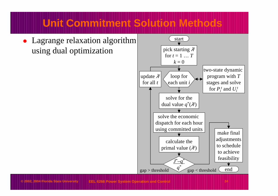
� Lagrange relaxation algorithm using dual optimization
start
pick starting λt
for t = 1 … Tk = 0
J*–q*
q*
loop foreach unit i
two-state dynamic program with Tstages and solvefor Pi
t and Uit
solve for thedual value q*(λt)
solve the economic dispatch for each hourusing committed units
calculate theprimal value (λt)
update λt
for all t
end
make finaladjustmentsto scheduleto achievefeasibility
gap < thresholdgap > threshold
© 2002, 2004 Florida State University EEL 6266 Power System Operation and Control 25
Unit Commitment Solution Methods
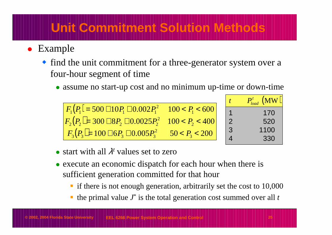
� Example� find the unit commitment for a three-generator system over a
four-hour segment of time� assume no start-up cost and no minimum up-time or down-time
� start with all λt values set to zero
� execute an economic dispatch for each hour when there is sufficient generation committed for that hour� if there is not enough generation, arbitrarily set the cost to 10,000
� the primal value J* is the total generation cost summed over all t
( )( )( ) 20050005.06100
4001000025.08300
600100002.010500
32
3333
22
2222
12
1111
<<++=<<++=<<++=
PPPPF
PPPPF
PPPPF( )MWt
loadPt
1 1702 520 3 11004 330
© 2002, 2004 Florida State University EEL 6266 Power System Operation and Control 26
Unit Commitment Solution Methods
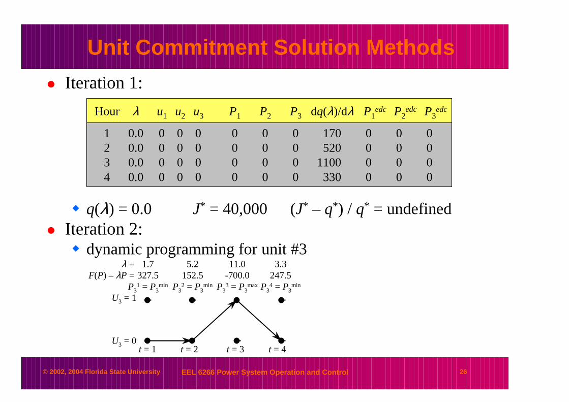
� Iteration 1:
� q(λ) = 0.0 J* = 40,000 (J* – q*) / q* = undefined� Iteration 2:
� dynamic programming for unit #3
Hour λ u1 u2 u3 P1 P2 P3 dq(λ)/dλ P1edc P2
edc P3edc
1 0.0 0 0 0 0 0 0 170 0 0 02 0.0 0 0 0 0 0 0 520 0 0 03 0.0 0 0 0 0 0 0 1100 0 0 04 0.0 0 0 0 0 0 0 330 0 0 0
U3 = 1
U3 = 0t = 1 t = 2 t = 3 t = 4
3.3247.5
P34 = P3
min
11.0-700.0
P33 = P3
max
5.2152.5
P32 = P3
min
1.7327.5
P31 = P3
min
λ =F(P) – λP =
© 2002, 2004 Florida State University EEL 6266 Power System Operation and Control 27
Unit Commitment Solution Methods
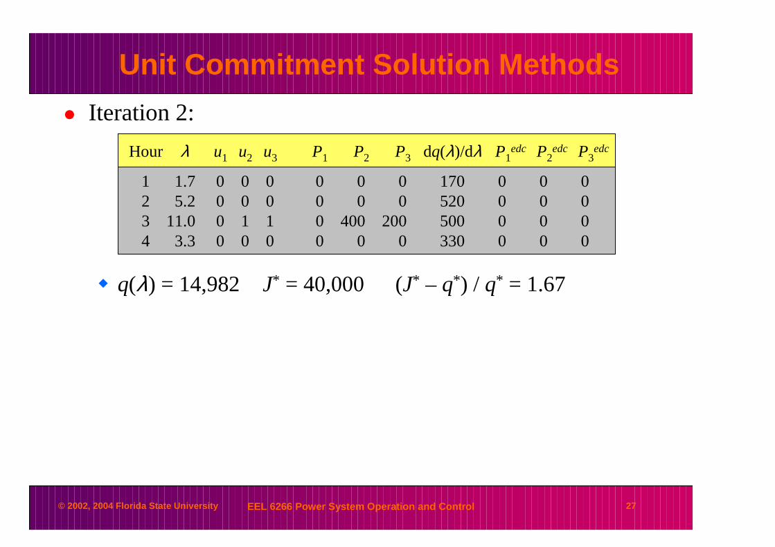
� Iteration 2:
� q(λ) = 14,982 J* = 40,000 (J* – q*) / q* = 1.67
Hour λ u1 u2 u3 P1 P2 P3 dq(λ)/dλ P1edc P2
edc P3edc
1 1.7 0 0 0 0 0 0 170 0 0 02 5.2 0 0 0 0 0 0 520 0 0 03 11.0 0 1 1 0 400 200 500 0 0 04 3.3 0 0 0 0 0 0 330 0 0 0

© 2002, 2004 Florida State University EEL 6266 Power System Operation and Control 28
Unit Commitment Solution Methods
� Iteration 3:
� q(λ) = 18,344 J* = 36,024 (J* – q*) / q* = 0.965
Hour λ u1 u2 u3 P1 P2 P3 dq(λ)/dλ P1edc P2
edc P3edc
1 3.4 0 0 0 0 0 0 170 0 0 02 10.4 0 1 1 0 400 200 -80 0 320 2003 16.0 1 1 1 600 400 200 -100 500 400 2004 6.6 0 0 0 0 0 0 330 0 0 0

© 2002, 2004 Florida State University EEL 6266 Power System Operation and Control 29
Unit Commitment Solution Methods
� Iteration 4:
� q(λ) = 19,214 J* = 28,906 (J* – q*) / q* = 0.502
Hour λ u1 u2 u3 P1 P2 P3 dq(λ)/dλ P1edc P2
edc P3edc
1 5.1 0 0 0 0 0 0 170 0 0 02 10.24 0 1 1 0 400 200 -80 0 320 2003 15.8 1 1 1 600 400 200 -100 500 400 2004 9.9 0 1 1 0 380 200 -250 0 130 200
© 2002, 2004 Florida State University EEL 6266 Power System Operation and Control 30
Unit Commitment Solution Methods
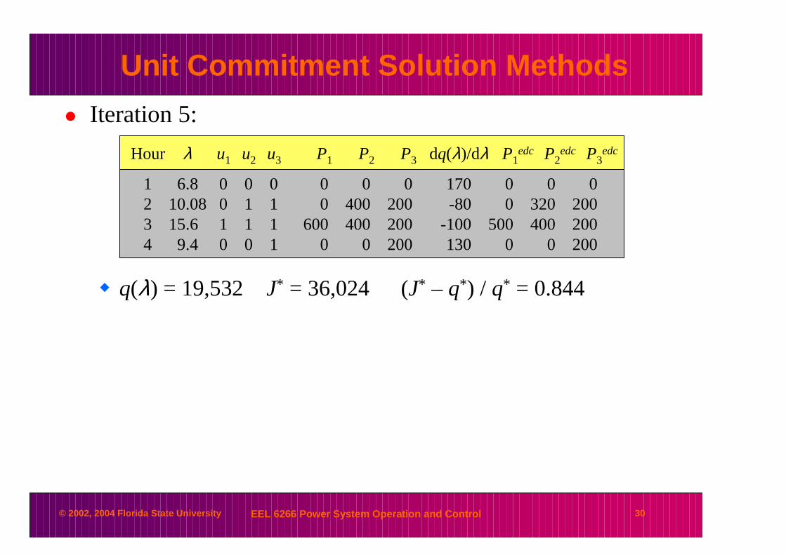
� Iteration 5:
� q(λ) = 19,532 J* = 36,024 (J* – q*) / q* = 0.844
Hour λ u1 u2 u3 P1 P2 P3 dq(λ)/dλ P1edc P2
edc P3edc
1 6.8 0 0 0 0 0 0 170 0 0 02 10.08 0 1 1 0 400 200 -80 0 320 2003 15.6 1 1 1 600 400 200 -100 500 400 2004 9.4 0 0 1 0 0 200 130 0 0 200

© 2002, 2004 Florida State University EEL 6266 Power System Operation and Control 31
Unit Commitment Solution Methods
� Iteration 6:
� q(λ) = 19,442 J* = 20,170 (J* – q*) / q* = 0.037� Remarks
� the commitment schedule does not change significantly with further iterations� however, the solution is not stable (oscillation of unit 2)
� the duality gap does reduce� after 10 iterations, the gap reduces to 0.027� good stopping criteria would be when the gap reaches 0.05
Hour λ u1 u2 u3 P1 P2 P3 dq(λ)/dλ P1edc P2
edc P3edc
1 8.5 0 0 1 0 0 200 -30 0 0 1702 9.92 0 1 1 0 384 200 -64 0 320 2003 15.4 1 1 1 600 400 200 -100 500 400 2004 10.7 0 1 1 0 400 200 -270 0 130 200


