1
Efficient Reversible Data Hiding Based on the Use of Multiple Predictors
Abstract
Reversible data hiding (RDH) algorithms are concerned with the recovery of the original cover image
upon the extraction of the digital signature or watermark. In some RDH algorithms, embedding and
extraction are performed through modifying the histogram of prediction errors that are computed using
some predictor. However, the embedding capacity and image quality in these algorithms are dependent on
the characteristics of a single predictor and its ability to produce accurate predictions. In this paper, we
propose the idea of employing multiple predictors in order to increase the embedding capacity. The idea
of multiple predictors is integrated in the modification of the prediction errors (MPE) algorithm without
adding any overhead regarding the predictor that is used for embedding at each pixel in the image. The
selection criterion of the accurate predictor uses the minimum, median or maximum of prediction errors
based on their polarity. Experimental results proved the efficiency of the proposed algorithm when
compared to the MPE algorithm and its variations.
Keywords: Prediction, prediction error, histogram shifting, reversible data hiding.
1. Introduction
Proving the authenticity and ownership of digital images has become an issue recently due to the
wide spread of digital devices and the ease of manipulation of digital multimedia. One way around this
issue is the use of digital image watermarking or data hiding [1]. In this approach, digital signatures or
watermarks are seamlessly embedded in a digital image (the cover image) to facilitate authentication and
verification purposes. Several watermarking or data hiding algorithms have been proposed in the
literature. Some of these algorithms are implemented in the spatial domain [2-4] while others are
transform-based algorithms [5]. The key differences between different algorithms lie in the capability of
embedding large payloads, transparency of the watermark, the quality of the watermarked or stego image

2
and the complexity. However, most of these watermarking algorithms are irreversible in the sense that the
original image cannot be recovered once the digital signature or watermark is extracted. Such requirement
is very important when it comes to sensitive imaging applications related to medical and military images.
Accordingly, a new class of data hiding algorithms has emerged. These algorithms are usually
referred to as reversible data hiding (RDH) algorithms and are capable of restoring the original cover
image. Despite the fact that such requirement may result in lower payloads, higher computational costs,
and larger distortion in the watermarked image, many algorithms were proposed in the literature to meet
the reversibility requirement in some applications. Originally, RDH algorithms relied on lossless
compression [6], [7]. In such algorithms, such as the least significant bit (LSB) of the pixels, a portion of
the image is losslessly compressed and saved in order to open space to embed the signature. Despite of
their simplicity, the embedding capacity of such algorithms is relatively low. The concept of difference
expansion in reversible data hiding was proposed in [8]. The technique uses a decorrelation operator
between pixel pairs in the image to create features with small magnitudes. The digital watermark is
inserted in an expanded version of these features. Several approaches were built on the difference
expansion technique [9], [10]. However, algorithms based on difference expansion suffered from
undesirable distortion in the stego image when the values of the used features are large.
A different strategy for hiding data reversibly in digital images and that is capable of reducing the
distortion was proposed by Ni et al. [11]. Commonly, this technique and similar ones are referred to as
histogram shifting or histogram modification techniques. The basic idea in the original histogram shifting
algorithm is to empty one or more of the bins in the image histogram through shifting of pixels’ values in
order to open space for the secret message to be embedded. This is performed by searching for a peak and
zero (or minimum) bins in the image histogram and then shifting all bins that lie between a pair of peak
and zero by one bin. Next, the bits of the secret message are inserted either in the pixels with gray level
value of the peak or in the value that is next to the peak which was made vacant through shifting. This
technique requires saving the pair(s) of peak and zero points in addition to the pixels that may result in
overflow and underflow as an overhead in order to ensure reversibility. The performance of this technique
3
guaranteed the quality of the watermarked or stego image to be higher than 48.13 dB. Nonetheless, the
embedding capacity of the algorithm is dependent on the height and number of peak(s) in the gray level
distribution of the image histogram, which are relatively of low counts in natural images.
Due to the simplicity and efficiency of Ni’s algorithm, several approaches exploited the use of
histogram shifting in reversible data hiding for the purpose of increasing the embedding. Fallahpour and
Sedaaghi [12] proposed applying the histogram shifting to image blocks instead of the entire image. In
[13] histogram shifting was applied to pixel differences which were obtained from the absolute
differences between pairs of pixels in the cover image. These extensions on the histogram shifting
technique showed significant improvement in terms of embedding capacity.
An interesting extension to reversible data hiding using the histogram shifting approach relied on the
concept of prediction. Hong et al. [14] proposed embedding the secret data by modifying the histogram of
prediction errors instead of intensity histogram of the image. The rationale behind using the prediction
errors is that the values of these errors are sharply centered near the origin due to the spatial correlation
between neighboring pixels in the image. This implies that the highest peak in the prediction error
histograms will have higher values than the peak(s) in the image intensity histogram. In this technique,
the median edge detector (MED) is used to compute the predicted pixel value. In order to embed data,
some values of the prediction errors are modified to embed the bits of the secret message. Specifically,
prediction errors with values 0 and -1 are used for embedding the data. On other hand, prediction errors
greater than 1 and less than -1 are incremented and decremented by 1, respectively. This is done to open
vacant bins at 1 and -2 to allow embedding of secret bits with value of 1, while zero bits are embedded in
the 0 and -1 bins. This algorithm showed impressive results in terms of boosting the embedding capacity.
Additionally, and similar to [11] the quality of the stego image is guaranteed to have a lower bound of
48.13 dB since all bins the prediction error histogram are shifted by 1 in the worst case. Actually, the
embedding capacity of the MPE algorithm can be increased further by using more bins in the prediction
error histogram. However, this violates the lower bound of the image quality as using more bins requires
for embedding requires emptying more bins through shifting of the histogram bins.

4
Many algorithms utilized the idea of prediction for reversible data embedding. The main difference
among such algorithms is basically related to the type of the used predictor and the way the prediction
errors are modified [15]. For example, the algorithm in [16] is basically the algorithm of Hong et al. that
utilizes a new fuzzy predictor in computing the predictions. The algorithm in [17] relied on checkerboard
pattern and the least-square method to improve the prediction performance for the sake of increasing the
embedding capacity. In order to take advantage of the characteristics of different predictors, Yip et al.
[18] proposed the use of multiple predictors in data hiding. The algorithm used the bijective mirror
mapping approach to embed the data instead of modifying the prediction errors and it was capable of
increasing the embedding capacity but failed to preserve the quality of the stego image comparable to
other techniques at high payloads. Additionally, the algorithm required manual specification and tuning of
a set of parameters to achieve the optimal performance.
Based on the fact that the embedding capacity in prediction-based RDH algorithms is directly
proportional to the prediction accuracy, we propose in this paper the use of multiple predictors in a
modified version of the MPE algorithm [14]. This approach attempts to take advantage of the varying
capabilities and characteristics of different predictors in order to improve the prediction accuracy which is
directly related to the embedding capacity. The basic idea in the proposed approach is to compute the
prediction at each pixel in the image using a set of predictors and then select the predictor that has the best
accuracy and at the same time guarantees the reversibility constraint. The selection criterion of the
accurate predictor uses the minimum, median or maximum of prediction errors based on their polarity.
Through extensive experimental evaluation, the proposed algorithm demonstrated remarkable capabilities
in increasing the embedding capacity with competitive quantitative and qualitative image quality when
compared to the MPE algorithm and its variants.
The rest of paper is organized as follows. In Section 2, we present the rationale and the design
considerations of the proposed algorithm as well as a step-by-step explanation of the embedding and
extraction procedures. We discuss the performance of the proposed algorithm in Section 3 and conclude
the paper in the Section 4.

5
2. The Proposed Algorithm
2.1 Design Considerations
Employing the concept of prediction in the modification of prediction errors (MPE) algorithm [14]
discussed in the previous section is shown to be an efficient approach when compared to the use of the
actual pixel values. However, the achieved improvement depends on the type of the used predictor since
predictors behave differently at the same pixel in the image depending on the region to which the pixel
belongs to in the image and the characteristics of the predictors. In order to take advantage of the
capabilities of different predictors, the algorithm proposed in this paper is based on employing multiple
predictors such that the most accurate predictor is selected for embedding and extraction.
When the MPE algorithm is considered, the most straight forward approach in employing multiple
predictors is to compute the predictions for all predictors and select the predictor that has a prediction
error of 0 or -1, which are the error values that are used for embedding and extraction. However, a careful
investigation of this approach reveals that the embedding process is not reversible for some cases. The
following example demonstrates one out of many cases that may make this approach irreversible.
Consider the embedding of a secret bit of value 1 in a pixel with intensity of 125 using five different
predictors. If the predictions of these predictors are P1 = 128, P2 = 127, P3 = 125, P4 =123 and P5 = 121,
then the prediction errors between the original pixel value and these predictions are ϵ1 = -3, ϵ2 = -2, ϵ3 = 0,
ϵ4 = 2 and ϵ5 = 4, respectively. Next, the predictor that produces a value of 0 or -1 is used for embedding
and in this example it is the third predictor. Since the bit to be embedded is 1 and the prediction error is 0,
the modified pixel value in the stego image is computed by shifting the prediction error to 1 and adding it
to the predicted value of the third predictor, i.e. the value of the pixel in the stego image is 126.
Now, in the extraction step, the same five predictors are used to compute the predictions in the stego
image and they have the same prediction values listed before. However, the prediction errors increase by
1 and become δ1 = -2, δ2 = -1, δ3 = 1, δ4 = 3 and δ5 = 5, since the pixel value in the stego image was
incremented by 1. Based on these prediction errors, the extraction procedure can not identify the predictor
that was originally used for embedding since we have prediction errors of -1 and 1 which according to the

6
algorithm in [14] correspond to embedding of a secret bit of 0 in prediction error -1 or embedding of a
secret bit of 1 in prediction error 0, respectively.
An alternative solution that can be used to employ multiple predictors in the MPE algorithm is to
store the identity of the most accurate predictor at each pixel as an overhead that is communicated with
the stego image to ensure reversibility. However, the size of the overhead is proportional to number of
used predictors. For example, for an image of size MxN pixels, if K predictors are used to compute the
prediction at each pixel, then the overhead is basically an array of size (M-1)x(N-1)x 2log⎡ ⎤⎢ ⎥K bits
assuming that the used predictors are 3x3 causal predictors, i.e., the prediction is computed using the
pixels found in the previous column and row within a 3x3 neighborhood.
Based on the previous discussion, when multiple predictors are to be employed in the MPE algorithm
with no additional overhead and reversibility concerns, the selection of the best predictor in the
embedding and extraction procedures must be independent in the shifting of the prediction errors. A
simple approach is to use the median of the prediction errors. The median is basically a ranking operator
that is based on the ordering of the values and it is not affected by shifting the values themselves. Thus, if
the median of the prediction errors is used to select the predictor, then the used predictor in the
embedding procedure can be easily identified in the extraction procedure by simply computing the
median of the modified prediction errors. Applying this idea on the previous example, the median of the
prediction errors in the embedding procedure is ϵ3 and the median of the prediction errors upon extraction
of the secret bit is δ3. Thus, the third predictor is correctly identified during extraction.
Note how the previous approach adds no overhead to the embedding process when multiple
predictors are used. It is worth to mention here that using this approach works whether the secret bit is 0
or 1, and whether there is embedding or not since in all cases the prediction errors from all predictors are
adjusted with the same value.
However, the expected increase in the embedding capacity for the proposed algorithm depends
whether the median of the prediction errors evaluates to 0 or -1. Nonetheless, the median of prediction
7
errors may not evaluate to 0 or -1 even when the set of prediction errors from multiple predictors contain
such values. For example, if the prediction errors at some pixel in the original image during embedding
are ϵ1 = 0, ϵ2 = 1, ϵ3 = 2, ϵ4 = 5 and ϵ5 = 8, then, median value is 2. Thus, there will be no embedding
despite of the fact that one of the predictors has prediction error of 0. The same scenario is encountered
when all prediction errors are negative. Accordingly, in the following we consider modifying the
proposed algorithm to accommodate for these two cases in which the prediction errors are unipolar, i.e.
all prediction errors are either positive or negative.
During the embedding process, if all prediction errors are positive (greater than or equal to zero),
then the predictor that produces the minimum error is selected. If the prediction error is 0, then
embedding is performed such that the error is shifted to 1 when the bit to embed is 0, or it is shifted to 2
when the bit is 1. In case the minimum error is not zero, it is shifted by 2. On the other hand, when all
prediction errors are negative, the predictor that produces the maximum error is selected. In case this
prediction error is -1, then embedding is performed by shifting the error to -2 when the bit is 0, or shifting
the error to -3 when the bit is 1. When the error is not -1, the error is shifted by subtracting 2.
Note how the embedding in these cases involves shifting the error during embedding whether the bit
is 0 or 1 unlike the case when prediction errors are bipolar which involves shifting when the bit to embed
is 1 only. This is essential to distinguish these cases from the case when the prediction errors are bipolar,
thus guarantee reversibility. The following example elaborates more on this need.
Let the prediction errors at some pixel using five predictors to be ϵ1 = -1, ϵ2 = 0, ϵ3 = 0, ϵ4 = 3 and ϵ5 =
5. Since prediction errors are bipolar, the predictor with prediction error that equals the median of
prediction errors is used. In this case it is the third predictor. If the secret bit to embed is 1, then the
prediction error is shifted to 1, thus, the pixel value in the stego image is increased by 1 as well. In the
extraction step, the five prediction errors are δ1 = 0, δ2 = 1, δ3 = 1, δ4 = 4 and δ5 = 5. Now, and since all
prediction errors are positive in the extraction, it is assumed that the predictor with minimum error is
used, which is incorrectly specified as the first predictor in this case. Nonetheless, and based on the
modification outlined earlier for the unipolar cases, the extraction procedure can identify the case as being
8
the bipolar case since it is impossible to get a prediction error of 0 from all predictors when all prediction
errors were originally positive.
Accordingly, in case all prediction errors are positive in the extraction procedure with a minimum
value of 0, then the median prediction error is used instead of the minimum to identify the predictor
during the extraction procedure. Otherwise, it is assumed that all prediction errors are originally positive
and the minimum error is selected. The same analysis applies when all prediction errors are negative. In
this case, it is impossible to obtain a prediction error of -1 in the extraction procedure when the original
prediction errors are all negative. Thus, if all prediction errors are negative with a maximum value of -1
during the extraction procedure, then the median of prediction errors is used to identify the used predictor.
Otherwise, it is assumed that all prediction errors are originally negative and the predictor the produces
the maximum error is selected.
Note how the proposed algorithm employs multiple predictors without the need to communicate any
overhead information regarding the predictor that was used at each pixel in the stego image. Yet, and
similar to the MPE algorithm [14], it is necessary to save the locations of the pixels that may result in
overflow or underflow, which could be larger in the proposed algorithm since some of the prediction
errors are shifted by 2. Additionally, it is expected that the proposed algorithm will produce stego images
with lower quantitative quality when compared to the MPE algorithm due to the excessive shifting in the
unipolar cases of prediction errors. However, if capacity is of concern, the proposed algorithm supersedes
the MPE algorithm and its variations as discussed in Section 3. The details of the embedding and
extraction procedures are discussed in the following two subsections.
2.2 Embedding Procedure
The embedding procedure presented here is designed for the case when 3x3 causal and non causal
predictors are used. It can be easily modified to accommodate for larger predictors by excluding more
columns and rows from all sides of the image. Note how the cover image is only used to initialize the
stego image. Afterwards, all computations are preformed on the stego image whose values are updated as

9
Fig. 1. Embedding procedure.
the procedure from one pixel to another. The details of the embedding procedure are shown in Fig. 1 and
are summarized as follows:

10
Input: An n-bit secret message S = {B1,B2,B3, …Bn}, 8-bit MxN grayscale cover image CI, and a
set of K predictors.
Output: A MxN stego image SI and a data structure O to store the overhead information.
Step 1. Create an 8-bit MxN matrix SI and initialize it with the cover image CI.
Step 2. For each pixel at location (i,j) in the range 1 ≤ i ≤ M-2 and 1 ≤ j ≤ N-2, scan the image in a
raster scan order. If the value of the pixel SI(i,j) is 0, 1, 254 or 255, then keep SI(i,j) and
record the location of the pixel in the overhead data structure O as these pixels may result in
underflow or overflow upon embedding. Go to Step 9.
Step 3. Compute the prediction and the prediction error for each predictor in the given set of
predictors. The prediction error for the kth predictor PEk(i,j) is the difference between the
original pixel value SI(i,j) and the prediction Pk(i,j).
Step 4. If the prediction errors from all predictors are positive, then the predictor that has the
minimum prediction error is selected. Accordingly, the prediction error PE(i,j) and the
predicted value P(i,j) at location (i,j) are set to the minimum prediction error and the
maximum prediction, respectively. In case PE(i,j) = 0, the modified prediction error PE’(i,j)
is 1 when the bit to embed B is 0, or it is 2 when B is 1. Otherwise, no embedding is
performed and PE’(i,j) is PE(i,j) + 2. Go to Step 7.
Step 5. If the prediction errors from all predictors are negative, then the predictor that has the
maximum prediction error is selected. Accordingly, PE(i,j) and P(i,j) are set to the
maximum prediction error and the minimum prediction, respectively. In case PE(i,j) = -1,
the modified prediction error PE’(i,j) is -2 when B is 0, or it is -3 when B is 1. Otherwise, no
embedding is performed and PE’(i,j) is PE(i,j) - 2. Go to Step 7.
Step 6. In case the prediction errors are bipolar, then the predictor that has the median prediction
error is selected. Accordingly, PE(i,j) and P(i,j) are set to the median prediction error and
the median prediction, respectively. In case PE(i,j) = -1, the modified prediction error

11
PE’(i,j) is PE(i,j) when B is 0, or it is -2 when B is 1. On the other hand, if PE(i,j) = 0, the
modified prediction error PE’(i,j) is PE(i,j) when B is 0, or it is 1 when B is 1. Otherwise, if
PE(i,j) < –1 or PE(i,j) > 0, then PE’(i,j) is PE(i,j) - 1 or PE(i,j) + 1, respectively, and no
embedding is performed.
Step 7. Compute the pixel value in the stego image SI(i,j) by adding P(i,j) to PE’(i,j).
Step 8. If all bits in the secret message S have been embedded, then. Go to Step10.
Step 9. Update i and j. If the updated location is not (M-2,N-2), then go to Step 2.
Step 10. Record the location of the pixel L in O as the last embedding location and output SI and O.
2.3 Extraction Procedure
The extraction procedure uses the same set of K predictors used in the embedding procedure in order
to extract the embedded secret message S and restore the original cover image CI. The procedure scans
the stego image in an inverse raster scan order starting from the last embedding location L found in O.
Scanning the image in a reverse order is essential in order to accommodate for the non-causal predictors.
Note how the stego image is only used to initialize the recovered image. Afterwards, all computations are
preformed on the recovered image whose values are updated as the procedure from one pixel to another.
The details of the extraction procedure are shown in Fig. 2 and are summarized as follows:
Input: A MxN stego image SI and a data structure O containing the overhead information.
Output: An n-bit secret message S and 8-bit MxN grayscale recovered image RI.
Step 1. Create an 8-bit MxN matrix RI and initialize it to the stego image SI and prepare and empty
array S to store the extracted secret message.
Step 2. Read the last embedding location L from the overhead structure O and initialize i and j
accordingly.
Step 3. Scan the image in an inverse raster scan order. If the current location is recorded in O as an
overflow or underflow location, then the value in RI(i,j) is not altered and the processing
moves to Step 9.

12
Step 4. Compute the prediction and the prediction error for each predictor in the given set of
predictors for the pixel under consideration in RI. The prediction error for the kth predictor
PEk(i,j) is the difference between the pixel value RI(i,j) and the prediction Pk(i,j).
Step 5. If the prediction errors from all predictors are greater than 0, then this implies that all
prediction errors were positive during embedding. Thus, the predictor that has the minimum
prediction error is selected. Accordingly, the prediction error PE(i,j) and the predicted value
P(i,j) at location (i,j) are set to the minimum prediction error and the maximum prediction,
respectively. In case PE(i,j) = 1, the modified prediction error PE’(i,j) is 0 and the extracted
bit B is 0. On the other hand, if PE(i,j) = 2, then PE’(i,j) is 0 and B is 1. Otherwise, no bits
are extracted and PE’(i,j) is PE(i,j) - 2. Go to Step 8.
Step 6. If the prediction errors from all predictors are less than -1, then this implies that all
prediction errors were negative during embedding. Thus, the predictor that has the
maximum prediction error is selected. Accordingly, PE(i,j) and P(i,j) are set to the
maximum prediction error and the minimum prediction, respectively. In case PE(i,j) = -2,
the modified prediction error PE’(i,j) is -1 and the extracted bit B is 0. On the other hand, if
PE(i,j) = -3, then PE’(i,j) is -1 and B is 1. Otherwise, no bits are extracted and PE’(i,j) is
PE(i,j) + 2. Go to Step 8.
Step 7. If the prediction errors from all predictors are bipolar, the minimum error value is 0, or the
maximum error value is -1, then this implies that the prediction errors were bipolar during
embedding. Thus, the predictor that has the median prediction error is selected. Accordingly,
PE(i,j) and P(i,j) are set to the median prediction error and the median prediction,
respectively. In case PE(i,j) is -1 or 0, the extracted bit B is 0 and PE’(i,j) is PE(i,j). On
other hand, if PE(i,j) is -2 or 1, then B is 1, and PE’(i,j) is -1 or 0, respectively. Otherwise,
when PE(i,j) < -2 or PE(i,j)>1, then PE’(i,j) is PE(i,j) + 1 or PE(i,j) – 1, respectively, and no
bits are extracted.

13
Fig. 2. Extraction procedure.
Step 8. Compute the pixel value in the recovered image RI(i,j) by adding P(i,j) to PE’(i,j), and save
the extracted bit B in S.

14
Step 9. Update i and j. If the location (1,1) is not processed, then go to Step 3.
Step 10. Extraction is complete. Output S and RI.
3. Experimental Results
In this section, we evaluate the performance of the proposed algorithm and compare it to the original
and two extended versions of the MPE algorithm. The details of the original MPE algorithm which is
based on the median edge detector (MED) can be found in [14]. As for the extended versions, they are
introduced in order to make a fair comparison with the proposed algorithm. The first extension of the
MPE algorithm (3-Bin MPE) basically uses the MED predictor but utilizes three bins in the prediction
error histogram. These are with prediction errors of -1, 0 and 1. In order to open vacant bin for embedding
bits in prediction error value of 1, the prediction error 1 is incremented by 1 while errors greater than 1
are increased by 2. This leaves the bin at prediction error 3 empty to embed bits when the prediction error
is 1. The same idea is applied in the second extension (4-Bin MPE) where the errors -2, -1, 0 and 1 are
used for embedding based on the MED predictor.
In the experiments presented in the paper, ten predictors that are commonly used in data hiding or
compression are used in the implementation of the proposed algorithm. Including more or less predictors
is possible. However, as the number of predictors increases, the chance of obtaining prediction errors of 0
and -1 increases. This would result in increasing the embedding capacity but at the expense of increased
computational complexity. The first four predictors basically compute the prediction as the average of all
or a subset of the neighboring pixels of the pixel under consideration [19 – 22]. The second set of
predictors contains edge-oriented predictors and includes the predictor proposed by Luo et al. [23], the
interpolation error predictor [24], Median Edge Detector (MED) [25], and the extended MED predictor
[26]. The last two predictors use the median operator. The first one computes the prediction as the median
of the horizontal and vertical neighbors while the second one uses the 8-neighbors [27] of the pixel under
consideration. It is worth to mention here that some of these predictors are causal while others are not.
The use of non-causal predictors is supported by the fact that they may produce better predictions than the

15
(a)
(b)
(c)
(d)
(e)
(f)
(g)
(h)
(i)
(j)
(k)
(l)
Fig. 3. Benchmark test images (a) Bottle (b) Boat (c) Cameraman (d) Peppers (e) Toys (f) Plane (g) Tank (h) Elaine (i) House (j) Airport (k) Cart (l) Lake.
causal predictors at some locations in the image as they use more information from the neighborhood of
the pixel to be predicted.
For comparison purposes, the three common metrics which are the embedding capacity in bits per
pixel (bpp), the overhead size measured in bits and the quality of the stego image measured by PSNR
which is defined by
2
10 M 1 N 12
i 0 j 0
255PSNR = 10 log(CI(i, j) SI(i, j))
− −
= =
−∑∑ (1)
are used. In all experiments, a randomly secret message is generated and embedded in the original image.
Experiments were performed on a large set of standard benchmark images found in [28]. In this paper, we
present the sample results obtained for the 12 images that are shown in Fig. 3. All algorithms were

16
TABLE I. Embedding Capacity and PSNR Values for Different Algorithms 2-Bin MPE 3-Bin MPE 4-Bin MPE Proposed
Image Capacity (bpp)
PSNR (dB)
Capacity (bpp)
PSNR (dB)
Capacity (bpp)
PSNR (dB)
Capacity (bpp)
PSNR (dB)
Bottle 0.337 48.95 0.386 45.46 0.420 43.37 0.577 46.59 Boat 0.173 48.54 0.237 44.96 0.286 42.99 0.332 45.46
Cameraman 0.365 49.02 0.371 45.44 0.364 43.15 0.611 47.01 Peppers 0.117 48.41 0.160 44.70 0.199 42.70 0.288 45.16
Toys 0.193 48.59 0.259 45.03 0.309 43.07 0.387 45.63 Plane 0.253 48.74 0.316 45.20 0.360 43.22 0.450 45.95 Tank 0.156 48.50 0.216 44.84 0.269 42.92 0.305 45.16
Elaine 0.098 48.37 0.135 44.58 0.167 42.60 0.221 44.75 House 0.239 48.70 0.292 45.12 0.332 43.10 0.394 45.90 Airport 0.070 48.30 0.102 44.55 0.132 42.50 0.146 44.61
Cart 0.227 48.67 0.265 45.00 0.285 42.80 0.342 45.80 Lake 0.105 48.38 0.147 44.66 0.183 42.66 0.245 45.05
implemented using Matlab® that is running on Intel® CoreTM Duo 2.2 GHz processor with 3 GB of
memory.
We start our discussion by considering the performance of different algorithms in terms of maximum
embedding capacity and image quality. Table I lists the embedding capacity and the PSNR values for the
proposed algorithm and the MPE algorithm and its variants. In terms of the embedding capacity, it is
evident from the numbers how the proposed algorithm outperforms the three algorithms. On average, the
proposed algorithm achieved 97.8% increase in the capacity when compared to the 2-Bin MPE algorithm.
Similarly, the proposed algorithm achieved an increase of 50.9% and 28.1% in capacity when compared
to the 3-Bin and 4-Bin versions of the MPE algorithm. This is strongly related to the way prediction
errors are computed in the proposed algorithm which relies on using multiple predictors to increase the
possibility of obtaining prediction errors of 0 and -1 that are used for embedding.
In terms of image quality, we first present a theoretical analysis on the lower PSNR bound for the
proposed algorithm. In the worst case, if we assume that the probability of obtaining one out of the three
cases for prediction errors (all positive, all negative and unipolar) encountered during embedding is 1/3
and all of the bits in the secrete message are ones, then the lower bound on the quality of the stego image
will be 10xlog10(2552/(1/3x1+1/3x4+1/3x4)), which is 43.4 dB. However, the quality of stego image will
be higher since probability of obtaining unipolar errors is lower than 1/3 in addition to the fact that the
secret message is usually a mix of zeros and ones.

17
(a)
(b)
(c) (d) (e)
Fig. 4. (a) Original image Cameraman (b) Proposed algorithm (c) 2-Bin MPE (d) 3-Bin MPE (e) 4-Bin MPE. Referring back to Table I, the quantitative comparison reveals that the original MPE algorithm had
the highest PSNR values and it was successful in meeting its lower bound of 48.1 dB. This is expected
since the values of the pixels in the 2-bin MPE are changed by a maximum of 1 [14]. Nonetheless, the 2-
bin MPE had a much lower capacity when compared to the proposed algorithm and the MPE variants
since it uses two bins for embedding. It is worth to note that the lower PSNR bound of the proposed
algorithm (43.4 dB) is also met due to the use of large number of predictors which reduces the occasions
of obtaining unipolar prediction errors. When compared to the 3-Bin version of the MPE algorithm, the
proposed algorithm produced relatively higher PSNR values, about 0.5 dB on average, but with higher
embedding capacity. Additionally, increasing the number of bins in the MPE algorithm to 4 could not
achieve the same quality of the proposed algorithm. On average, the proposed algorithm has a gain of 2.6
dB over the 4-bin MPE algorithm in addition to the fact that the embedding capacity is also higher.
In terms of visual quality of the stego image produced by different algorithms, Fig. 4 shows the
original and the stego images for the image Cameraman. Despite the difference in the PSNR values
18
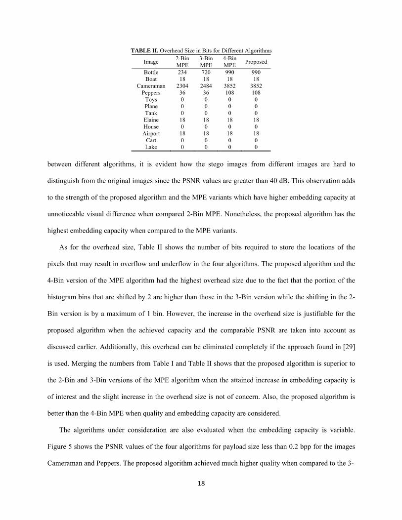
TABLE II. Overhead Size in Bits for Different Algorithms
Image 2-Bin MPE
3-Bin MPE
4-Bin MPE Proposed
Bottle 234 720 990 990 Boat 18 18 18 18
Cameraman 2304 2484 3852 3852 Peppers 36 36 108 108
Toys 0 0 0 0 Plane 0 0 0 0 Tank 0 0 0 0
Elaine 18 18 18 18 House 0 0 0 0 Airport 18 18 18 18
Cart 0 0 0 0 Lake 0 0 0 0
between different algorithms, it is evident how the stego images from different images are hard to
distinguish from the original images since the PSNR values are greater than 40 dB. This observation adds
to the strength of the proposed algorithm and the MPE variants which have higher embedding capacity at
unnoticeable visual difference when compared 2-Bin MPE. Nonetheless, the proposed algorithm has the
highest embedding capacity when compared to the MPE variants.
As for the overhead size, Table II shows the number of bits required to store the locations of the
pixels that may result in overflow and underflow in the four algorithms. The proposed algorithm and the
4-Bin version of the MPE algorithm had the highest overhead size due to the fact that the portion of the
histogram bins that are shifted by 2 are higher than those in the 3-Bin version while the shifting in the 2-
Bin version is by a maximum of 1 bin. However, the increase in the overhead size is justifiable for the
proposed algorithm when the achieved capacity and the comparable PSNR are taken into account as
discussed earlier. Additionally, this overhead can be eliminated completely if the approach found in [29]
is used. Merging the numbers from Table I and Table II shows that the proposed algorithm is superior to
the 2-Bin and 3-Bin versions of the MPE algorithm when the attained increase in embedding capacity is
of interest and the slight increase in the overhead size is not of concern. Also, the proposed algorithm is
better than the 4-Bin MPE when quality and embedding capacity are considered.
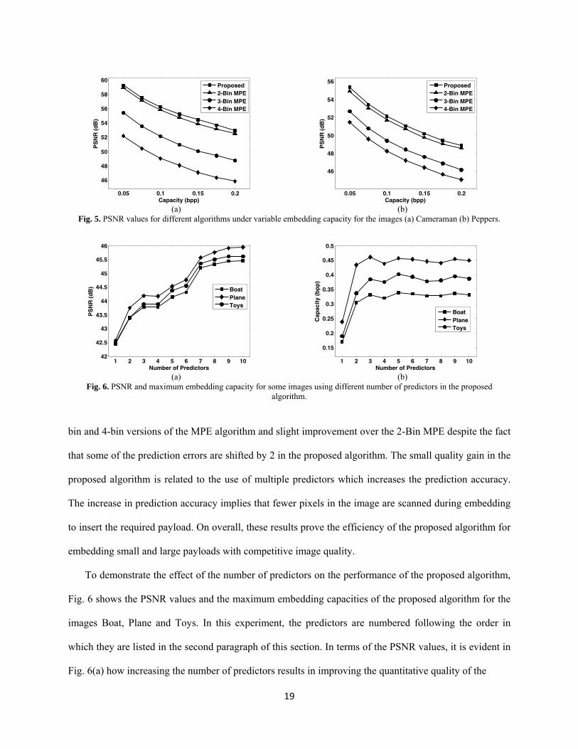
The algorithms under consideration are also evaluated when the embedding capacity is variable.
Figure 5 shows the PSNR values of the four algorithms for payload size less than 0.2 bpp for the images
Cameraman and Peppers. The proposed algorithm achieved much higher quality when compared to the 3-
19
0.05 0.1 0.15 0.2
46
48
50
52
54
56
58
60
Capacity (bpp)
PS
NR
(d
B)
Proposed2-Bin MPE3-Bin MPE4-Bin MPE
(a)
0.05 0.1 0.15 0.2
46
48
50
52
54
56
Capacity (bpp)
PS
NR
(d
B)
Proposed2-Bin MPE3-Bin MPE4-Bin MPE
(b)
Fig. 5. PSNR values for different algorithms under variable embedding capacity for the images (a) Cameraman (b) Peppers.
1 2 3 4 5 6 7 8 9 1042
42.5
43
43.5
44
44.5
45
45.5
46
Number of Predictors
PS
NR
(d
B)
BoatPlaneToys
(a)
1 2 3 4 5 6 7 8 9 10
0.15
0.2
0.25
0.3
0.35
0.4
0.45
0.5
Number of Predictors
Cap
acit
y (b
pp
)
BoatPlaneToys
(b)
Fig. 6. PSNR and maximum embedding capacity for some images using different number of predictors in the proposed algorithm.
bin and 4-bin versions of the MPE algorithm and slight improvement over the 2-Bin MPE despite the fact
that some of the prediction errors are shifted by 2 in the proposed algorithm. The small quality gain in the
proposed algorithm is related to the use of multiple predictors which increases the prediction accuracy.
The increase in prediction accuracy implies that fewer pixels in the image are scanned during embedding
to insert the required payload. On overall, these results prove the efficiency of the proposed algorithm for
embedding small and large payloads with competitive image quality.
To demonstrate the effect of the number of predictors on the performance of the proposed algorithm,
Fig. 6 shows the PSNR values and the maximum embedding capacities of the proposed algorithm for the
images Boat, Plane and Toys. In this experiment, the predictors are numbered following the order in
which they are listed in the second paragraph of this section. In terms of the PSNR values, it is evident in
Fig. 6(a) how increasing the number of predictors results in improving the quantitative quality of the

20
1 2 3 4 5 6 7 8 9 100
2
4
6
8
10
12
14
16x 10
4
Number of PredictorsC
ou
nt
Positive ErrorsNegative ErrorsBipolar Errors
Fig. 7. Distribution of prediction errors for the Boat image using different number of predictors.
stego image. This can be justified by considering the distribution of the prediction errors values shown in
Fig. 7 for the Boat image. Increasing the number of predictors reduces the occasions in which the
prediction errors from different predictors are unipolar. This implies that the cases in which the prediction
errors are shifted by 2 are less during the embedding procedure are reduced.
Regarding the maximum embedding capacity, the curves in Fig. 6(b) show how the capacity jumps
significantly when moving from a single predictor to more predictors. However, using more predictors
does not always add to the embedding capacity. For example, the best embedding capacity for the Boat
image is achieved when three predictors are used. Nonetheless, using more predictors significantly
improves the quality of the stego image for the reason discussed in the previous paragraph and as shown
by the PSNR curves in Fig. 6(a). It is worth to mention here that the numbers presented in Fig. 6 can be
improved by finding an optimal set of predictors over the entire image through exhaustive search in set of
given predictors. However this adds to the computational cost of the algorithm during the embedding
procedure.
Finally, Table III shows the average time required to process the 12 images shown before when
different number of predictors are used in the proposed algorithm. Regarding the 2-Bin, 3-Bin and 4-Bin
MPE algorithms, the average processing time was 8.40, 8.52 and 8.59 seconds, respectively. It is expected
that the processing time of the proposed algorithm is higher than the MPE-based algorithms even when
fewer predictors are employed. This is related to the way the embedding and extraction procedures are
designed since they involve the computation of the minimum, maximum, or the median of the prediction

21
Table III. Average Embedding Time Using Different Number of Predictors in the Proposed Algorithm No. Predictors Time (Seconds)
1 9.76 2 12.20 3 13.45 4 15.50 5 18.56 6 20.26 7 22.24 8 24.55 9 29.13 10 31.79
errors at each pixel that is considered for embedding. However, the achieved increase in the embedding
capacity and the satisfactory image quality for the proposed algorithm makes it suitable for data hiding in
time-insensitive or offline applications.
4. Conclusion
In this paper, an efficient reversible data hiding scheme is proposed. The algorithm is essentially based on
histogram shifting of prediction errors. In contrast to similar algorithms that exist in the literature, the
proposed algorithm employs the use of multiple predictors instead of a single one. The rationale behind
that is improving the prediction accuracy which in turn affects the embedding capacity and the quality of
the stego image. Integrating multiple predictors is performed in way to guarantee the reversibility and at
no additional cost in terms of the overhead information that is required in order to extract the watermark
and recover the original image. The proposed algorithm is shown to provide significant increase in the
embedding capacity with satisfactory quantitative and visual quality.
References
[1] C. I. Podilchuk and E. J. Delp, “Digital watermarking: Algorithms and applications,” IEEE Signal Process.
Mag., vol. 18, no. 4, pp. 33-46, Jul. 2001.
[2] S. H. Liu, T. H. Chen, H. X. Yao and W. Gao, “A variable depth LSB data hiding technique in images,” Proc.
International Conference on Machine Learning and Cybernetics, Aug. 2004, pp. 3990-3994.
[3] H. C. Wu, N. I. Wu, C. S. Tsai, M. S. Hwang, “Image steganographic scheme based on pixel-value
differencing and LSB replacement methods,” Proc. IEE Vision, Image, and Signal Processing, Oct. 2005, vol.
152, issue 5, pp.611 – 615.
22
[4] Y. H. Yu, C. C. Chang, and Y. C. Hu, “Hiding secret data in images via predictive coding,” Pattern
Recognition, vol. 38, no. 5, pp. 691–705, May 2005.
[5] B. Yang, M. Schmucker, W. Funk, C. Busch, & S. Sun, “Integer DCT-Based reversible watermarking for
images using companding technique,” Proc. SPIE 5306, Security, Steganography, and Watermarking of
Multimedia Contents VI , Jan. 2004, USA, pp. 405-415.
[6] J. M. Barton, “Method and apparatus for embedding authentication information within digital data,” U.S.
Patent 5,646,997, Jul. 1997.
[7] J. Fridrich, M. Goljan and R. Du, “Invertible authentication,” Proc. SPIE, Security and Watermarking of
Multimedia Contents, Jan. 2001, USA, pp. 197-208.
[8] J. Tian, "Reversible data embedding using a difference expansion," IEEE Trans. on Circuits and Systems for
Video Technology, vol.13, no.8, pp. 890- 896, Aug. 2003.
[9] A. M. Alattar, "Reversible watermark using difference expansion of quads," Proc. Acoustics, Speech, and
Signal Processing (ICASSP '04), May 2004, vol.3, pp. 377-380.
[10] A. M. Alattar, "Reversible watermark using the difference expansion of a generalized integer transform," IEEE
Trans. on Image Processing, , vol.13, no.8, pp.1147-1156, Aug. 2004.
[11] Z. Ni, Y. Q. Shi, N. Ansari and W. Su, “Reversible data hiding,” IEEE Trans. on Circuits and Systems for
Video Technology, vol.16, no.3, pp.354-362, Mar. 2006.
[12] M. Fallahpour and M. H. Sedaaghi, “High capacity lossless data hiding based on histogram modification,”
IEICE Electronics Express, vol. 4, no. 7, pp. 205-210, Apr. 2007.
[13] C. C. Lin and N. L. Hsueh, “Hiding data reversibly in an image via increasing differences between two
neighboring pixels,” IEICE Trans. on Information and Systems, vol. E90-D, no. 12, pp. 2053-2059, Dec. 2007.
[14] W. Hong, T. -S. Chen, C. -W. Shiu, “Reversible data hiding for high quality images using modification of
prediction errors,” The Journal of Systems and Software, vol. 82, no. 11, pp. 1833-1842, Nov. 2009.
[15] S. –K. Yip, O. C. Au, C. –W. Ho and H. –M. Wong,“ Content adaptive watermarking using a 2-stage
predictor,” Proc. IEEE International Conference on Image Processing (ICIP), Italy, Sept. 2005, vol. 3, pp. 953-
956.
[16] S. -S. Wang, S. –J. Fan and C. –S. Li, “A New reversible data hiding based on fuzzy predictor,” Proc. of 2012
International Conference on Fuzzy Theory and Its Applications, Taiwan, Nov. 2012, pp. 258-262.

23
[17] C. –L. Liu and T. –H. Lai, “A Novel reversible data hiding method using least-square based predictor,” 2012
International Symposium on Computer, Consumer and Control (IS3C), Taiwan, Jun. 2012, pp. 448-451.
[18] S. –K. Yip, O. C. Au, H. –M. Wong and C. –W. Ho, “Generalized Lossless Data Hiding By Multiple
Predictors,” Proc. IEEE International Symposium on Circuits and Systems, Greece, May. 2006, pp. 1426-1429.
[19] C. –F. Lee, H.-L. Chen and H. –K. Tso, “Embedding capacity raising in reversible data hiding based on
prediction of difference expansion,” Journal of Systems and Software, vol. 83, no. 10, pp. 1864–1872, Oct.
2010.
[20] Y. Luo, F. Peng, X. Li and B. Yang, “Reversible image watermarking based on prediction error-expansion and
compensation,” Proc. IEEE International Conference on Multimedia and Expo (ICME), Spain, Jul. 2011, pp. 1
– 6.
[21] C.-H. Yang, F.-H. Hsu, M.-H. Wu and S.-J. Wang, “Improving histogram-based reversible data hiding by
tictactoemidlet predictions,” Proc. Fourth International Conference on Genetic and Evolutionary Computing,
China, Dec. 2010, pp. 667 – 670.
[22] G. Xuan, Y.Q. Shi, J. Teng, X. Tong and P. Chai, “Double-threshold reversible data hiding,” Proc. IEEE
International Symposium on Circuits and Systems, France, May 2010, pp. 1129 – 1132.
[23] L. Luo, Z. Chen, M. Chen, X. Zeng, and Z. Xiong, “Reversible image watermarking using interpolation
technique,” IEEE Trans. on Information Forensics and Security, vol. 5, no. 1, pp. 187–193, 2010.
[24] Y. –C. Chou and H. –C. Li, “High payload reversible data hiding scheme using difference segmentation and
histogram shifting,” Journal of Electronic Science and Technology, vol. 11, no. 1, Mar. 2008.
[25] M. Wienberger, G. Seroussi, and G. Sapiro, “LOCO-I: A Low complexity, context Based, lossless image
compression algorithm,” Proc. of Data Compression, USA, Apr.1996, pp. 140-149.
[26] J. Jiang, B. Guo and S. Yang, “Revisiting the JPEG-LS prediction scheme,” Proc. IEE Vision, Image and
Signal Processing, vol. 147, no. 6, pp. 575- 580, Dec. 2000.
[27] R.C. Gonzalez, R.E. Woods, Digital Image Processing. Upper Saddle River, NJ, Prentice Hall, 2002.
[28] Calibrated Imaging Lab, http://www.cs.cmu.edu/~cil/v-images.html, Last accessed December 2013.
[29] I. Jafar, S. Hiary and K. Darabkh, “An Improved Reversible Data Hiding Algorithm Based on Modification of
Prediction Errors,” Proceedings of the 6th International Conference on Digital Image Processing (ICDIP),
Greece, April 2014.


