
Laboratorio Subterráneo de Canfranc (Huesca), 27-28-29 March 2014
Electromagnetic analysis of microwave cavities for dark-matter axion detectors
Benito Gimeno(1), Daniel González-Iglesias (1), Juan Pastor Graells(1), Ángel San Blas Oltra(2), José Manuel Catalá(3),Vicente E. Boria(3)
, Jordi Gil(4), Carlos P. Vicente(4)
(1) University of Valencia, Spain (2) University Miguel Hernández of Elche (Alicante), Spain (3) Technical University of Valencia, Spain (4) AURORASAT, S.L., Valencia, Spain
1

Laboratorio Subterráneo de Canfranc (Huesca), 27-28-29, March 2014
INDEX
2
• Introduction
• The rectangular waveguide
• The empty rectangular cavity
• Excitation of microwave cavities: coupling
• The BI-RME method
• Examples
• Conclusions

Laboratorio Subterráneo de Canfranc (Huesca), 27-28-29, March 2014
INDEX
3
• Introduction
• The rectangular waveguide
• The empty rectangular cavity
• Excitation of microwave cavities: coupling
• The BI-RME method
• Examples
• Conclusions

Laboratorio Subterráneo de Canfranc (Huesca), 27-28-29, March 2014 4
Introduction
• During these days we have been talking about dark matter axions, now the question is: how to detect them? • Microwave resonators have been proposed in the literature for dark-matter axions detectors. • The objective of this talk is to review the most relevant feautures and performances of microwave cavities
from the theoretical perspective of the Classical Electrodynamics, in order to analyze their applications in the research field of axion detectors physics.

Laboratorio Subterráneo de Canfranc (Huesca), 27-28-29, March 2014
INDEX
5
• Introduction
• The rectangular waveguide
• The empty rectangular cavity
• Excitation of microwave cavities: coupling
• The BI-RME method
• Examples
• Conclusions

Laboratorio Subterráneo de Canfranc (Huesca), 27-28-29, March 2014 6
The rectangular waveguide
• The complete set of solenoidal modes of an empty rectangular cavity can be obtained short-circuiting both sides of a rectangular waveguide.
• The modes of a rectangular waveguide are wellknown:
x a
b
y
z
( )
( )
0
expcossin
expsincos
2,
0
2,
0
=
−
−=−=
−
==
z
zmnc
mnxTEy
zmnc
mnyTEx
E
zyb
nx
a
m
a
m
k
jBHZE
zyb
nx
a
m
b
n
k
jBHZE
γπππωµ
γπππωµ
( )
( )
( )zyb
nx
a
mBH
zyb
nx
a
m
b
n
kBH
zyb
nx
a
m
a
m
kBH
zmnz
zmnc
zmny
zmnc
zmnx
γππ
γπππγ
γπππγ
−
=
−
=
−
=
expcoscos
expsincos
expcossin
2,
2,
TEz modes:

Laboratorio Subterráneo de Canfranc (Huesca), 27-28-29, March 2014 7
The rectangular waveguide
TMz modes:
( )
( )
( )zyb
nx
a
mAE
zyb
nx
a
m
b
n
kAE
zyb
nx
a
m
a
m
kAE
zmnz
zmnc
zmny
zmnc
zmnx
γππ
γπππγ
γπππγ
−
=
−
−=
−
−=
expsinsin
expcossin
expsincos
2,
2,
( ) ( )
( ) ( )
0
expsincos1
expcossin1
2,
00
2,
0
=
−
−
−==
−
−
=−=
z
zmnc
rmn
TM
xy
zmnc
rmn
TM
yx
H
zyb
nx
a
m
a
m
k
jtgjA
Z
EH
zyb
nx
a
m
b
n
k
jtgjA
Z
EH
γπππδεεωε
γπππδεωε
Relevant relationships of the rectangular waveguide (uniformly dielectric loaded):
22,
2zmnckk γ−=
22
,
+
=
b
n
a
mk mnc
ππ
zzmncz jkk βαγ +=−= 22,
( )δεεµω jtgk r −= 10022
εεδ
′′′
=tg
( ) ηγδεωε
γjkjtgj
Z z
r
zTM =
−=
10
ηγγ
ωµ
zzTE
jkjZ == 0
( )δεεµη
jtgr −=
10
0

Laboratorio Subterráneo de Canfranc (Huesca), 27-28-29, March 2014 8
The rectangular waveguide
Modal spectrum of a rectangular waveguide for different ratio b/a:

Laboratorio Subterráneo de Canfranc (Huesca), 27-28-29, March 2014 9
The rectangular waveguide
The fundamental TEz10 mode:
( )( ) z
ctTEt
zzt
ct
zz
eyxa
senf
fBjzHZE
exxa
sena
BHk
H
exa
BH
⋅
⋅
⋅
⋅⋅
⋅⋅⋅
⋅⋅−=±⋅=
⋅⋅
⋅⋅
⋅⋅±=⋅∇⋅=
⋅
⋅⋅=
γ
γ
γ
πη
ππ
γγ
π
ˆˆx
ˆ
cos
2
ac 2=λ 2
1εµ ⋅⋅⋅
=a
fc
22
22 εµωπγ ⋅⋅−
=−=
akkc
riorioc
i εεµµωλπγ 2
22
−
⋅=
12
−
=
ff
Z
c
TE
η

Laboratorio Subterráneo de Canfranc (Huesca), 27-28-29, March 2014 10
The rectangular waveguide
Electromagnetic fields distribution of a rectangular waveguide with b=a/2:
Laboratorio Subterráneo de Canfranc (Huesca), 27-28-29, March 2014 11
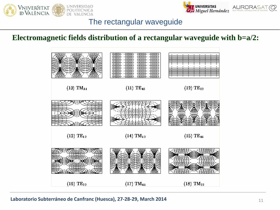
The rectangular waveguide
Electromagnetic fields distribution of a rectangular waveguide with b=a/2:

Laboratorio Subterráneo de Canfranc (Huesca), 27-28-29, March 2014
INDEX
12
• Introduction
• The rectangular waveguide
• The empty rectangular cavity
• Excitation of microwave cavities: coupling
• The BI-RME method
• Examples
• Conclusions

Laboratorio Subterráneo de Canfranc (Huesca), 27-28-29, March 2014 13
The empty rectangular cavity
• The complete set of solenoidal modes of an empty rectangular cavity can
be obtained short-circuiting both sides of a rectangular waveguide:
Short-circuit 1
L
Short-circuit 2

Laboratorio Subterráneo de Canfranc (Huesca), 27-28-29, March 2014 14
The empty rectangular cavity
• The cavity modes can be easily constructed as the superposition of an
incident wave and a reflected wave:
( )( )zjzjt eeyxEE ββ ρ−= −,0
( )( ) ( )( )zjzjz
zjzjt eeyxHeeyxHH ββββ ρρ −++= −− ,, 00
TEz modes:
with ρ=1
0
sincossin
sinsincos
2,
0
2,
0
=
−=
=
z
mncmny
mncmnx
E
zL
py
b
nx
a
m
a
m
kBE
zL
py
b
nx
a
m
b
n
kBE
ππππωµ
ππππωµ
−=
=
=
zL
py
b
nx
a
mjBH
zL
py
b
nx
a
m
b
n
k
jBH
zL
py
b
nx
a
m
a
m
k
jBH
mnz
mnc
zmny
mnc
zmnx
πππ
ππππβ
ππππβ
sincoscos
cossincos
coscossin
2,
2,
m=0,1,2… ; n=0,1,2…; p=1,2,3… (the case m=n=0 is not allowed)
Laboratorio Subterráneo de Canfranc (Huesca), 27-28-29, March 2014 15
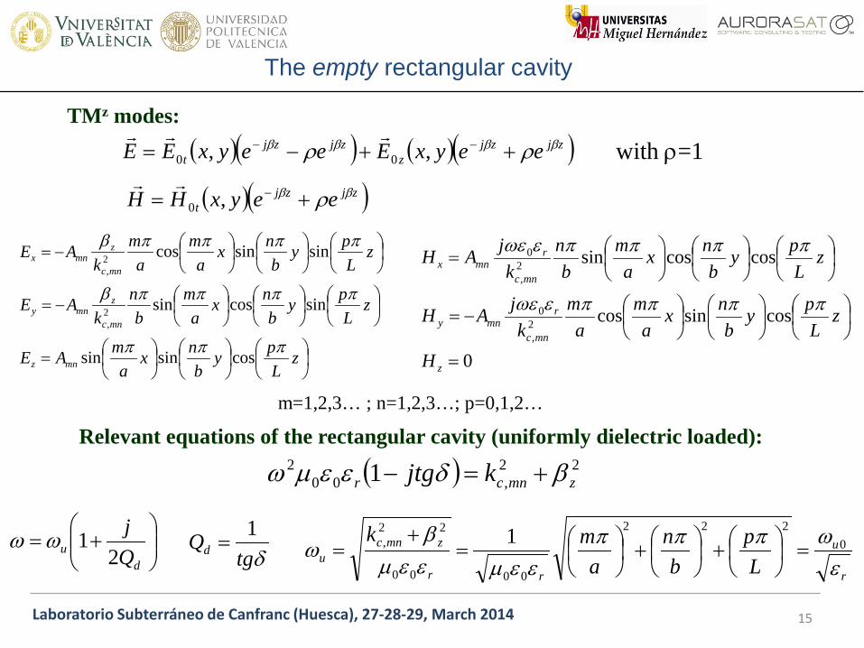
The empty rectangular cavity
( )( ) ( )( )zjzjz
zjzjt eeyxEeeyxEE ββββ ρρ ++−= −− ,, 00
( )( )zjzjt eeyxHH ββ ρ+= −,0
TMz modes:
=
−=
−=
zL
py
b
nx
a
mAE
zL
py
b
nx
a
m
b
n
kAE
zL
py
b
nx
a
m
a
m
kAE
mnz
mnc
zmny
mnc
zmnx
πππ
ππππβ
ππππβ
cossinsin
sincossin
sinsincos
2,
2,
0
cossincos
coscossin
2,
0
2,
0
=
−=
=
z
mnc
rmny
mnc
rmnx
H
zL
py
b
nx
a
m
a
m
k
jAH
zL
py
b
nx
a
m
b
n
k
jAH
ππππεωε
ππππεωε
with ρ=1
m=1,2,3… ; n=1,2,3…; p=0,1,2…
Relevant equations of the rectangular cavity (uniformly dielectric loaded):
( ) 22,00
2 1 zmncr kjtg βδεεµω +=−
+=
du Q
j
21ωω
δtgQd
1=
r
u
rr
zmncu L
p
b
n
a
mk
εωπππ
εεµεεµβ
ω 0
222
0000
22, 1
=
+
+
=
+=
Laboratorio Subterráneo de Canfranc (Huesca), 27-28-29, March 2014 16
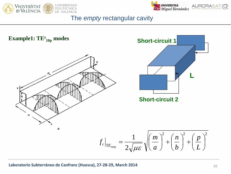
The empty rectangular cavity
222
2
1
+
+
=
L
p
b
n
a
mf
mnpTEr µε
Short-circuit 1
L
Short-circuit 2
Example1: TEz10p modes

Laboratorio Subterráneo de Canfranc (Huesca), 27-28-29, March 2014 17
The empty rectangular cavity
Example2: Rectangular cavity in WR-340 a=86.36 mm, b=43.18 mm
p L (mm.)1 86.72 173.43 260.14 346.85 433.56 520.17 606.88 693.59 780.210 866.911 953.6
GHzL
p
af
pTEr 45.21
2
122
10=
+
=
µε

Laboratorio Subterráneo de Canfranc (Huesca), 27-28-29, March 2014 18
The empty rectangular cavity
• The time-average electric and magnetic energies stored by each mode of a
microwave cavity are given by:
which can be calculated for both family of rectangular modes:
∫ ∫cc V
rV
re dVEdVEEW
200
44
εεεε=⋅= ∗ ∫ ∫
cc VVm dVHdVHHW2
00
44
µµ=⋅= ∗
nmmnc
umnre
abL
k
BW εεµωεε
84 2,
20
220=
+=
2,
220 1
84 mnc
znmmnm k
abLBW
βεεµ
≠=
=0,1
0,2
p
ppε
+=
2,
220 1
84 mnc
zpmn
re k
abLAW
βεεεp
mnc
rumnm
abL
k
AW εεεωµ
84 2,
220
220=
≠=
=0,1
0,2
p
ppε
TMz modes:
TEz modes:

Laboratorio Subterráneo de Canfranc (Huesca), 27-28-29, March 2014 19
The empty rectangular cavity
• The power dissipated within a microwave cavity considering losses in the
metallic walls as well as in a uniform lossy dielectric filling the cavity are
given by:
δεωεεωεσ tgre 00 =′′= ∫cV
ed dSEP
2
2
σ= ∫
cSs dSH
RP
2
tan0 2
=
• The quality factor of a microwave cavity is defined as follows:
ud
med P
WWQ
ωω
ω=
+=
δσεεω
tgQ
e
rud
10 ==
uPP
WWQ
d
meu
ωω
ω=
++
=0 dcu QQQ
111+=

Laboratorio Subterráneo de Canfranc (Huesca), 27-28-29, March 2014
INDEX
20
• Introduction
• The rectangular waveguide
• The empty rectangular cavity
• Excitation of microwave cavities: coupling
• The BI-RME method
• Examples
• Conclusions

Laboratorio Subterráneo de Canfranc (Huesca), 27-28-29, March 2014
Excitation of microwave cavities: coupling
21
• An empty microwave cavity has to be feeded with an external component in
order to excite an electromagnetic field within the cavity. • There are different mechanisms to excite a microwave cavity: - Waveguide Iris (holes performed on one cavity wall):
Magnetic (a) and electric (b) coupling apertures

Laboratorio Subterráneo de Canfranc (Huesca), 27-28-29, March 2014 22
Excitation of microwave cavities: coupling
Example1: Inductive band-pass filter implemented in rectangular waveguide for LMDS technology at 28 GHz
Courtesy of ESTEC-ESA

Laboratorio Subterráneo de Canfranc (Huesca), 27-28-29, March 2014 23
Excitation of microwave cavities: coupling
Example2: Dual-mode band-pass filter implemented in circular waveguide with elliptical irises for space telecommunications applications
Frequency Adjustment
Dual-mode Coupling
Input/Output Couplings
Inter-Cavity Couplings
B. Gimeno, M. Guglielmi, “Full Wave Network Representation for Rectangular, Circular, and Elliptical to Elliptical Waveguide Junctions”, IEEE Transactions on Microwave Theory and Techniques , vol. 45, no. 3, pp. 376-384, March 1997

Laboratorio Subterráneo de Canfranc (Huesca), 27-28-29, March 2014 24
Excitation of microwave cavities: coupling
Manufactured prototype (courtesy by ESA-ESTEC): ESA PATENT: “Alternative implementation for dual-mode filters in circular
waveguide”, reference number: 9606337, EU-USA-Canada

Laboratorio Subterráneo de Canfranc (Huesca), 27-28-29, March 2014 25
Excitation of microwave cavities: coupling
Electrical response: comparison between theory (left) and experiment (right)

Laboratorio Subterráneo de Canfranc (Huesca), 27-28-29, March 2014 26
Excitation of microwave cavities: coupling
Example3: Coupled-Cavities band-pas filter with tuneable response for space telecommunications applications
Manufactured Prototype
Courtesy of ESTEC-ESA

Laboratorio Subterráneo de Canfranc (Huesca), 27-28-29, March 2014 27
Excitation of microwave cavities: coupling
Comparison between theory (up) and experiment (down)

Laboratorio Subterráneo de Canfranc (Huesca), 27-28-29, March 2014 28
Excitation of microwave cavities: coupling
Example4: Cuasi-inductive band-pass filter with rounded corners for space telecommunications applications
Cut Planes
Pieces to be manufactured
Design Parameters: li , ti (High Efficiency) Low Losses: Location of Cut Planes

Laboratorio Subterráneo de Canfranc (Huesca), 27-28-29, March 2014 29
Excitation of microwave cavities: coupling
Detailed View of a Piece
Assembling Process
of the Pieces
Prototype Pieces
Courtesy of ESTEC-ESA

Laboratorio Subterráneo de Canfranc (Huesca), 27-28-29, March 2014 30
Excitation of microwave cavities: coupling
Comparison between theory and experiment

Laboratorio Subterráneo de Canfranc (Huesca), 27-28-29, March 2014 31
Excitation of microwave cavities: coupling
- Electric probe: Coaxial probe inserted in the cavity

Laboratorio Subterráneo de Canfranc (Huesca), 27-28-29, March 2014 32
Excitation of microwave cavities: coupling
Example1: Connector between a coaxial transmission line and a rectangular waveguide

Laboratorio Subterráneo de Canfranc (Huesca), 27-28-29, March 2014 33
Excitation of microwave cavities: coupling
Example2: Inductive band-pass filter excited with a coaxial connector

Laboratorio Subterráneo de Canfranc (Huesca), 27-28-29, March 2014 34
Excitation of microwave cavities: coupling
Example3: Analysis of comb-line diplexers excited with coaxial connectors for space telecommunication subsystems

Laboratorio Subterráneo de Canfranc (Huesca), 27-28-29, March 2014 35
Excitation of microwave cavities: coupling

Laboratorio Subterráneo de Canfranc (Huesca), 27-28-29, March 2014 36
Excitation of microwave cavities: coupling
- Magnetic current loop: current loop contacting the metallic surface of the cavity

Laboratorio Subterráneo de Canfranc (Huesca), 27-28-29, March 2014 37
Excitation of microwave cavities: coupling
Examples: There are a lot of different kind of current loops used in microwave circuits

Laboratorio Subterráneo de Canfranc (Huesca), 27-28-29, March 2014
INDEX
38
• Introduction
• The rectangular waveguide
• The empty rectangular cavity
• Excitation of microwave cavities: coupling
• The BI-RME method
• Examples
• Conclusions

Laboratorio Subterráneo de Canfranc (Huesca), 27-28-29, March 2014
The BI-RME method
39
• BI-RME: Boundary-Integral Resonant Mode Expansion • Method developed at University of Pavia (Italy) by Prof. Giuseppe
Conciauro, Prof. Marco Bressan, and Prof. Paolo Arcioni: G. Conciauro, M. Guglielmi, R. Sorrentino, Advanced Modal Analysis, Wiley, 2000 • During last 20 years it has been applied to the rigorous and efficient modal
analysis of uniform arbitrarily-shaped waveguides (BI-RME 2D), and cavities including metallic and dielectric objects with arbitrary shape (BI-RME 3D).
• There are more than 50 articles published in international journals and
transactions directly related with BI-RME applications.

Laboratorio Subterráneo de Canfranc (Huesca), 27-28-29, March 2014
The BI-RME method
40
• Both versions of the BI-RME method transform an integral equation of Fredholm of first kind into an algebraic eigenvalue problem which is numerically solved with standard diagonalization subrutines.
• Example of BI-RME 2D: computation of the full modal spectrum of a ridge rectangular waveguide. The cutoff frequencies (eigenvalues) and the electromagnetic fields (eigenvectors) are computed for a set of modes.
S. Cogollos, S. Marini, V. E. Boria, P. Soto, A. Vidal, H. Esteban, J. V. Morro, B. Gimeno, ‘Efficient Modal Analysis of Arbitrarily Shaped Waveguides Composed of Linear, Circular, and Elliptical Arcs Using the BI-RME Method’, IEEE Transactions on Microwave Theory and Techniques, vol. 51, no. 12, pp. 2378-2390, Dec. 2003
TE10 TM11

Laboratorio Subterráneo de Canfranc (Huesca), 27-28-29, March 2014
The BI-RME method
41
• Example1 of BI-RME 3D: computation of the full modal spectrum of a rectangular microwave cavity loaded with a metallic cylindrical ‘mushroom’. The resonant frequencies (eigenvalues) and the electromagnetic fields (eigenvectors) are computed for a set of modes.
F. Mira, M. Bressan, G. Conciauro, B. Gimeno, V. E. Boria, ‘Fast S-Domain Modeling of Rectangular Waveguides With Radially Symmetric Metal Insets’, IEEE Transactions on Microwave Theory and Techniques, vol. 53, no. 4, pp. 1294-1303, April 2005
a=30.00mm b=15.00mm c=20.00mm dt=4.00mm di=8.00mm de=12.00mm hi=7.00mm he=10.00mm ht=10.00mm

Laboratorio Subterráneo de Canfranc (Huesca), 27-28-29, March 2014
The BI-RME method
42
First mode Second mode
Third mode Fourth mode
Electric field lines and surface current density lines have been plotted.
Laboratorio Subterráneo de Canfranc (Huesca), 27-28-29, March 2014
The BI-RME method
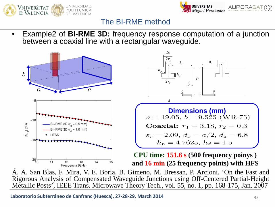
43
• Example2 of BI-RME 3D: frequency response computation of a junction between a coaxial line with a rectangular waveguide.
Á. A. San Blas, F. Mira, V. E. Boria, B. Gimeno, M. Bressan, P. Arcioni, ‘On the Fast and Rigorous Analysis of Compensated Waveguide Junctions using Off-Centered Partial-Height Metallic Posts’, IEEE Trans. Microwave Theory Tech., vol. 55, no. 1, pp. 168-175, Jan. 2007
CPU time: 151.6 s (500 frequency poinys ) and 16 min (25 frequency points) with HFS
Dimensions (mm)

Laboratorio Subterráneo de Canfranc (Huesca), 27-28-29, March 2014
The BI-RME method
44
• Example3 of BI-RME 3D: calculation of the resonant modes of the
ELETTRA accelerating cavity placed in Stanford Linear Accelerator
(USA).
P. Arcioni, M. Bressan, L.Perregrini, ‘A New Boundary Integral Approach to the Determination of the Resonant Modes of Arbitraily Shaped Cavities’, IEEE Trans. Microwave Theory Tech., vol. 43, no. 8, pp. 1848-1855, Aug. 1995
Laboratorio Subterráneo de Canfranc (Huesca), 27-28-29, March 2014
The BI-RME method
45
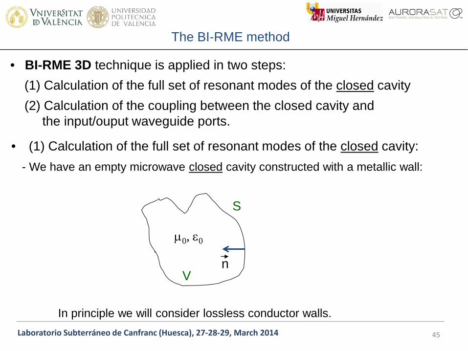
• BI-RME 3D technique is applied in two steps:
(1) Calculation of the full set of resonant modes of the closed cavity
(2) Calculation of the coupling between the closed cavity and the input/ouput waveguide ports.
• (1) Calculation of the full set of resonant modes of the closed cavity:
- We have an empty microwave closed cavity constructed with a metallic wall:
In principle we will consider lossless conductor walls.
V
S
n
µ0, ε0

Laboratorio Subterráneo de Canfranc (Huesca), 27-28-29, March 2014
The BI-RME method
46
- Maxwell equations (expressed in frequency domain) gobern the electromagnetic
fields existing within the cavity, ρ and J being the time-harmonic electric sources
(representing a metallic inset inside the cavity):
- The total electromagnetic field inside the cavity can be expressed as a
superposition of solenoidal and irrotational modes:
where En, Fn, Hn and Gn are the expansion coefficients.

Laboratorio Subterráneo de Canfranc (Huesca), 27-28-29, March 2014
The BI-RME method
47
- The normalized modal vectors are clasified in 4 groups:
Solenoidal electric modes (resonant modes):
Irrotational electric modes (non-resonant modes):
Boundary condition on the cavity surface:
Boundary condition on the cavity surface:
, on the cavity surface
PHYSICAL RESONANCES

Laboratorio Subterráneo de Canfranc (Huesca), 27-28-29, March 2014
The BI-RME method
48
Solenoidal magnetic modes (resonant modes):
Irrotational magnetic modes (non-resonant modes):
Boundary condition on the cavity surface:
Boundary condition on the cavity surface:
- Solenoidal electric and magnetic modes satisfy these reciprocal equations:
, on the cavity surface
Laboratorio Subterráneo de Canfranc (Huesca), 27-28-29, March 2014
The BI-RME method
49
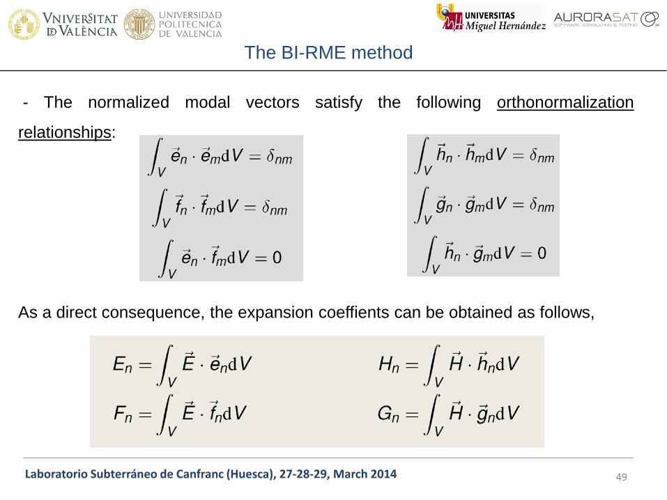
- The normalized modal vectors satisfy the following orthonormalization
relationships:
As a direct consequence, the expansion coeffients can be obtained as follows,

Laboratorio Subterráneo de Canfranc (Huesca), 27-28-29, March 2014
The BI-RME method
50
- Next step is to expand the curl of the electric (magnetic) field as a magnetic-like
(electric-like) field function. After inserting these results in Maxwell equations we find:
which allows to obtain the expansion coefficients and Gm = 0.

Laboratorio Subterráneo de Canfranc (Huesca), 27-28-29, March 2014
The BI-RME method
51
- By combining the previous equations we find:
Therefore, the expressions of both electric scalar potential and magnetic vector
potential are written as
and
ELECTRIC SCALAR GREEN’S FUNCTION
IN THE COULOMB GAUGE

Laboratorio Subterráneo de Canfranc (Huesca), 27-28-29, March 2014
The BI-RME method
52
MAGNETIC DIADIC GREEN’S FUNCTION
IN THE COULOMB GAUGE
A dyadic expression is a second-order contravariant cartesian tensor defined in R3
which can be formulated in terms of a matrix:

Laboratorio Subterráneo de Canfranc (Huesca), 27-28-29, March 2014
The BI-RME method
53
- It can be easily demonstrated that the electric scalar potential in the Coulomb gauge
satisfies the Poisson differential equation:
As a consequence, the electric scalar Green’s function satisfies the following
differential equation:
whose solution can be splitted in a singular term and a regular one:
Laboratorio Subterráneo de Canfranc (Huesca), 27-28-29, March 2014
The BI-RME method
54
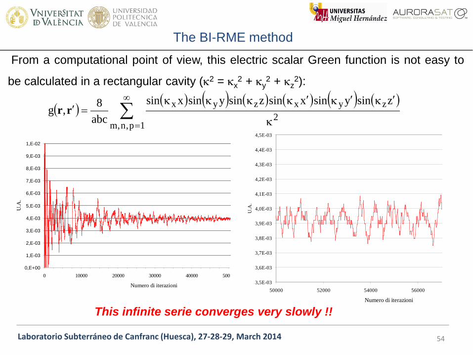
From a computational point of view, this electric scalar Green function is not easy to
be calculated in a rectangular cavity (κ2 = κx2 + κy
2 + κz2):
This infinite serie converges very slowly !!
( )( ) ( ) ( ) ( ) ( ) ( )
∑∞
= κ
′κ′κ′κκκκ=′
1p,n,m2
zyxzyx zsinysinxsinzsinysinxsin
abc
8,g rr
0,E+00
1,E-03
2,E-03
3,E-03
4,E-03
5,E-03
6,E-03
7,E-03
8,E-03
9,E-03
1,E-02
0 10000 20000 30000 40000 5000
Numero di iterazioni
U.A
.
3,5E-03
3,6E-03
3,7E-03
3,8E-03
3,9E-03
4,0E-03
4,1E-03
4,2E-03
4,3E-03
4,4E-03
4,5E-03
50000 52000 54000 56000
Numero di iterazioni
U.A
.

Laboratorio Subterráneo de Canfranc (Huesca), 27-28-29, March 2014
The BI-RME method
55
Ewald technique has to be used for an efficient computation of the infinite series:
P.P. Ewald, Ann der Physik, vol. 64, 1921
3D Gaussians distributions are added and substracted in order to improve convergence series
+
+
+
+
+
+
+
+
+
+
+
+
+
+
+
x
y
a
b
Images technique is used as an alternative
representation of the series
= +
ϕ 1 ϕ 2

Laboratorio Subterráneo de Canfranc (Huesca), 27-28-29, March 2014
The BI-RME method
56
Both series have to be treated in a very different way:
Solution in spectral domain
Solution in spatial domain
The argument of the serie exponentially vanishs when κ is increased
The argument of the series vanishs controled by the
erfc function (which tends to zero when R tends to • )

Laboratorio Subterráneo de Canfranc (Huesca), 27-28-29, March 2014
The BI-RME method
57
Exponential convergence for both series:
40 terms for ϕ 1 and 80 terms for ϕ 2
Efficient computacional efficiency: CPU time of 0.06 seconds for the same
accuracy than in the previous case

Laboratorio Subterráneo de Canfranc (Huesca), 27-28-29, March 2014
The BI-RME method
58
- It can also be easily demonstrated that the magnetic vector potential in the Coulomb gauge satisfies this differential equation:
As a consequence, the magnetic diadic Green’s function satisfies the following differential equation:
whose solution can be splitted in a singular term and a regular one (this is not trivial !!):

Laboratorio Subterráneo de Canfranc (Huesca), 27-28-29, March 2014
The BI-RME method
59
- Finally, electric and magnetic fields inside the cavity can be expressed in terms of integrals containing the aforementioned Green’s functions: where η=(µ0/ε0)1/2 is the free space characteristic impedance. Inserting expansions of both Green’s functions we find,

Laboratorio Subterráneo de Canfranc (Huesca), 27-28-29, March 2014
The BI-RME method
60
- Calculation of the resonant modes of the cavity is performed by imposing that the tangential component of the electric field is zero on the surface of the metallic obstacles contained in the cavity: This homogeneous system admits non-trivial solutions only for particular values of k, which are the resonant wavenumbers of the cavity. The surface current density J is the unknown function of this integral equation of Fredholm of first kind, and it has to be expanded as:
where wn and vn are a complete set of solenoidal and non-solenoidal vectorial basis functions defined on the surface of the metallic object, respectivelly.
Laboratorio Subterráneo de Canfranc (Huesca), 27-28-29, March 2014
The BI-RME method
61
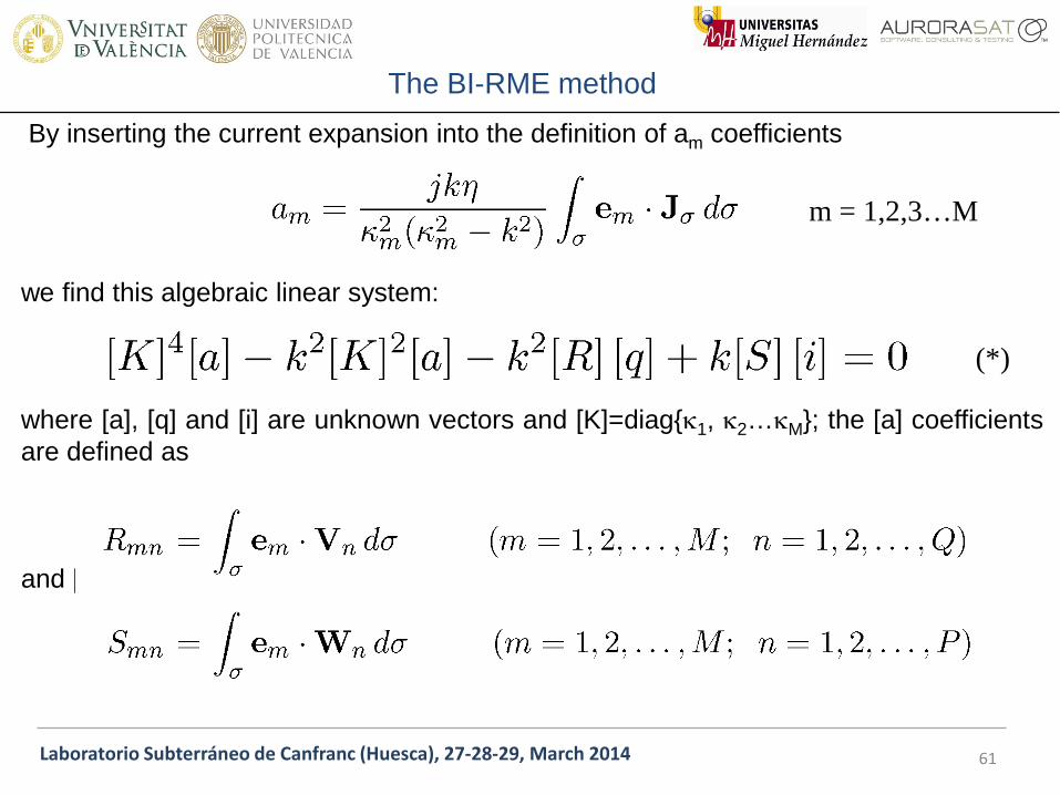
By inserting the current expansion into the definition of am coefficients we find this algebraic linear system: where [a], [q] and [i] are unknown vectors and [K]=diagκ1, κ2…κM; the [a] coefficients are defined as and [R] ,[S] are square matrices defined as:
m = 1,2,3…M
(*)

Laboratorio Subterráneo de Canfranc (Huesca), 27-28-29, March 2014
The BI-RME method
62
Using the Method of Moments with Galerkin technique (the expansion basis functions are used to dot-multiplying both sides of the integral equation) we find: where
(**)

Laboratorio Subterráneo de Canfranc (Huesca), 27-28-29, March 2014
The BI-RME method
63
The last equation allows to obtain Inserting this vector into (*) and (**) we find where

Laboratorio Subterráneo de Canfranc (Huesca), 27-28-29, March 2014
The BI-RME method
64
It can be demostrated that both matrices [A] and [B] are symmetric and definite positive, so the solution of the previous matricial equation has positive real eigenvalues, representing the solution of the problem. Electric and magnetic fields within the cavity can be calculated as:

Laboratorio Subterráneo de Canfranc (Huesca), 27-28-29, March 2014
The BI-RME method
65
- Calculation of the Q-factor of each resonant mode can be easily computed in this scenario:
- Calculation of the Q-factor of each resonant mode can be easily computed in this scenario:

Laboratorio Subterráneo de Canfranc (Huesca), 27-28-29, March 2014
The BI-RME method
66
- For the selection of the expansion vectorial functions we have used the Rao-Wilton-Glisson (RWG) vectorial basis functions defined on triangular patches:

Laboratorio Subterráneo de Canfranc (Huesca), 27-28-29, March 2014
The BI-RME method
67
In this case, these RWG basis functions have to be rewritten in terms of solenoidal and non-solenoidal vectorial basis functions:

Laboratorio Subterráneo de Canfranc (Huesca), 27-28-29, March 2014
The BI-RME method
68
In the case of complex structures, we have to use a commercial software for the discretization procedure of the obstacle surface in triangules: These codes provide the cartesian coordinates of the vertexes of the triangles.

Laboratorio Subterráneo de Canfranc (Huesca), 27-28-29, March 2014
The BI-RME method
69
• (2) Calculation of the coupling between the closed cavity and the input/ouput waveguide ports.
- We have a microwave cavity (constructed with a metallic wall) connected to several input/output ports:

Laboratorio Subterráneo de Canfranc (Huesca), 27-28-29, March 2014
The BI-RME method
70
- The formalim is similar to the previos case, but now the tangential electric and magnetic fields exsiting on the input/output waveguide ports are treated as ficticiuos magnetic currents (and charges):

Laboratorio Subterráneo de Canfranc (Huesca), 27-28-29, March 2014
The BI-RME method
71
The magnetic scalar and dyadic Green’s functions are described as follows:
Laboratorio Subterráneo de Canfranc (Huesca), 27-28-29, March 2014
The BI-RME method
72
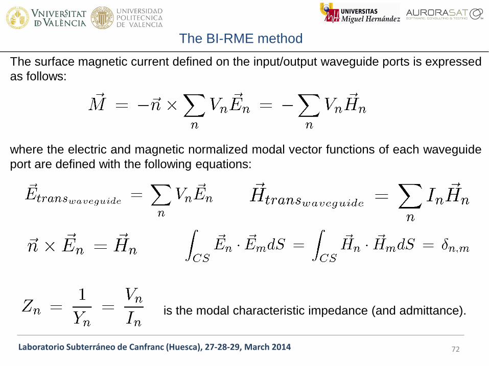
The surface magnetic current defined on the input/output waveguide ports is expressed as follows: where the electric and magnetic normalized modal vector functions of each waveguide port are defined with the following equations: is the modal characteristic impedance (and admittance).

Laboratorio Subterráneo de Canfranc (Huesca), 27-28-29, March 2014
The BI-RME method
73
- By imposing the boundary conditions of the tangential electromagnetic field on the surface of the metallic insets, as well as on the input/output waveguide ports, we can obtain the polar expansion of the generalized admittance matrix of the cavity:
where:
For the resonant modes computation

Laboratorio Subterráneo de Canfranc (Huesca), 27-28-29, March 2014
The BI-RME method
74

Laboratorio Subterráneo de Canfranc (Huesca), 27-28-29, March 2014
The BI-RME method
75
Laboratorio Subterráneo de Canfranc (Huesca), 27-28-29, March 2014
INDEX
76
• Introduction
• The rectangular waveguide
• The empty rectangular cavity
• Excitation of microwave cavities: coupling
• The BI-RME method
• Examples
• Conclusions
Laboratorio Subterráneo de Canfranc (Huesca), 27-28-29, March 2014 77
Examples
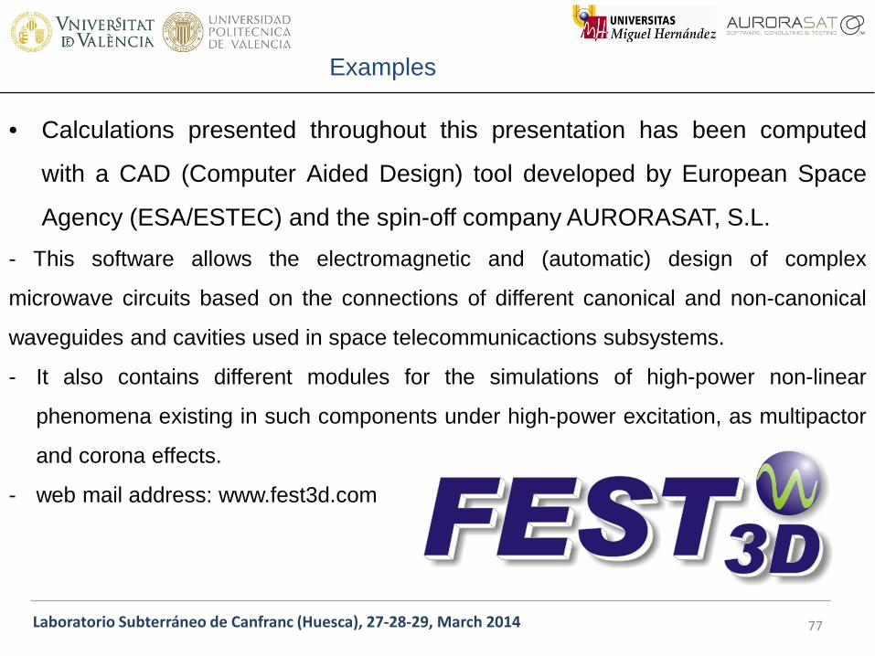
• Calculations presented throughout this presentation has been computed
with a CAD (Computer Aided Design) tool developed by European Space
Agency (ESA/ESTEC) and the spin-off company AURORASAT, S.L.
- This software allows the electromagnetic and (automatic) design of complex
microwave circuits based on the connections of different canonical and non-canonical
waveguides and cavities used in space telecommunicactions subsystems.
- It also contains different modules for the simulations of high-power non-linear
phenomena existing in such components under high-power excitation, as multipactor
and corona effects.
- web mail address: www.fest3d.com

Laboratorio Subterráneo de Canfranc (Huesca), 27-28-29, March 2014 78
Examples

Laboratorio Subterráneo de Canfranc (Huesca), 27-28-29, March 2014 79
Examples
• We are going to analyze the coupling between four different probes and a
rectangular cavity based on a standard WR-90 rectangular waveguide:
a = 22.86 mm, b = 10.16 mm, d = 1 m; conductivity of Cu at 20 C: σ = 5.96 .107 S/m
d
a
b
µ0, ε0
Laboratorio Subterráneo de Canfranc (Huesca), 27-28-29, March 2014 80
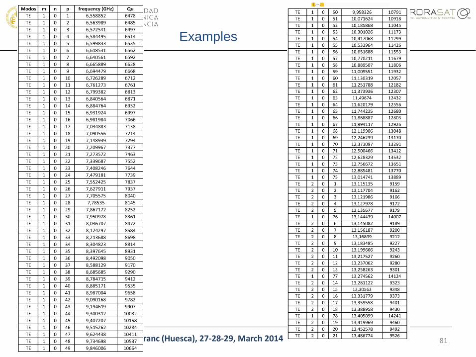
Examples
• This rectangular resonator supports 703 solenoidal modes in the frequency
range of the input coaxial waveguide:
Laboratorio Subterráneo de Canfranc (Huesca), 27-28-29, March 2014 81
Examples

Laboratorio Subterráneo de Canfranc (Huesca), 27-28-29, March 2014 82
Examples

Laboratorio Subterráneo de Canfranc (Huesca), 27-28-29, March 2014 83
Examples

Laboratorio Subterráneo de Canfranc (Huesca), 27-28-29, March 2014 84
Examples

Laboratorio Subterráneo de Canfranc (Huesca), 27-28-29, March 2014 85
Examples

Laboratorio Subterráneo de Canfranc (Huesca), 27-28-29, March 2014 86
Examples

Laboratorio Subterráneo de Canfranc (Huesca), 27-28-29, March 2014 87
Examples

Laboratorio Subterráneo de Canfranc (Huesca), 27-28-29, March 2014 88
Examples
• Example1: Simple electric probe exciting a rectangular cavity
WR-90: a=22.86 mm, b=10.16 mm
d = 1m b a

Laboratorio Subterráneo de Canfranc (Huesca), 27-28-29, March 2014 89
Examples
INPUT COAXIAL WAVEGUIDE: ri=0.635 mm, ro=2.11, εr=2.08; Z0=50 Ω
h=b/3=3.387 mm
b
2 ri
2 r0
h
d
d=λg/4=39.707 mm
βΤΕ10=2π/λg
βΤΕ10=((ω/c)2-(π/a) 2)1/2
ω=2π f
f = 10 GHz
Laboratorio Subterráneo de Canfranc (Huesca), 27-28-29, March 2014 90
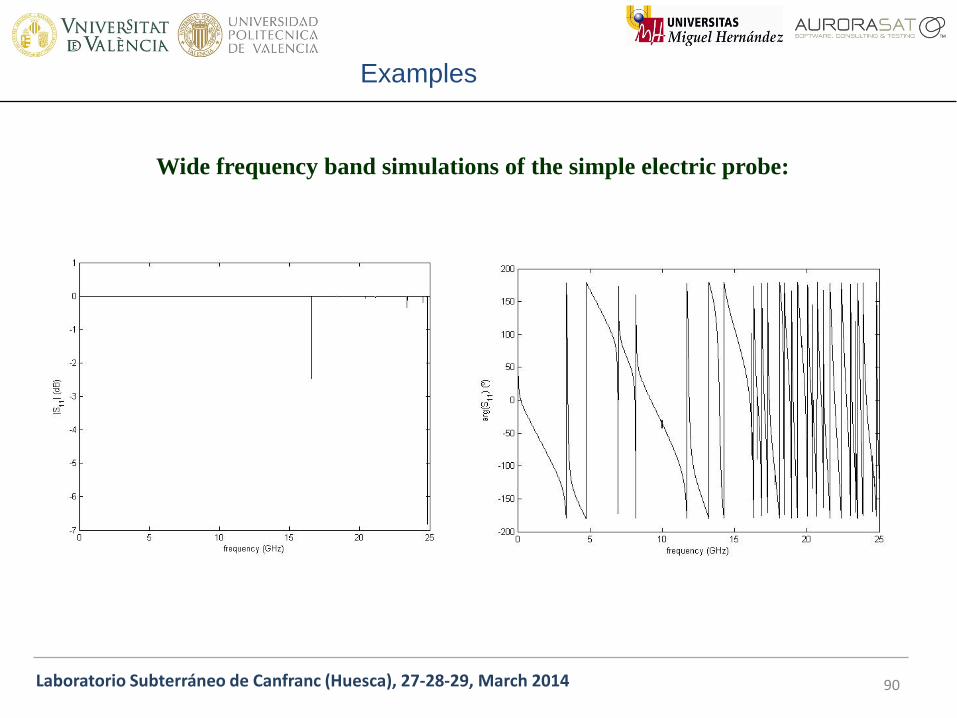
Examples
Wide frequency band simulations of the simple electric probe:

Laboratorio Subterráneo de Canfranc (Huesca), 27-28-29, March 2014 91
Examples
Identification of the most relevant ‘detected’ resonances of the simple electric probe:

Laboratorio Subterráneo de Canfranc (Huesca), 27-28-29, March 2014 92
Examples
Identification of the most relevant ‘detected’ resonances of the simple electric probe in the bandwidth of the rectangular waveguide (WR-90):

Laboratorio Subterráneo de Canfranc (Huesca), 27-28-29, March 2014 93
Examples
• Example2: Mushroom electric probe exciting a rectangular cavity
WR-90: a=22.86 mm, b=10.16 mm
d = 1m b a

Laboratorio Subterráneo de Canfranc (Huesca), 27-28-29, March 2014 94
Examples
INPUT COAXIAL WAVEGUIDE: ri=0.635 mm, ro=2.11, εr=2.08; Z0=50 Ω
2 ri
2 r0
b
h1
d
h2
2g
h1=h2=(b/3)/2=1.694 mm h=h1+h2=b/3=3.387mm
g=2ri=1.27 mm
d=λg/4=39.707 mm
βΤΕ10=2π/λg
βΤΕ10=((ω/c)2-(π/a) 2)1/2
ω=2π f
f = 10 GHz

Laboratorio Subterráneo de Canfranc (Huesca), 27-28-29, March 2014 95
Examples
Wide frequency band simulations of the mushroom electric probe:

Laboratorio Subterráneo de Canfranc (Huesca), 27-28-29, March 2014 96
Examples
Identification of the most relevant ‘detected’ resonances of the mushroom electric probe:
Laboratorio Subterráneo de Canfranc (Huesca), 27-28-29, March 2014 97
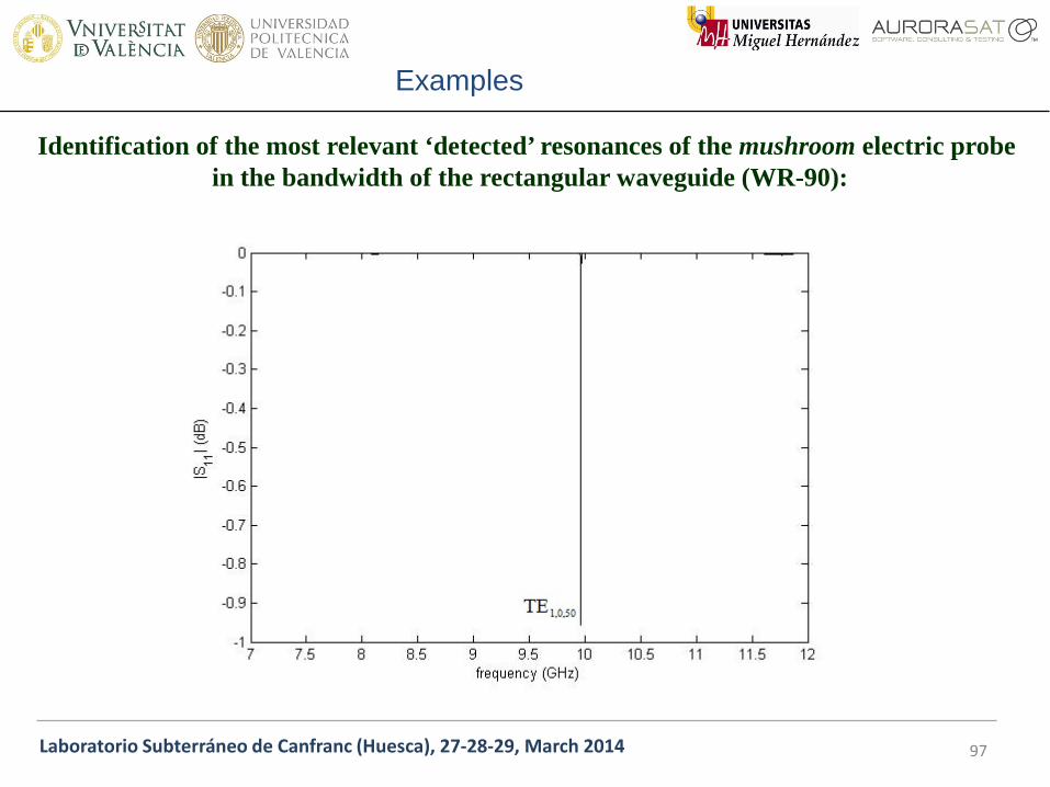
Examples
Identification of the most relevant ‘detected’ resonances of the mushroom electric probe in the bandwidth of the rectangular waveguide (WR-90):

Laboratorio Subterráneo de Canfranc (Huesca), 27-28-29, March 2014 98
Examples
• Example3: Vertical current loop exciting a rectangular cavity
a
WR-90: a=22.86 mm, b=10.16 mm
b d = 1m

Laboratorio Subterráneo de Canfranc (Huesca), 27-28-29, March 2014 99
Examples
INPUT COAXIAL WAVEGUIDE: ri=0.635 mm, ro=2.11, εr=2.08; Z0=50 Ω
2 ri
2 r0
60 mm
3 mm
b

Laboratorio Subterráneo de Canfranc (Huesca), 27-28-29, March 2014 100
Examples
Wide frequency band simulations of the vertical current loop:

Laboratorio Subterráneo de Canfranc (Huesca), 27-28-29, March 2014 101
Examples
Identification of the most relevant ‘detected’ resonances of the vertical current loop:
Laboratorio Subterráneo de Canfranc (Huesca), 27-28-29, March 2014 102
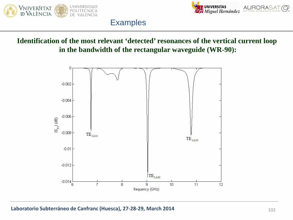
Examples
Identification of the most relevant ‘detected’ resonances of the vertical current loop in the bandwidth of the rectangular waveguide (WR-90):

Laboratorio Subterráneo de Canfranc (Huesca), 27-28-29, March 2014 103
Examples
• Example4: Horizontal current loop exciting a rectangular cavity
WR-90: a=22.86 mm, b=10.16 mm
d = 1m
a
b

Laboratorio Subterráneo de Canfranc (Huesca), 27-28-29, March 2014 104
Examples
INPUT COAXIAL WAVEGUIDE: ri=0.635 mm, ro=2.11, εr=2.08; Z0=50 Ω
2 ri
2 r0
50 mm
7 mm
a

Laboratorio Subterráneo de Canfranc (Huesca), 27-28-29, March 2014 105
Examples
Wide frequency band simulations of the horizontal current loop:

Laboratorio Subterráneo de Canfranc (Huesca), 27-28-29, March 2014 106
Examples
Identification of the most relevant ‘detected’ resonances of the horizontal current loop:
Laboratorio Subterráneo de Canfranc (Huesca), 27-28-29, March 2014 107
Examples
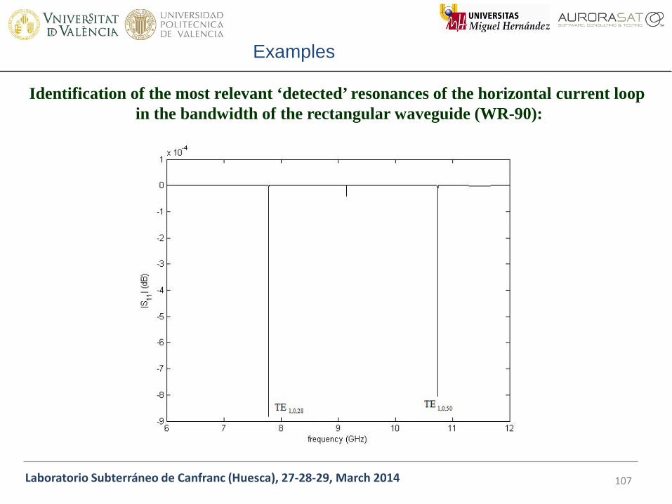
Identification of the most relevant ‘detected’ resonances of the horizontal current loop in the bandwidth of the rectangular waveguide (WR-90):

Laboratorio Subterráneo de Canfranc (Huesca), 27-28-29, March 2014 108
Examples
• Example5: Magnetic probe with vertical post exciting a rectangular cavity
WR-90: a=22.86 mm, b=10.16 mm
d = 1m
a
b

Laboratorio Subterráneo de Canfranc (Huesca), 27-28-29, March 2014 109
Examples
INPUT COAXIAL WAVEGUIDE: ri=0.635 mm, ro=2.11, εr=2.08; Z0=50 Ω
d
h=9.0 mm
g=1.5 mm
d=λg/4=39.707 mm
βΤΕ10=2π/λg
βΤΕ10=((ω/c)2-(π/a) 2)1/2
ω=2π f
f = 10 GHz
b 2 ri
2 r0
h
2g

Laboratorio Subterráneo de Canfranc (Huesca), 27-28-29, March 2014 110
Examples
Wide frequency band simulations of the magnetic probe with vertical post:

Laboratorio Subterráneo de Canfranc (Huesca), 27-28-29, March 2014 111
Examples
Identification of the most relevant ‘detected’ resonances of the magnetic probe with vertical post:

Laboratorio Subterráneo de Canfranc (Huesca), 27-28-29, March 2014 112
Examples
Identification of the most relevant ‘detected’ resonances of the magnetic probe with vertical post around the bandwidth of the rectangular waveguide (WR-90):
the electrical conducticity of the metallic walls has been modified

Laboratorio Subterráneo de Canfranc (Huesca), 27-28-29, March 2014
INDEX
113
• Introduction
• The rectangular waveguide
• The empty rectangular cavity
• Excitation of microwave cavities: coupling
• The BI-RME method
• Examples
• Conclusions

Laboratorio Subterráneo de Canfranc (Huesca), 27-28-29, March 2014 114
Conclusions
• We have presented and overview of rectangular waveguides and cavities,
presenting the most relevant relationships and concepts.
• A summary of the most important techniques to feed empty microwave
cavities has been summarized.
• BI-RME 3D formulation has been introduced, showing the most relevant
issues of the theory.
• Several coaxial probes have been explored for rectangular cavity
excitation.

Laboratorio Subterráneo de Canfranc (Huesca), 27-28-29, March 2014
Thanks a lot for your attention.
115
WE ARE OPEN TO COOPERATE WITH ALL OF YOU.


