1
EMPIRICAL ANALYSIS OF THE EFFECTIVENESS OF MONETARY
POLICY IN ZAMBIA
Peter Zgambo
Patrick M. Chileshe
Abstract
This study provides empirical analyses of the effectiveness of monetary policy in Zambia by
investigating the money demand function and the monetary transmission mechanisms (MTMs).
The money demand function is investigated using the Autoregressive Distributed Lag (ARDL)
approach while monetary transmission mechanisms are analysed through the Vector
Autoregressive (VAR) framework. The money demand function is found to be determined by real
income, the exchange rate and Treasury bill rates in the long-run while in addition to these
factors, inflation plays a role in the determination of money demand in the short-run. The money
demand function is also found to be stable, a result that points to the importance of monetary
aggregates in the conduct of monetary policy. As regards monetary transmission mechanisms,
the results found monetary aggregates (broad money) as being important in the transmission of
monetary policy while interest rates were found to have no significant effects on output and
prices. The exchange rate is also found to be an important channel for the transmission of
monetary policy. The key proposition from these results is that monetary aggregates will still
continue to play a role in the Bank of Zambia’s conduct of monetary policy even as the Bank
moves toward the adoption of inflation targeting, where the policy rate is envisaged to be the key
monetary policy tool.
JEL Classification Codes: E41, E49, E52
Key words: Monetary policy, money demand, monetary transmission mechanism
Prepared for the COMESA Monetary Institute
November 2014
2
Table of Contents
1.0 Introduction ............................................................................................................................... 3
2.0 Monetary Policy Implementation and Economic Performance in Zambia .......................... 5
3.0 Review of Monetary Policy Framework ................................................................................... 7
4.0 Literature Review on Money Demand and Monetary Transmission Mechanisms ................. 10
4.1 Theoretical Perspectives on the Demand for Money .......................................................... 10
4.2 Theoretical Perspectives on Monetary Policy Transmission Mechanisms ....................... 11
4.2.1 The Traditional Interest Rate Channel .......................................................................... 11
4.2.2 The credit channel ........................................................................................................ 12
4.2.3 The Exchange Rate Channel ......................................................................................... 13
4.2.4 The Asset Price Channel............................................................................................... 14
4.2.5 The Expectations Channel ............................................................................................ 15
5.0 Empirical Review.................................................................................................................... 16
5.1 Empirical Literature on the Demand for Money ................................................................. 16
5.2 Empirical Literature on Monetary Policy Transmission ..................................................... 17
6.0 Empirical Analysis .................................................................................................................. 19
6.1 Data ..................................................................................................................................... 19
6.2 Empirical Approach ............................................................................................................ 19
6.2.1 Empirical Model of the Money Demand Function ....................................................... 19
6.2.2 Econometric Approaches for Monetary Policy Transmission ...................................... 21
7.0 Results of the Estimated Models............................................................................................. 24
7.1 Unit Root and Co-integration Tests .................................................................................... 24
7.2 Estimated Results of the Money Demand Function ....................................................... 24
7.3 Estimated Results of the MTM ............................................................................................... 28
7.3.1 Interest Rate Pass-through ................................................................................................ 28
7.3.2 Estimated VAR Model of the MTM ................................................................................ 28
8.0 Conclusion and Policy Recommendations.............................................................................. 32
3
1.0 Introduction
The COMESA Committee of Central Bank Governors met at the 19th
Meeting in Lilongwe,
Malawi in November 2013 and considered a proposal from the Monetary and Exchange Rate
Policies Sub-Committee on the appropriate monetary policy regime for the COMESA region.
The proposal was in line with the regional block‘s continued efforts aimed at enhancing
monetary and financial integration in the region. The Governors welcomed the proposal, but
noted shortcomings such as the lack of sufficient empirical analysis to support the conclusions
contained in the proposal and inability to use recent information or data from member countries
to analyse specific country experiences of member countries. In light of these shortcomings, the
Governors directed the COMESA Monetary Institute (CMI) to undertake an in-depth empirical
assessment of the effectiveness of monetary policies in selected member countries. Zambia is
one such country identified for the study.
The conduct of monetary policies over the last two decades in most countries in the COMESA
region have been based on the monetary aggregate targeting (MAT) framework1. The MAT
framework is premised on the existence of a strong and stable relationship between monetary
aggregates (broad money) and the ultimate monetary policy goals, inflation or output. In Zambia,
monetary policy conduct was exclusively based on the MAT framework from the early 1990s to
March 2012. During this period, monetary policy in Zambia helped to reduce inflation from the
triple digits of the 1990s to current single digits. Other member countries in the COMESA region
using the similar framework have also managed to lower inflation from higher levels to relatively
lower levels in recent times.
An assessment of the performance of monetary policy in Zambia under the MAT framework
suggests that monetary policy has been effective, judging from the reduction in inflation rates
from triple digits of the early 1990s to current single digits. However, firm conclusions about the
effectiveness of monetary policy can only be deduced through a detailed empirical analysis that
takes account of the underlying relationships between the monetary policy framework and
monetary policy goals or objectives and outcomes. Such an analysis may also shed light on the
motivation behind the Bank of Zambia‘s recent move to consider alternative monetary policy
frameworks for the conduct of monetary policy.
Hence, the main objective of this study is to empirically assess the effectiveness of monetary
policy in the COMESA region, with particular reference to Zambia. This is accomplished
through the empirical examination of the money demand function and empirical analysis of the
monetary transmission mechanisms. The rationale behind the adopted approach is to assess
whether the money demand function exhibits the characteristics required for the success of
monetary policy under a MAT framework as well as to assess the channels through which
monetary policy is transmitted under such a framework. Based on the empirical findings, the
study makes recommendations for an appropriate monetary policy regime that can be
implemented in Zambia, and by extension in the COMESA region over the medium to long-
term.
1Other COMESA member countries that at least used the MAT framework at one time include Kenya, Uganda,
Rwanda, Burundi, Egypt, Mauritius, Madagascar and Zimbabwe.
4
The results from the empirical analysis of the money demand function suggest that in the long-
run, demand for real money balances is determined by real income and opportunity cost
variables (exchange rate and the Treasury bill rate). As regards the exchange rate, the negative
and significant coefficient associated with the exchange rate demonstrates the presence of
currency substitution in the estimated money demand function for Zambia. This result is not
surprising given that residents are free to hold foreign currency-denominated accounts and may
use such accounts to hedge the risks associated with inflation or the depreciation of the exchange
rate. In the short-run, money demand is found to be significantly influenced by the exchange
rate, short-term interest rates, inflation, and income dynamics. In terms of stability, the money
demand function is found to be generally stable.
As regards the monetary transmission mechanisms, empirical evidence from this study suggests
that the MTM is generally weak and more closely connected to monetary aggregates (broad
money) than interest rates. In this regard, the money channel appears to be one of the important
channels through which monetary policy is transmitted in Zambia, given its significant impact on
output or inflation, in contrast to interest rates. Evidence also shows the importance of the
exchange rate channel in monetary policy transmission in Zambia given the instantaneous
response of the exchange rate following a monetary expansion. However, results from the
interest rate pass-through suggest that market interest rates appear to be gaining in importance
though their effect of output or prices remain insignificant.
The overall recommendation from this study is that as the process of modernising monetary
policy framework, it is clear that in the case of Zambia monetary aggregates will still continue to
play a role in monetary policy conduct. In this regard, it would be premature to abandon the
traditional policy focus on monetary aggregates, given their influence on the key macroeconomic
outcomes of output and prices. A key implication from this study is therefore that monetary
policy in Zambia, and other COMESA member countries, should continue to consider
developments in monetary aggregates while gradually transitioning to modern monetary policy
frameworks. In addition, measures should be put in place that are aimed at enhancing monetary
transmission mechanisms, particularly the interest rate channel, by promoting financial
deepening and economic development more generally.
The paper is structured as follows: Section 2 discusses monetary policy implementation and
economic performance in Zambia while the monetary policy framework is reviewed in Section 3.
Theoretical literature review on the money demand function and monetary transmission
mechanisms is presented in Section 4; empirical literature review on the money demand function
and monetary transmission mechanisms is provided in Section 5. The empirical approaches used
in the study are presented in Section 6 while Section 7 discusses the results of the estimated
models. The paper ends with concluding remarks and recommendations in Section 8.
5
2.0 Monetary Policy Implementation and Economic Performance in Zambia
Prior to the 1990s, the conduct of monetary policy in Zambia was driven by multiple objectives,
which included the provision of cheap credit mainly to state owned enterprises and promotion of
economic growth through various initiatives and incentives. In addition, monetary policy was
used to finance the government‘s budget through borrowing from the central bank.
During this period, monetary policy relied mainly on the use of direct instruments such as
interest rate controls, directed credit allocation as well as core liquid assets and statutory reserve
ratios. Reliance on direct monetary policy instruments was partly based on the prevailing
economic paradigm which was dominated by the state, and the realisation by the central bank
that it had little control over money supply since the banking sector was dominated by foreign
banks that tended to issue loans to mostly foreign owned companies without regard to prevailing
economic and financial conditions (Kalyalya, 2001).
Partly due to monetary policy‘s lack of clear focus, macroeconomic conditions deteriorated
steadily during the period prior to the 1990s.The persistent use of the central bank to finance
fiscal deficits as well as failure of the monetary authority to control money supply resulted in
rising inflation (Bigstern and Mugerwa, 2000). The growing economic problems were
compounded by internal and external imbalances as well as structural and institutional
deficiencies. Domestically, price controls on most food items, widespread consumer subsidies,
and the industrialisation strategy of import substitution coupled with weak public administration
worsened the fiscal position and led to a highly inefficient allocation of resources. Externally, the
country‘s balance of payment position became unsustainable following the loss of international
reserves due to growing foreign debt servicing and dwindling export earnings resulting from
falling copper prices and production volumes.
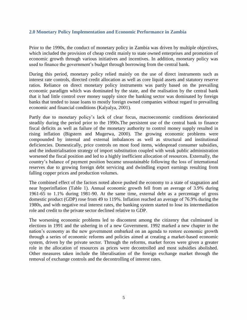
The combined effect of the factors noted above pushed the economy to a state of stagnation and
near hyperinflation (Table 1). Annual economic growth fell from an average of 3.9% during
1961-65 to 1.1% during 1981-90. At the same time, external debt as a percentage of gross
domestic product (GDP) rose from 49 to 119%. Inflation reached an average of 76.9% during the
1980s, and with negative real interest rates, the banking system started to lose its intermediation
role and credit to the private sector declined relative to GDP.
The worsening economic problems led to discontent among the citizenry that culminated in
elections in 1991 and the ushering in of a new Government. 1992 marked a new chapter in the
nation‘s economy as the new government embarked on an agenda to restore economic growth
through a series of economic reforms and policies aimed at creating a market-based economic
system, driven by the private sector. Through the reforms, market forces were given a greater
role in the allocation of resources as prices were decontrolled and most subsidies abolished.
Other measures taken include the liberalisation of the foreign exchange market through the
removal of exchange controls and the decontrolling of interest rates.
6
Table 1: Evolution of Key Monetary and Economic Variables
Source: World Bank Database, and BoZ database. (Real Interest Rate is the lending interest rate adjusted
for inflation as measured by the GDP deflator.)
Changes in the economic environment carried through to the conduct of monetary policy. The
Bank of Zambia (BoZ) Act was amended in 1996, narrowing the central bank‘s objective to price
and financial system stability. Consequently, monetary policy concentrated on creating a stable
macroeconomic environment to support sustainable economic growth. The resultant institutional
arrangement following the amendment of the BoZ Act was that the Bank was empowered to
pursue appropriate monetary policy in support of sustainable economic growth. The inflation
target was to be set by the Ministry of Finance in consultation with the Bank of Zambia. Once
the inflation target has been set, BoZ had discretion to use monetary policy instruments at its
disposal in managing liquidity conditions with the aim of achieving the inflation target. Under
the new framework, BoZ started to target monetary aggregates, an approach premised on a
strong and stable relationship between the ultimate target (inflation) and money supply.
The Bank also started to rely on indirect market-based monetary policy instruments in the
conduct of monetary policy. These instruments included primary auctions of treasury bills and
government bonds, as well as auctions of short-term credit and term deposits under open market
operations (OMO). In addition, the Bank can use purchases and sales of foreign exchange as a
tool of monetary policy as well as management of exchange rate policy. With these indirect
instruments, the BoZ tried to influence the behavior of financial institutions and other market
players through market mechanisms. This helped improve control of money supply and inflation
and also promoted a more efficient allocation of credit and financial market development in
general.
The change in the monetary policy framework and its implementation contributed to a marked
improvement in Zambia‘s macroeconomic environment. Money growth and inflation declined
sharply, with the latter being held in the single digits since 2006.The liberalization of lending and
deposit rates initially caused real interest rates to spike, but they subsequently stabilised at about
5%. Moreover, real GDP growth steadily increased to an average of 6.6% during the period 2001
to 2012 from an average of 0.8% during 1991 to 2000 (see Table 1 above).
Indicator Name 1961-1970 1971-1980 1981-1990 1991-2000 2001-2010 2011 2012
Real Per Capita GDP Growth (annual % growth) 0.8 -1.9 -1.8 -1.7 2.8 3.6 4.0
Real GDP Growth (annual % growth) 3.9 1.5 1.1 0.8 5.6 6.8 7.3
Average Annual Inflation Rate - 11.1 76.9 68.1 15.5 6.4 6.6
External Debt Stocks (% of GNI) - 75.3 206.1 214.3 89.9 27.4 27.6
External Debt(% of GDP) - 48.7 119.3 147.3 67.9 18.1 19.0
Total Debt Service (% of exports ) 2.9 26.2 25.1 25.0 12.9 2.2 2.2
Total Reserves (% of total external debt) - 10.1 2.8 2.8 23.1 47.0 56.5
Total Reserves (% of GDP) 18.6 7.1 4.5 5.0 9.1 12.1 14.7
Broad Money (% of GDP) 19.3 29.0 30.9 18.2 21.3 23.4 24.1
Broad Money Growth (annual % growth) 27.2 10.5 41.5 49.9 22.7 21.7 17.9
Real Interest Rate (%) - 0.8 -15.5 3.1 11.3 5.6 5.6
Domestic Credit (% of GDP) -0.3 41.9 63.9 59.6 28.2 18.1 18.5
Domestic Credit to Private Sector (% of GDP) 8.5 17.1 14.0 7.5 9.6 12.3 14.8
External Balance (% of GDP) 15.1 0.9 -1.7 -6.9 -2.4 9.0 -
7
3.0 Review of Monetary Policy Framework
The MAT framework employed by Bank of Zambia to conduct monetary policy is based on the
existence of a strong and predictable relationship between monetary aggregates and the ultimate
monetary policy target, inflation. Literature developed around the role of money in monetary
policy suggests that money can be useful in the conduct of monetary policy if it is used as an
―information variable‖ and or as a monetary policy instrument or target. In this regard, money is
useful as an information variable ―if fluctuations in money provide relevant information about
the current or future fluctuations in key macroeconomic variables that monetary policy seeks to
influence…while as a target or policy instrument, money is useful if a given rate of growth in
money is consistent with the desired level of inflation or output‘s rate of growth‖ (Friedman and
Kuttner, 1982). From the foregoing, it should be noted that for money to be useful as an
information variable, it must provide important and systematic information about the future paths
of key variables for monetary policy. Similarly, for money to be useful as a monetary policy
target or instrument, it must have some relation with key macroeconomic variables such as
inflation or output. The implication of this is that for a monetary policy framework based on
money to be successful, there has to be a strong and reliable relationship between the monetary
aggregate selected as the target or instrument and the ultimate target, which could be inflation or
output.
In the case of Zambia, base money or reserve money has been used as the operational target in
the conduct of monetary policy while broad money has been used as the intermediate target with
inflation being the ultimate target. Reserve money represents the liability of the central bank, and
its choice as the operational target is premised on the central bank‘s ability to control this
liability. Reserve money is in turn linked to broad money through the money multiplier, which is
assumed to be stable and predictable. In this regard, if the money multiplier is stable and
predictable, the central bank could control the overall monetary conditions in the economy by
keeping reserve money at a level that is consistent with desired broad money growth. The desired
expansion of broad money should in turn be consistent with the inflation target.
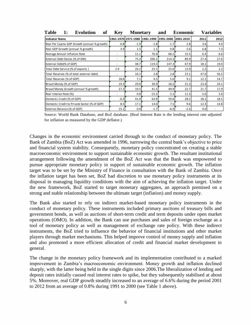
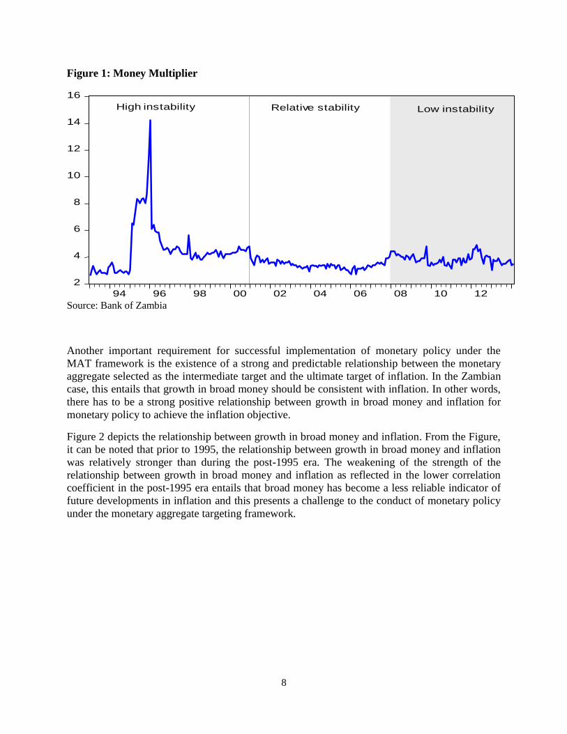
A review of the money multiplier for Zambia depicted in the Figure 1 suggests that the money
multiplier has not been particularly stable during the period of the MAT framework. Prior to
2000, the economy was characterized by general instability with relatively high growth rates in
money supply and high inflation rates. This is partly reflected in the relatively high instability of
the money multiplier. However, from about 2001 to around 2007, the money multiplier exhibits
some relative stability. From around 2008 to the end of the sample period (February 2014), the
stability of the money multiplier seems to be questionable.
8
Figure 1: Money Multiplier
2
4
6
8
10
12
14
16
94 96 98 00 02 04 06 08 10 12
High instability Relative stability Low instability
Source: Bank of Zambia
Another important requirement for successful implementation of monetary policy under the
MAT framework is the existence of a strong and predictable relationship between the monetary
aggregate selected as the intermediate target and the ultimate target of inflation. In the Zambian
case, this entails that growth in broad money should be consistent with inflation. In other words,
there has to be a strong positive relationship between growth in broad money and inflation for
monetary policy to achieve the inflation objective.
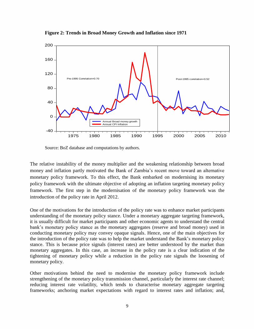
Figure 2 depicts the relationship between growth in broad money and inflation. From the Figure,
it can be noted that prior to 1995, the relationship between growth in broad money and inflation
was relatively stronger than during the post-1995 era. The weakening of the strength of the
relationship between growth in broad money and inflation as reflected in the lower correlation
coefficient in the post-1995 era entails that broad money has become a less reliable indicator of
future developments in inflation and this presents a challenge to the conduct of monetary policy
under the monetary aggregate targeting framework.
9
Figure 2: Trends in Broad Money Growth and Inflation since 1971
-40
0
40
80
120
160
200
1975 1980 1985 1990 1995 2000 2005 2010
Annual Broad money growth
Annual CPI Inflation
Post-1995 correlation=0.52Pre-1995 Correlation=0.70
Source: BoZ database and computations by authors.
The relative instability of the money multiplier and the weakening relationship between broad
money and inflation partly motivated the Bank of Zambia‘s recent move toward an alternative
monetary policy framework. To this effect, the Bank embarked on modernising its monetary
policy framework with the ultimate objective of adopting an inflation targeting monetary policy
framework. The first step in the modernisation of the monetary policy framework was the
introduction of the policy rate in April 2012.
One of the motivations for the introduction of the policy rate was to enhance market participants
understanding of the monetary policy stance. Under a monetary aggregate targeting framework,
it is usually difficult for market participants and other economic agents to understand the central
bank‘s monetary policy stance as the monetary aggregates (reserve and broad money) used in
conducting monetary policy may convey opaque signals. Hence, one of the main objectives for
the introduction of the policy rate was to help the market understand the Bank‘s monetary policy
stance. This is because price signals (interest rates) are better understood by the market than
monetary aggregates. In this case, an increase in the policy rate is a clear indication of the
tightening of monetary policy while a reduction in the policy rate signals the loosening of
monetary policy.
Other motivations behind the need to modernise the monetary policy framework include
strengthening of the monetary policy transmission channel, particularly the interest rate channel;
reducing interest rate volatility, which tends to characterise monetary aggregate targeting
frameworks; anchoring market expectations with regard to interest rates and inflation; and,
10
promoting transparency in the way banks set the lending rates by making the policy rate the
reference rate for pricing of credit products.
However, it should be noted that despite the weakening of the relationship between broad money
and inflation, relative money multiplier instability and the need to modernise the monetary policy
framework, monetary aggregates will continue to play a role in the conduct of monetary policy in
Zambia.
4.0 Literature Review on Money Demand and Monetary Transmission Mechanisms
4.1 Theoretical Perspectives on the Demand for Money
There are a number of theories on the demand for money. In the classical tradition, cash balances
are held primarily to undertake transactions, and therefore depend on the level of income.
However, this position was changed in the 1930s when Keynes postulated three motives for
holding real money balances: transactions; precautionary; and speculative demand for money.
Transactions and precautionary motives of the demand for real money balances follow the
classical tradition in that it depends on the level of income while the speculative demand for
money departs from the classical tradition by arguing that the demand for real money balances
depend on the interest rates. Following Keynes liquidity preference theory, several authors have
offered criticisms regarding Keynes rationale for a speculative demand for money and have
contributed to the theoretical literature by distinguishing broadly between the transactions
demand (Baumol, 1952; Tobin, 1956) and the asset motive (Tobin, 1956; Friedman, 1956). In
general, all available theories portray that the demand for money depends positively on the real
GDP and the price level due to the transactions motive while it is negatively related to interest
rates due to the speculative motive as shown below;
( ( ) ( ) ( ))
In real terms, the money demand function is often denoted as;
( )
Equation (2) is viewed as the liquidity preference and represents the desired level or long run real
money demand function and assumes a unit elasticity of the nominal cash balances with respect
to the price level. The unitary elasticity of the demand for money portrays the common argument
in the monetarist literature that ―inflation is everywhere and always a monetary phenomenon in
the long-run‖ (Friedman, 1968). In this regard, monetary policy will only be effective in
controlling inflation if there is a stable money demand function in the long-run. If money
demand is stable, changes in money supply are closely related to prices and income, and hence it
is possible for the central bank to control inflation through appropriate changes to money supply.
On the other hand, if the demand for money function is unstable, changes in money supply are
11
not closely related to prices and income and it becomes difficult to control inflation using
adjustments in money supply.
4.2 Theoretical Perspectives on Monetary Policy Transmission Mechanisms
Monetary policy transmission is a process through which central bank actions are transmitted to
real sector variables of inflation, output and employment (Taylor, 1995). Although the long-run
neutrality of money view of the classical tradition is widely accepted, monetary policy is at least
assumed to affect real variables in the short-run due to the Keynesian view of nominal sticky
prices or due to wealth, income, liquidity and expectations effects (Dabla-Norris and
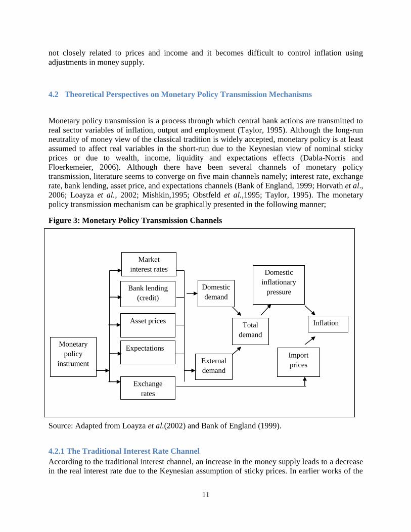
Floerkemeier, 2006). Although there have been several channels of monetary policy
transmission, literature seems to converge on five main channels namely; interest rate, exchange
rate, bank lending, asset price, and expectations channels (Bank of England, 1999; Horvath et al.,
2006; Loayza et al., 2002; Mishkin,1995; Obstfeld et al.,1995; Taylor, 1995). The monetary
policy transmission mechanism can be graphically presented in the following manner;
Figure 3: Monetary Policy Transmission Channels
Source: Adapted from Loayza et al.(2002) and Bank of England (1999).
4.2.1 The Traditional Interest Rate Channel
According to the traditional interest channel, an increase in the money supply leads to a decrease
in the real interest rate due to the Keynesian assumption of sticky prices. In earlier works of the
Monetary
policy
instrument
Market
interest rates
Bank lending
(credit)
Asset prices
Exchange
rates
Domestic
demand
External
demand
Total
demand
Domestic
inflationary
pressure
Import
prices
Inflation
Expectations
12
Keynesian approach, this channel was thought to mainly operate through the investment channel
but later theoretical and research works recognised that consumers‘ decisions about real estate
and durable expenditure (spending on cars, own house construction and other durable goods) are
also influenced by the real interest rate (Mishkin, 1995). Changes in the real interest rates induce
economic agents to change their investment and consumption expenditure and thereby changing
economic activity. This channel implicitly assumes that the central bank is able to influence
long-term real interest rates through manipulation of short-term real interest rates. Mishkin
(1995) notes that this suggests the expectation hypothesis of the term structure of interest rates
holds true. The expectation hypothesis of the term structure states that the long-term interest rate
is an average of expected future short-term interest rates, suggesting that lower real short-term
interest rate leads to a fall in the real long-term interest rate. Ozsuca (2009) also notes that
theoretically the interest rate channel also circumvent the zero interest bound. Expansionary
monetary policy increases expected prices of goods and services and therefore lowers real
interest rates, hence lower interest rates stimulates consumer spending. The Interest rate channel
is often referred to as the hallmark of the ―Money View‖.
4.2.2 The credit channel
The credit channel came into being as a result of dissatisfaction over the effects of monetary
policy explained through interest rate effects on durables expenditure and investment. The credit
channel explains the impact of monetary policy via the effects of informational asymmetry
between the lender and the borrower (Mishkin, 1995). The credit view proposes that as a result
of these informational asymmetries, two channels of monetary transmission arise: those that
operate through the effects on bank lending as well those that affect the firms‘ and households
balance sheets. The bank lending channel is based on the assumption that financial
intermediaries are best suited to solve problems of informational asymmetry in credit markets
while the balance sheet channel is based on the effects of monetary policy on the net worth of
firms and hence their collateral (Simatele, 2004).
The bank lending channel operates through the quantity of loans supplied by the commercial
banks to firms and households. As Dabla-Norris and Floerkemeier (2006) notes ―The bank
lending channel operates via the influence of monetary policy on the supply of bank loans, that
is, the quantity rather than the price of credit‖. An expansionary monetary policy increases
excess reserves in the banking system. This makes loans available to bank dependent economic
agents to increase. Increased supply of loans makes it possible for bank dependent economic
agents to increase investment as well as consumption spending which result in increased
economic activity. This channel is likely to be more effective in economies where there are many
small firms with little capacity to raise capital on stock markets. Further, an under-developed
capital markets as is the case in most developing or underdeveloped economies makes the bank
lending channel stronger.
Due to asymmetric information in financial markets, the role played by commercial banks as
financial intermediaries becomes important and thus comes in the balance sheet channel (Tahir,
2012). Existence of asymmetric information gives rise to moral hazard and adverse selection. As
Mishkin (1995), Tahir, (2012) and Bernanke and Gertler (1995) emphasis that banks have a
comparative advantage in assessing the balance sheets of borrowers and hence help in mitigating
adverse selection as well as moral hazard. Under the balance sheet channel, there are several
13
ways through which monetary policy affect the balance sheets of economic agents and hence the
occurrence of moral hazard and adverse selection.
Expansionary monetary policy affects the net-worth of firm through an increase in stock prices
as described earlier. Further, expansionary monetary policy which reduces interest rates reduces
the debt servicing burden of firms and households. This improves the cash flow of firms and
thereby enhances their chance of accessing loans from banks. The improvement in the balance
sheets of households and firms due to expansionary policy reduces the possibility of moral
hazard and adverse selection. All this brings about an increase in borrowing resulting in
increased consumer spending and investment, and consequently economic activity. It is
important to emphasise here that all the other channels operate mostly through the credit channel.
4.2.3 The Exchange Rate Channel
The exchange rate channel is one of the primary transmission channels of monetary policy in
open economies, especially those with flexible exchange rate regimes. Monetary policy can
influence the exchange rate through interest rates (the popular uncovered interest rate parity
condition), direct intervention in foreign exchange markets or through inflationary expectations
(Dabla-Norris et al., 2006). In this channel, monetary policy affects economic activity (output)
through net exports.
This link between monetary policy and exchange rate under the uncovered interest parity (UIP)
condition were popularised by the open macroeconomic models developed independently by
Fleming (1962), Mundell (1963), and Dornbusch (1976). Under the UIP assumptions, the
difference between interest on domestic financial assets and foreign assets is equal to the
expected change in exchange rates. The change in exchange rate as a result of monetary policy
action in these models affects both aggregate demand and aggregate supply. On the demand side,
expansionary monetary policy which reduces interest rates makes the local currency to
depreciate as investors divest from the local market to invest in foreign markets. The real
depreciation of the currency makes the country‘s exports cheaper compared to foreign produced
goods. This results into an increase in the net exports and hence stronger aggregate demand
leading to an increase in output (Obsfeld and Rogoff, 1996; Taylor, 1993; Mishkin (1995, 2001);
Loazya and Schmidt-Hebbel, 2002). However, on the supply side a real depreciation of the
currency raises the domestic prices of imported goods, which directly increases domestic
inflationary pressure through the so-called exchange rate pass through (Ozdogan, 2009; Loazya
and Schmidt-Hebbel, 2002; Alper 2003; Campa and Goldberg, 2004; Kara et al., 2005).
Moreover, the higher prices of imported inputs contracts output and increases prices (Loazya and
Schmidt-Hebbel, 2002). The extent of the exchange pass-through to domestic price, hence
overall inflation, depends on the level of the country‘s dependence on imported consumer and
intermediate goods, the magnitude and timing of the appreciation, as well as macroeconomic
environmental (Alper, 2003; Campa and Goldberg, 2004; Kara et al., 2005).
The exchange rate channel also operates through the effect of monetary policy on the
international competitiveness of exports and import competing goods (Dabla-Norris and
Floerkermeier, 2006). Expansionary monetary policy which lowers interest rates leads to a real
currency depreciation making domestically produced exports cheaper on international markets
resulting in increased demand for them and more output and vice versa. Furthermore, the effects
14
of monetary policy on the exchange rate may exert significant effect on the balance sheets of
households and firms which change the net-worth and debt-service ratio. These changes affect
the borrowing and spending patterns of economic agents, especially for highly dollarized
countries (Dabla-Norris and Floerkermeier, 2006; Kamin et al., 1998).
The strength of the exchange rate channel is affected by several factors such as the exchange rate
regime, sensitivity of the interest rates, the size and openness of the economy, degree of capital
mobility and the degree of expenditure switching between domestic and imported goods (Boivin
et al., 2010;Mishra et al.,2010; Tahir, 2012).
4.2.4 The Asset Price Channel
Monetary policy affects asset prices such as bonds, equity and real estate, changing firms‘ stock
market values and household wealth. Changes in stock market values and household wealth in
turn affect aggregate demand. The asset price channel of monetary policy transmission is
assumed to operate through two mechanisms namely; the Tobin‘s (1969) Q-theory of investment
and Ando-Modigliani (1963) life cycle theory of consumption. Although monetarists and
Keynesians arrive at the same conclusion of how these views work, they disagree on how
monetary policy affects equity prices (Afandi, 2005). The Keynesians argue that the fall in
interest rates following monetary expansion makes bonds less attractive to investors relative to
equities, thereby making the prices of equities to increase and vice versa. On the other hand, the
monetarists believe that expansionary monetary policy affects equity prices through an increase
in the demand for equities as economic agents find themselves with excess liquidity which they
can use to invest in equities, given their short-run supply, prices increase (Mishkin, 1995).
The asset price channel that works through the Tobin‘s Q (1969) theory of investment relies on
the effect of monetary induced changes in equity prices on the Tobin‘s Q. James Tobin (1969)
defined the Q as the ratio of the market value of a firm to the replacement cost of capital owned
by that firm. This ratio is a summary measure of one important impact of financial markets on
purchases of goods and services (Afandi, 2005). Tobin (1969) argues that although in
equilibrium the Q has a normal value equal to one, which sustains capital replacement and
expansion at the natural rate of economic growth, in reality the Q often exceeds one by the
capitalised value of monopoly profits and rents. In the short-run, the Q changes as a result of
random events, policies and expectations which create or destroy incentives for capital
investment. Amongst these is monetary policy.
Thus, the Tobin‘s view of the asset channel works as follows. Expansionary monetary policy
increases the demand for equities (either by the Keynesian or Monetarist argument), raising
equity prices and thereby boost market value of firms relative to the replacement cost of capital.
This will result in increased investment and therefore output. Furthermore, higher equity prices
also raise the net-worth of firms and households and hence improve their credit worthiness and
access to funds, the effects of which would partly reflect the balance sheet channel of monetary
policy (Afandi, 2005).
On the other hand, in the Ando-Modigliani life cycle model of consumption monetary policy
changes affect the economic agents‘ long-term wealth and therefore, alters their consumption
pattern. The basic premise of Ando-Modigliani theory is that consumers smooth out their
consumption over time and this consumption depends on lifetime resources and not only current
consumption (Mishkin, 1995). Expansionary monetary policy which lowers interest rates
15
changes consumers‘ portfolio composition in accordance with the risk of each asset class. In this
case, a decrease in the interest rates encourages people to reduce their holding of interest earning
deposits and bonds and substitute them with equity/stocks, thereby increasing stock prices
(Afandi, 2005). Given that a major component of wealth is in common stocks, the increase in
stock prices increases their wealth resulting in higher consumption expenditure and hence output.
Although Tobin‘s Q theory of investment and Ando-Modigliani assume that monetary policy
affects the prices of stocks and bonds, Meltzer (1995) takes a wider view of the impact of
monetary policy on various asset prices. He contends that the short-term nominal interest rate is
not the only mechanism affected directly by monetary policies. Monetary policy actions affect
the markets for durable goods, real estate, equities, and financial assets along with interest rates.
Changes in all of these asset prices affect aggregate demand and output.
Tahir (2012) notes the following factors as the key determinants of the asset price channel: the
participation of households in the capital market; the generation of funds by firms through
issuance of shares; and the level of development of the national stock market. This is confirmed
by Kamin et al. (1998) and Butkiewicz and Ozgdogan (2008) who notes that the asset price
channel in developing and emerging markets is weak and more unpredictable compared to
developed economies due to shallower and uncompetitive markets as well as highly unstable
macroeconomic environments.
4.2.5 The Expectations Channel
Since the early years of modern macroeconomics, expectations have been acknowledged to
influence the behaviour of economic agents. For example, Keynes (1936) in his General Theory
comments ―…the behaviour of each individual firm in deciding its daily output will be
determined by its short-term expectations — expectations as to the cost of output on various
possible scales and expectations as to the sale-proceeds of this output; though, in the case of
additions to capital equipment and even of sales to distributors, these short-term expectations
will largely depend on the long-term (or medium-term) expectations of other parties‖.
Economists generally agree that expectations are important in influencing economic activity, but
they differ on how these expectations are generated. Friedman and other monetarists, postulate
adaptive expectations while the new classical school lead by Lucas and the New Keynesian
School argue for rational expectations.
Since economic agents are forward looking and rational, the expectation channel is in effect
fundamental to the working of all channels of monetary policy transmission. Empirically, this
channel is mainly operational in developed economies with well-functioning and deep financial
markets (Davoodi et al., 2013). For example, if economic agents expect future changes in the
policy rate, this can immediately affect medium and long-term interest rates. Further, monetary
policy can be used to influence expectations of future inflation and thus influence price
developments. Inflation expectations matter in two important areas. First, they influence the level
of the real interest rate and thus determine the impact of any specific nominal interest rate.
Second, they influence price and money wage-setting behaviour and feed through into actual
inflation in subsequent periods. Similarly, changes in the monetary policy stance can influence
expectations about the future course of real economic activities by affecting inflationary
expectations and the ex-ante real interest rate and guiding the future course of economic
activities.
16
5.0 Empirical Review
5.1 Empirical Literature on the Demand for Money
Empirical literature on the money demand function has been in existence for long time,
elsewhere. However, in the sub-Saharan Africa region empirical studies on the demand for
money started to emerge following significant economic reforms undertaken in these countries
focusing on establishing the impact of the financial sector reforms on the stability of the money
demand function. Generally, it is argued that economic reforms especially those focusing on the
financial sector have significant impact on the money demand function with important
consequences for monetary policy effectiveness under a monetary targeting framework.
In a monetary aggregate policy framework, the stability of the demand for money function is
crucial for the for monetary policy formulation. This is because it enables a policy driven change
in a monetary aggregate to have a forecastable influence on aggregate demand, interest rates and
prices (Sriram, 1999). Thus, any reforms with fundamental impact on money demand will affect
the effectiveness of monetary policy. In this regard, a number of studies have been done to
ascertain the impact of financial reforms on the stability of the demand function with varied
results; a few of these studies are reviewed.
Ogunsakin and Awe (2014) investigates the impact of financial sector reforms on the stability of
the money demand function in Nigeria. They estimate a parsimonious error correction model
(ECM) which include real broad money balances; inflation; exchange rate; foreign interest rates;
savings deposit rate; treasury bill, and a dummy for post-liberalisation era. They find that the
significant determinants for money demand in Nigeria are inflation, foreign interest rates,
Treasury bill rate, savings deposit rate and real GDP. A test for the stability shows that the
demand for money function remained stable despite the reforms, implying using of monetary
targets is still relevant.
Dagher and Kovanen (2011) analyses the stability of the money demand function in Ghana using
bounds testing procedure developed by Pesaren (2001). They estimate an Auto-Regressive
Distributive Lag (ARDL) model which includes changes in broad money, its own lags, current
and lagged values of the explanatory variables. The explanatory variables include income,
exchange rate, deposit rate, TB rate, US TB rate, and the US libor rate. They find that the TB
rate, US TB rate and the Libor rate have no significant impact on the demand while income and
exchange rate were found to have significant effects. Specifically, they find that a depreciation
increases money demand as is the increase in incomes. Furthermore, they find a faster
convergence of the ECM to equilibrium once there is a misalignment. Using a CUSUM and
CUSUM squares test on the residuals of the ECM model they find that the money demand is
stable.
Lungu et al. (2012) examines the behaviour of the demand for money in Malawi for the period
1985 to 2010. Specifically, they seek to tackle two objectives: i) to estimate a demand for money
function; and ii) to test for the stability of the money demand function. Their model include real
money balances, real GDP, inflation, TB rate, exchange rate, and a measure of financial depth.
The model estimates show that short-run dynamics are mainly driven by lagged money balances,
prices, and financial innovation. However, their results show that the exchange rate, income and
TB rate are not significant. The error correction term is negative and significant, implying that
17
variables return to equilibrium after a shock. Using characteristic roots they find that the
estimated VECM is stable.
In Zambia, there are not many studies that have been undertaken on the impact of financial
reforms on the stability of the money demand function. Mutoti, Zgambo and Kapembwa (2012)
estimate a money demand function for the Zambia for the period 1994 to 2008. Their model
includes real money balances, real GDP, exchange rate, and TB rate. Their results indicate that
real money balances is positively influenced by incomes, the exchange rate has a negative
relationship while the TB rate negatively affects the demand for real money balances. To
incorporate the financial sector reforms, they include a time trend as a proxy for financial
liberalisation and they find that it is positively related to the demand for money. To check for the
stability of the money demand function they plot the residuals from both the regression with a
time trend and one without. They find that generally the demand for money function is stable.
Another study by Adam (1999) looks at the impact of monetary policy reforms in Zambia. He
estimates the money demand function with portfolio shifts to evaluate whether there have been
any changes in the stability of the demand function since the reforms. His model includes the
Treasury bill rate, deposit rates, changes in the parallel exchange rate, inflation, currency in
circulation and the real Gross National Income. His results indicate that there is evidence of a
stable long-run money demand function with a policy induced structural break. In addition, he
finds that there is an increased underlying variations in the money demand from about 1989,
which begins to reduce around 1994. The results from this study suggest that because of the
observed short-run forecast variance around the money demand function, stabilization policy
based on controlling reserve money is likely to have an imprecise link to inflation in the short to
medium-term despite the long-run correspondence between the two.
5.2 Empirical Literature on Monetary Policy Transmission
Although the monetary policy transmission mechanism has been a subject of intense empirical
research for over three decades in developed and emerging economies, it is only now that interest
is being paid to it in the developing countries such as Zambia. This increase in interest can be
attributed to several factors; notably the economic reforms undertaken in these countries since
the early 1980‘s as well as the increased availability of longer time series data which are critical
in carrying out those investigations. In Zambia, although there have been numerous studies on
the effects of money supply on real variables and output, very few focus on monetary policy.
Notable among these includes Mwansa (1999), Simatele (2004), Mutoti (2006), Mwenda (1993),
Adam (1999) and Bova (2009). In actual sense only Simatele (2004), Mutoti (2006) and Bova
(2009) specifically deal with monetary policy transmission to the best of our knowledge. In this
section, we present a survey of available literature on monetary policy transmission mechanism
in Zambia.
Early studies on monetary policy in Zambia in the early and late 1990s focussed on the effect of
financial and economic liberalisation that took place after the new government was ushered into
office in 1991 (Mwenda, 1993; Adam, 1999; and Mwansa, 1999). A study by Mwenda in 1993
looked at the impact on the effectiveness of monetary policy of switching to indirect monetary
policy instruments from direct instruments, with a special focus on growth and variability in
broad money and in inflation. He estimates Auto Regressive models to evaluate whether there
18
has been a change in the growth of money supply and inflation since the switch to indirect
instruments. He also looks at the variability in the two variables to observe if there has been any
change in the instability over the period. The study finds that the move to indirect instruments for
policy has indeed reduced the variability in broad money and inflation. However, he finds that
the growth in money supply has not changed.
One of most recent and comprehensive analysis is one done by Mutoti (2006) in which the short
and long-term dynamics are investigated. The author uses a cointegrated structural VAR, in
which restrictions are imposed according to a priori information on the relationships between the
variables. The model is framed in an IS-LM-AS theoretical structure and uses monthly data on
domestic 91-day TB rate, foreign (South African) interest rate, money supply (as broad money),
real GDP, domestic CPI, foreign CPI (south Africa) and the nominal exchange rate Kwacha to
the South African Rand. Estimating the model for the period 1992-2003,the results indicate that
there is a stable money demand relationship, implying that money growth has a predictable
impact on the economic activity and also that money demand is sensitive to the interest rate;
inflation appears to be associated with excess demand and disequilibrium in the exchange rate.
The impulse responses to expansionary monetary policy shocks makes interest rates to
significantly fall for a period lasting one year, with domestic interest rate falling below the
foreign interest rate by 0.5 basis points. This induces a depreciation of the exchange rate
reaching a peak of 1.7% after 4 months. Further, expansionary monetary policy shocks appear to
strongly affect domestic prices only in the first period, suggesting that the link between money
supply and inflation may be weak. However, monetary policy shocks where found to have no
significant effect on real economic activity as output fluctuations are mostly accounted for by
aggregate supply shocks. The results of this study seems to confirm literature from other small
open developing countries where the exchange rate channel is seen to be a strong mechanism
through which monetary policy is transmitted to real sector.
Another comprehensive study of monetary policy transmission is done by Simatele (2004). The
study examines the impact of financial liberalization on the monetary transmission mechanism
using two different models for the period prior and the period after the reforms. The analysis
adopted a VAR using the Choleski decomposition to impose restrictions, thus, relying on the
assumption that policy does not respond contemporaneously to macro-shocks and that this may
be due to information lags. The VAR model uses monthly data on the following variables real
GDP, CPI, monetary aggregates (M2, base money), TB-rate (a measure of monetary policy
stance), weighted saving rate (a measure of policy stance), lending rate, liquidity asset ratio, the
exchange rate (a measure of policy stance), and commercial bank loans to private sector. Using
the variance decompositions, it was found that in the pre-reform period innovations to policy
variables contributes very little to variations in output and prices while their contributions
increases after the reforms. Using impulse responses, a positive shock to base money reduces
prices while a shock to interest rates leads to price increase, a result commonly referred to as the
―price puzzle‖. Furthermore, as expected, contractionary monetary policy dampens output in
both periods. In addition, they find that the response of the variables to shocks is faster and larger
in the post-reform period. The study also finds the existence of bank lending channel after the
reforms as well as an enhanced exchange rate channel. Thus, the study illustrates that the
potency of monetary policy has increased with the reforms, since prices are more responsive to
monetary policy shocks. The study also illustrates that the exchange rate seems to be an
important variable in the explanation of prices in Zambia.
19
Bova (2009) takes a similar approach to Mutoti (2006) to test how sensitive Zambian food and
non-food inflation is to changes in the money supply and in the exchange rate. They estimate a
six variable cointegrated structural VAR with monthly time series data for the period April 1996
to April 2008. The model includes broad money, nominal exchange rate (ZMK/USD), non-food
inflation and food inflation as endogenous variables while copper and oil prices are exogenous
variables in the model. Broad money and the nominal exchange rate are used as indicators of
monetary policy. The results indicate that expansionary monetary policy (or increase in money
supply by 0.2 percent) depreciates the exchange rate by 1 percent in the long-run. In the long-
run, money supply is found to affect food inflation and non-food inflation, but has no effect on
the exchange rate. Further, it is found that in the short-run broad money is very sensitive to
changes in food inflation and the exchange rate. At the same time, the exchange rate adjusts to
changes in the money supply and in copper prices in the short-run. The study concludes that the
monetary transmission mechanism is weak and only effective for non-food prices, while the
exchange rate channel is stronger, especially for food prices. These results also confirm the
finding by Mutoti (2006) regarding the existence of a strong exchange rate channel in Zambia as
is the case with other developing small open economies.
6.0 Empirical Analysis
6.1 Data
In this study, we employ quarterly data to estimate the demand for money function and analyse
monetary policy transmission. In Zambia, there is no quarterly data for GDP hence we use the
Index of Industrial Production to obtain quarterly GDP series. The data for this study was
obtained from the Bank of Zambia, IMF, World Bank and the Central Statistical Office.
6.2 Empirical Approach
6.2.1 Empirical Model of the Money Demand Function
This study will borrow from common practice in the literature in which the error correction
model (ECM) is increasingly becoming the model of choice (Lungu et al., (2012); Ogunsakin et
al., 2014). This is because this technique is capable of revealing more information on the long-
and short-run behaviour of the economic variables. In this study, we will employ Autoregressive
Distributive Lag (ARDL) approach to testing for co-integration. This approach is partly settled
for due to its advantage of avoiding the classification of variables into stationary or non-
stationary, and hence no need for pre-testing of unit roots in the variables (Sharifi-Renani, 2007).
Empirical literature surveyed seems to converge on a particular real money demand function in
which real money balances is a function of a scale variable (income, wealth or expenditure); own
rate of return on money, the opportunity cost of holding money (domestic interest rates and
expected inflation). In addition, with increasing globalization and flexible exchange rate regimes,
an exchange rate has been added as a potential explanatory variable.
Therefore, to analyse the factors that influence the demand for money in Zambia, we will borrow
from Bahmani-Oskooee (1996); Anwar et al., (2012); and Lungu et al., (2012) and estimate the
following;
20
Where is real GDP, is the nominal exchange rate (K/USD), is the 91-day Treasury
bill rate, is the real money balances, and is the annual inflation rate.
The error correction version of the Autoregressive Distributive Lag (ARDL) model pertaining to
the money demand equation given above is specified as follows;
∑ ∑
∑ ∑
∑ ……..4
The ARDL formulation specified above is very suitable for estimating an error correction model
in which variables are either stationary such as inflation or non-stationary such as income or
money. In this regard, the approach does not need unit root pre-testing. However, in this study
unit root tests are undertaken for all the variables under consideration.
We expect that based on the conventional theory the income elasticity coefficient ( ) is
positive; can either be positive or negative, it can be positive if the depreciation of the
exchange rate is perceived as the increase in wealth leading to an increase in the demand for
money, on the contrary it can be negative if the depreciation leads to a substitution of the
domestic currency for the foreign currency as a store of value; is expected to be negative; and,
finally, is expected to be negative since during inflationary periods, economic agents tend to
hold less of the assets in monetary terms in preference for physical assets such as real estate.
6.2.1.1 Econometric Methodology
6.2.1.1.1 Unit root tests
Non-stationarity is a common feature in time series data. Estimating a regression with differently
integrated series could result in spurious correlation in the estimated equation. In this regard,
there is need to test for stationarity or non-stationarity in the time series data before proceeding
to estimation. Normally, the Augmented Dickey Fuller (ADF) test is used to determine the order
of integration of the data. However, literature has shown ADF test has lower power in the
presence of structural breaks; it is biased towards non-rejection of a unit root. Hence, the Phillip
Peron (PP) Test is also used in addition to the ARDF to test for the presence or absence of unit
roots in the data series.
6.2.1.1.2 Co-integration Test
In the presence of non-stationarity in the variables, it has become standard to check for the
existence of co-integrating relationship among the variables. For example, if real money
balances, income and interest rates are non-stationary variables with unit roots and a linear
combination of these variables is stationary, then any deviation from the relation is temporary
and the relationship holds in the long-run. If this is the case, then the variables are said to be co-
integrated. In this study, we will employ the ADL approach to co-integration which is based the
bounds testing approach developed by Pesaran et al. (2001).
21
In the ARDL set up given in Equation 4 above, the null hypothesis for no co-integration is
defined by against the alternative hypothesis that . The Wald test statistic is used to carry out this test.
6.2.1.1.3 Test for Stability in the Money Demand Function
To check for the stability of the demand for money function, we will use the CUSUM and
CUSUM squared tests. In this regard, if the estimated coefficients of the money demand function
are found to lie within the defined confidence bands (critical values), the money demand
function is said to exhibit stability. However, if the estimated coefficients breach the defined
confidence bands, the money demand function is considered to be unstable.
6.2.1.1.4 Test for the Non-Serial Correlation in the residuals of the ARDL Model
A key assumption in the ARDL / Bounds Testing methodology of Pesaran et al. (2001) is that the
errors must be serially independent. In this regard, it is important to test for the existence of
serial correlation as it is a requirement for the selection of the number of lags (Pesaran et al.,
2001).
In order to test for serial correlation of the residual, the LM test is used to test the null hypothesis
that the errors are serially independent against the alternative hypothesis that they are either
moving average [MA(m)] or autoregressive [AR(m)], where m is 1,2,3,…, is the lag length.
6.2.2 Econometric Approaches for Monetary Policy Transmission
Monetary policy transmission is a process through which central bank actions are transmitted to
real sector variables of inflation, output and employment (Taylor, 1995). Monetary policy
transmission involves two stages (Demchuk et al., 2012). The first one looks at the effects of
monetary policy-induced changes on the prices of the financial sector assets while the second
one looks at the effects of monetary policy induced changes on aggregate demand and
consequently output and prices. In this study, we investigate both stages of the monetary policy
transmission.
6.2.2.1 Interest rate Pass-through
The first stage in the monetary policy transmission involves the effect of monetary policy actions
on the prices of financial market variables such as short-term interest rates, commercial banks‘
lending rates, deposit rates, stock prices and exchange rates. The effect of monetary policy
actions on financial market prices can be quantified through the interest rate pass-through. In this
study, we use a method similar to Mishra et al. (2010); Westelius (2011); and Espinoza et al.
(2012) to quantify the short-run and long-run effects. The model is adapted as follows;
22
Where, is lending rates and stands for interbank rate. The coefficient provides the short-
term effects and the long-term effects are provided by ( ) ( )
6.2.2.2 VAR Model of the Monetary Policy Transmission
A review of empirical literature on monetary policy transmission (see Mishra et al. (2010);
Davoodi et al. (2013); Mishra and Montiel (2013); Espinoza and Prasad (2012); Cheng (2006)
reveal that Vector Auto regression (VAR) is widely used to investigate the effects of monetary
policy shocks on real economic activity and the price level in low income countries. Thus,
following this literature, we assume that the Zambian economy can be described by the
following structural model;
( ) ( ) ( )
In Equation 6, represents an vector of endogenous variables while is a vector of
exogenous variables, and is a vector of structural disturbances with a zero mean and
constant variance, Λ. In the specification given in (6), A is an matrix of contemporaneous
coefficients of the interaction of variables in while B is the matrix of lagged coefficients of
interactions in .
However, since the structural model given in (6) cannot be estimated directly due to inadequate
information, the existence of the inverse of the matrix A, allows us to have a reduced-form of
the structural model, which can be specified as follows (Maturu, 2014):
( ) ( ) ( )
Or
( ) ( )
Where: ( ) ( ) ( )
Given that A is a matrix of contemporaneous coefficients in the structural model and B(L) is
matrix of lagged coefficients in the structural model, we can define G(L) as the matrix of both
contemporaneous and lagged coefficients as follows:
( ) ( )
Following Cheng (2006) and using equation (6), structural and reduced-form equations can be
related by:
23
( ) ( ) ( )
and the disturbance terms through:
or t,
which implies,
In VAR analysis of the MTM, the important issue is to investigate how a shock to a monetary
policy variable impacts on other variables, particularly real sector variables such as inflation and
output. Impulse responses are used in this regard. The impulse responses of interest are usually
those associated with a structural model, but since the structural model cannot be directly
estimated, convention requires the estimation of the reduced-form model from which the
covariance matrix, Σ can be obtained. The results are then exploited to recover structural shocks
from reduced-form shocks (Maturu, 2014).
Before estimating a VAR, there is need to identify the system through the imposition of a priori
restrictions. Due to the symmetric nature of the covariance matrix, Σ,the number of independent
equations to be estimated is usually less than the number of unknown elements in A, giving rise
to the identification problem. To identify the system, a minimum number of values of the
elements of the A matrix must be assigned a priori to allow the estimation of the remaining part
of the restricted version of Equation (8). When the diagonal elements of the A matrix are
normalized to unity, the remaining additional restrictions will be determined by ( ) where n is the number of endogenous variables. The additional restrictions can be motivated by economic theory.
In VAR studies of the MTM, the Choleski approach is used to impose identifying restrictions.
This approach imposes a recursive ordering of the endogenous variables, resulting in a lower-
triangular matrix A and a just identified system.
In this paper, the endogenous vector Yt is assumed to include real GDP, consumer price index
(CPI), broad money (M2), short-term interest rates (91-day TB rate and the interbank rate) and
the nominal exchange rate of the Kwacha to the US dollar (EXR). Hence,
…………12
The exogenous vector, Xt is assumed to contain copper prices (Cupr), crude oil prices (Oilpr) and
the US Federal Funds rate (FFR). These variables are considered to be important to the Zambian
economy and are aimed at capturing the global economic environment. Copper is the main
export commodity and major foreign exchange earner in Zambia while crude oil is an important
input in almost all sectors of the economy and one of the main imports. Sims (1992) argues that
including such variables may help to reduce the likelihood of having empirical puzzles such as
the ―price puzzle‖. Therefore, the vector of exogenous variables is given by;
…………...13
24
The ordering determines the level of exogeneity of the variables, so that the most exogenous
variables are ordered first as given in Equation 12. Real GDP is ordered first on the assumption
that real economic activity responds sluggishly to policy and economic shocks; Consumer price
index (CPI) comes second in the ordering on the assumption that prices have no immediate
effects on output. Broad money is ordered after CPI to indicate that money stock has no
contemporaneous effect on prices while the Treasury bill rate (which may represent a monetary
policy shock) is ordered after broad money to indicate that it has no immediate effect on the
money stock. Finally, the EXR is ordered last to reflect that the exchange rate responds
contemporaneously to all relevant economic variables. This ordering is akin to estimating the
reduced-form and computing the Choleski factorization of the reduced-form VAR covariance
matrix.
7.0 Results of the Estimated Models
7.1 Unit Root and Co-integration Tests
It is common practice to check for the existence of unit roots in time series data. The importance
of checking for unit roots in the data is to avoid spurious results that may arise from the
regressing of differently integrated time series. Furthermore, for us to apply the Auto-Regressive
Distributive Lag co-integration technique, there is need to determine the degree of integration in
each variable. For this purpose, we utilise the Augmented Dickey Fuller (ADF) and the Phillip-
Perron (PP) tests whose results are presented in Table A1 in the Appendix.
The results from the ADF and PP tests presented in Table A1 in the Appendix suggest that with
an exception of inflation, which is stationary or I(0), all the variables are integrated of order one
I(1) since they are non-stationary in levels but stationary in first differences. This justifies the
estimation of the money demand function using the ARDL approach and interest rate pass-
through model using variables in differences without encountering possibility of spurious
correlation. Furthermore, co-integration tests results using ARDL bound test presented in the
Table A2 in the Appendix shows that the F-value of the M2 equation exceeds the upper bound
value at any of the confidence intervals, which is an indication of the existence of co-integration
in the money demand function in Zambia. As a result of the existence of co-integration in the
variables of the money demand function, an error correction model is estimated. The main aim is
to capture the short-run and long-run dynamics of the money demand function in Zambia.
7.2 Estimated Results of the Money Demand Function
One of the important steps in estimating a model using the ARDL approach is to choose the
optimal lag length to use in the estimation. In this regard, the lag length selection criteria is used
to select the optimal lag length. The results presented in Table A3 in the Appendix indicate that
the optimal lag length is three lags using the Likelihood Ratio (LR) test, the FPE, and the Akaike
Information Criterion (AIC). However, the Schwarz Criterion (SC) and HQ suggest one lag and
four lags, respectively. In this regard, we settle for three lags to estimate the ARDL model.
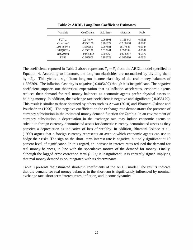
The results of the estimated long-run and short-run money demand function using three lags are
presented in Tables 2 and 3 below.
25
Table 2: ARDL Long-Run Coefficient Estimates Variable Coefficient Std. Error t-Statistic Prob.
-0.174874 0.064801 -1.155443 0.0525
-13.50136 0.766827 -17.60680 0.0000
( ) 1.586269 0.087881 26.77846 0.0044
( ) -0.053179 0.010241 2.097354 0.0382
- 0.005402 0.003265 -0.668207 0.5077
-0.885609 0.186722 -1.915680 0.0624
The coefficients reported in Table 2 above represents from the ARDL model specified in
Equation 4. According to literature, the long-run elasticities are normalised by dividing them
by . This yields a significant long-run income elasticity of the real money balances of
1.586269. The inflation elasticity is negative (-0.005402) though it is insignificant. The negative
coefficient supports our theoretical expectation that as inflation accelerates, economic agents
reduces their demand for real money balances as economic agents prefer physical assets to
holding money. In addition, the exchange rate coefficient is negative and significant (-0.053179).
This result is similar to those obtained by others such as Anwar (2010) and Bhamani-Oskoee and
Pourhedrian (1990). The negative coefficient on the exchange rate demonstrates the presence of
currency substitution in the estimated money demand function for Zambia. In an environment of
currency substitution, a depreciation in the exchange rate may induce economic agents to
substitute foreign currency-denominated assets for domestic currency-denominated assets as they
perceive a depreciation as indicative of loss of wealthy. In addition, Bhamani-Oskoee et al.,
(1990) argues that a foreign currency represents an avenue which economic agents can use to
hedge their risks. The sign on the short- term interest rate is negative, but only significant at 10
percent level of significance. In this regard, an increase in interest rates reduced the demand for
real money balances, in line with the speculative motive of the demand for money. Finally,
although the lagged error correction term (ECT) is insignificant, it is correctly signed implying
that real money demand is co-integrated with its determinants.
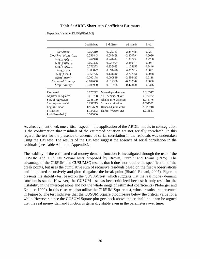
Table 3 presents the estimated short-run coefficients of the ARDL model. The results indicate
that the demand for real money balances in the short-run is significantly influenced by nominal
exchange rate, short-term interest rates, inflation, and income dynamics.
26
Table 3: ARDL Short-run Coefficient Estimates
Dependent Variable: DLOG(REALM2)
Coefficient Std. Error t-Statistic Prob.
0.054310 0.022747 2.387583 0.0201
( ) -0.256843 0.089468 -2.870794 0.0056
( ) 0.264940 0.241412 1.097459 0.2768
( ) 0.650475 0.228999 2.840518 0.0061
( ) 0.276273 0.235095 1.175157 0.2446
( ) 0.383827 0.094476 4.062712 0.0001
( ) -0.355775 0.131410 -2.707361 0.0088
( ) -0.002178 0.000839 -2.596422 0.0118
-0.107650 0.017356 -6.202544 0.0000
-0.008990 0.018988 -0.473434 0.6376
R-squared 0.675272 Mean dependent var 0.016517
Adjusted R-squared 0.615738 S.D. dependent var 0.077722
S.E. of regression 0.048179 Akaike info criterion -3.076776
Sum squared resid 0.139273 Schwarz criterion -2.697332
Log likelihood 122.7639 Hannan-Quinn criter. -2.925718
F-statistic 11.34273 Durbin-Watson stat 2.016581
Prob(F-statistic) 0.000000
As already mentioned, one critical aspect in the application of the ARDL models to cointegration
is the confirmation that residuals of the estimated equation are not serially correlated. In this
regard, the test for the presence or absence of serial correlation in the residuals was undertaken
using the LM test. The results of the LM test suggest the absence of serial correlation in the
residuals (see Table A4 in the Appendix).
The stability of the estimated real money demand function is investigated through the use of the
CUSUM and CUSUM Square tests proposed by Brown, Durbin and Evans (1975). The
advantage of the CUSUM and CUSUMSQ tests is that it does not require the specification of the
break points, but uses the cumulative sum of recursive residuals based on the first n observations
and is updated recursively and plotted against the break point (Sharifi-Renani, 2007). Figure 4
presents the stability test based on the CUSUM test, which suggests that the real money demand
function is stable. However, the CUSUM test has been criticized because it only tests for the
instability in the intercept alone and not the whole range of estimated coefficients (Ploberger and
Kramer, 1990). In this case, we also utilise the CUSUM Square test, whose results are presented
in Figure 5. The test indicates that the CUSUM Square plot crosses below the critical value for a
while. However, since the CUSUM Square plot gets back above the critical line it can be argued
that the real money demand function is generally stable even in the parameters over time.
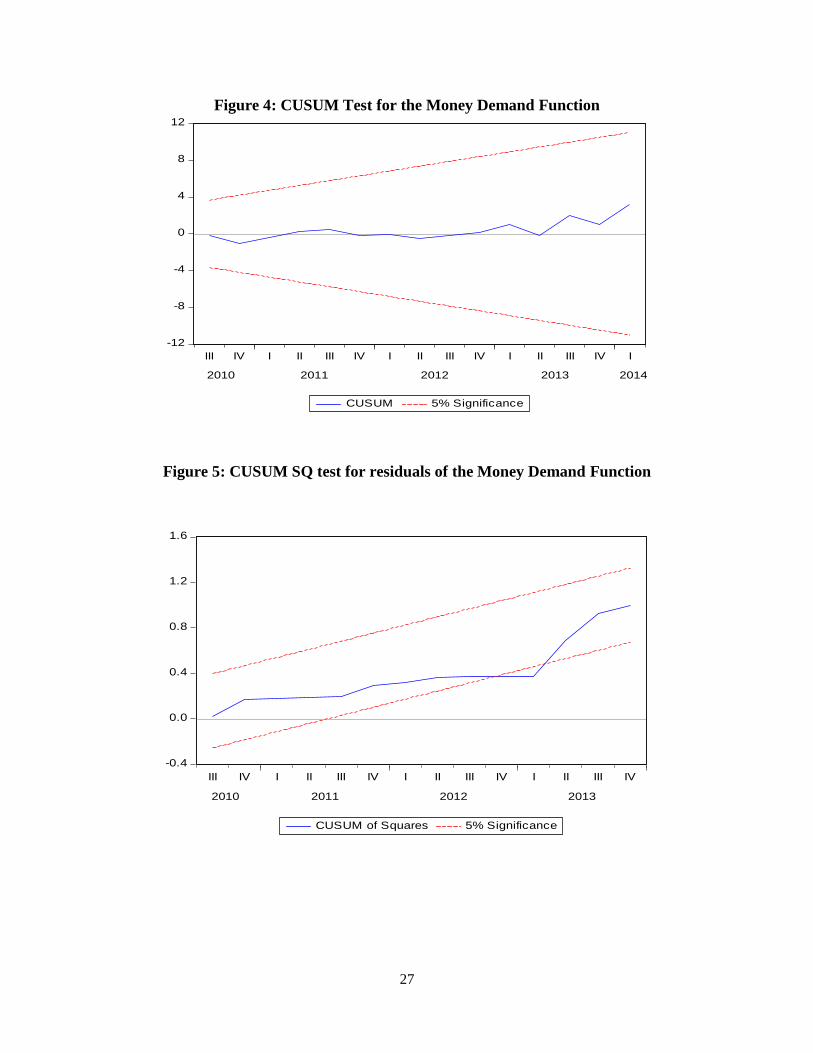
27
Figure 4: CUSUM Test for the Money Demand Function
-12
-8
-4
0
4
8
12
III IV I II III IV I II III IV I II III IV I
2010 2011 2012 2013 2014
CUSUM 5% Significance
Figure 5: CUSUM SQ test for residuals of the Money Demand Function
-0.4
0.0
0.4
0.8
1.2
1.6
III IV I II III IV I II III IV I II III IV
2010 2011 2012 2013
CUSUM of Squares 5% Significance
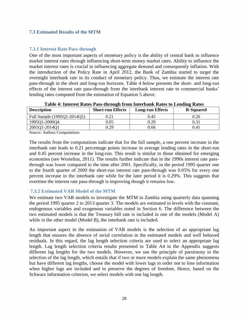
28
7.3 Estimated Results of the MTM
7.3.1 Interest Rate Pass-through
One of the most important aspects of monetary policy is the ability of central bank to influence
market interest rates through influencing short-term money market rates. Ability to influence the
market interest rates is crucial in influencing aggregate demand and consequently inflation. With
the introduction of the Policy Rate in April 2012, the Bank of Zambia started to target the
overnight interbank rate in its conduct of monetary policy. Thus, we estimate the interest rate
pass-through in the short and long-run horizons. Table 4 below presents the short- and long-run
effects of the interest rate pass-through from the interbank interest rate to commercial banks‘
lending rates computed from the estimation of Equation 5 above.
Table 4: Interest Rates Pass-through from Interbank Rates to Lending Rates
Description Short-run Effects Long-run Effects R-Squared
Full Sample (1995Q1-2014Q1) 0.21 0.45 0.26
1995Q1-2000Q4 0.05 0.29 0.31
2001Q1-2014Q1 0.29 0.66 0.41 Source: Authors Computations
The results from the computations indicate that for the full sample, a one percent increase in the
interbank rate leads to 0.21 percentage points increase in average lending rates in the short-run
and 0.45 percent increase in the long-run. This result is similar to those obtained for emerging
economies (see Westelius, 2011). The results further indicate that in the 1990s interest rate pass-
through was lower compared to the time after 2001. Specifically, in the period 1995 quarter one
to the fourth quarter of 2000 the short-run interest rate pass-through was 0.05% for every one
percent increase in the interbank rate while for the later period it is 0.29%. This suggests that
overtime the interest rate pass-through is improving though it remains low.
7.3.2 Estimated VAR Model of the MTM
We estimate two VAR models to investigate the MTM in Zambia using quarterly data spanning
the period 1995 quarter 2 to 2013 quarter 3. The models are estimated in levels with the constant,
endogenous variables and exogenous variables noted in Section 6. The difference between the
two estimated models is that the Treasury bill rate is included in one of the models (Model A)
while in the other model (Model B), the interbank rate is included.
An important aspect in the estimation of VAR models is the selection of an appropriate lag
length that ensures the absence of serial correlation in the estimated models and well behaved
residuals. In this regard, the lag length selection criteria are used to select an appropriate lag
length. Lag length selection criteria results presented in Table A4 in the Appendix suggests
different lag lengths for the two models. However, we use the principle of parsimony in the
selection of the lag length, which entails that if two or more models explain the same phenomena
but have different lag lengths, choose the model with lower lags in order not to lose information
when higher lags are included and to preserve the degrees of freedom. Hence, based on the
Schwarz information criterion, we select models with one lag length.
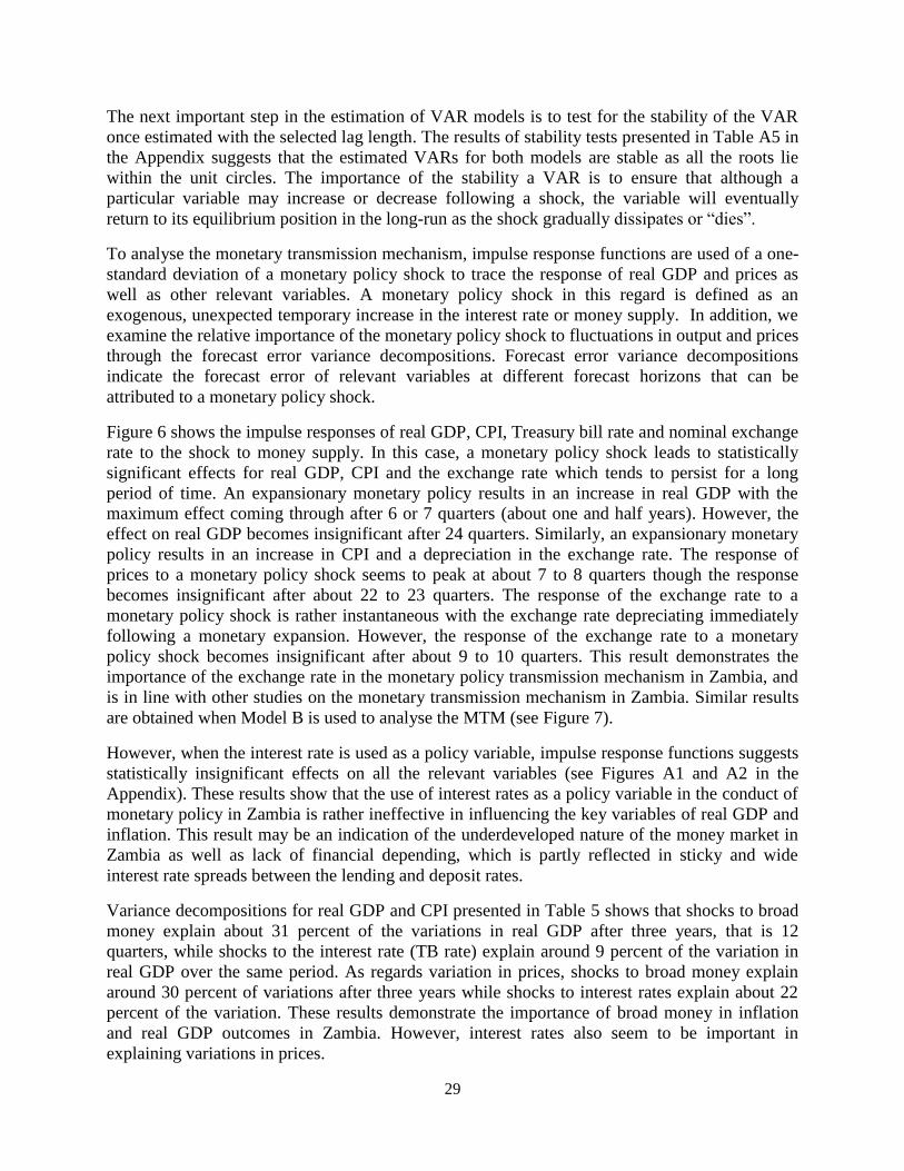
29
The next important step in the estimation of VAR models is to test for the stability of the VAR
once estimated with the selected lag length. The results of stability tests presented in Table A5 in
the Appendix suggests that the estimated VARs for both models are stable as all the roots lie
within the unit circles. The importance of the stability a VAR is to ensure that although a
particular variable may increase or decrease following a shock, the variable will eventually
return to its equilibrium position in the long-run as the shock gradually dissipates or ―dies‖.
To analyse the monetary transmission mechanism, impulse response functions are used of a one-
standard deviation of a monetary policy shock to trace the response of real GDP and prices as
well as other relevant variables. A monetary policy shock in this regard is defined as an
exogenous, unexpected temporary increase in the interest rate or money supply. In addition, we
examine the relative importance of the monetary policy shock to fluctuations in output and prices
through the forecast error variance decompositions. Forecast error variance decompositions
indicate the forecast error of relevant variables at different forecast horizons that can be
attributed to a monetary policy shock.
Figure 6 shows the impulse responses of real GDP, CPI, Treasury bill rate and nominal exchange
rate to the shock to money supply. In this case, a monetary policy shock leads to statistically
significant effects for real GDP, CPI and the exchange rate which tends to persist for a long
period of time. An expansionary monetary policy results in an increase in real GDP with the
maximum effect coming through after 6 or 7 quarters (about one and half years). However, the
effect on real GDP becomes insignificant after 24 quarters. Similarly, an expansionary monetary
policy results in an increase in CPI and a depreciation in the exchange rate. The response of
prices to a monetary policy shock seems to peak at about 7 to 8 quarters though the response
becomes insignificant after about 22 to 23 quarters. The response of the exchange rate to a
monetary policy shock is rather instantaneous with the exchange rate depreciating immediately
following a monetary expansion. However, the response of the exchange rate to a monetary
policy shock becomes insignificant after about 9 to 10 quarters. This result demonstrates the
importance of the exchange rate in the monetary policy transmission mechanism in Zambia, and
is in line with other studies on the monetary transmission mechanism in Zambia. Similar results
are obtained when Model B is used to analyse the MTM (see Figure 7).
However, when the interest rate is used as a policy variable, impulse response functions suggests
statistically insignificant effects on all the relevant variables (see Figures A1 and A2 in the
Appendix). These results show that the use of interest rates as a policy variable in the conduct of
monetary policy in Zambia is rather ineffective in influencing the key variables of real GDP and
inflation. This result may be an indication of the underdeveloped nature of the money market in
Zambia as well as lack of financial depending, which is partly reflected in sticky and wide
interest rate spreads between the lending and deposit rates.
Variance decompositions for real GDP and CPI presented in Table 5 shows that shocks to broad
money explain about 31 percent of the variations in real GDP after three years, that is 12
quarters, while shocks to the interest rate (TB rate) explain around 9 percent of the variation in
real GDP over the same period. As regards variation in prices, shocks to broad money explain
around 30 percent of variations after three years while shocks to interest rates explain about 22
percent of the variation. These results demonstrate the importance of broad money in inflation
and real GDP outcomes in Zambia. However, interest rates also seem to be important in
explaining variations in prices.
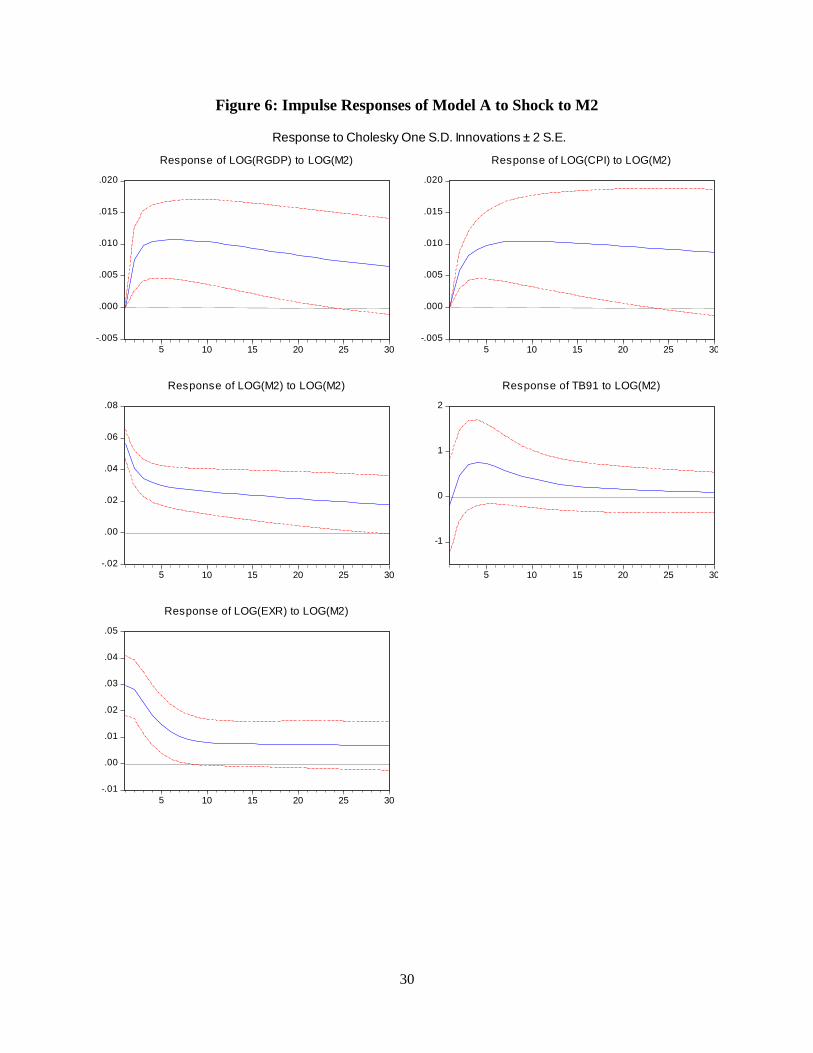
30
Figure 6: Impulse Responses of Model A to Shock to M2
-.005
.000
.005
.010
.015
.020
5 10 15 20 25 30
Response of LOG(RGDP) to LOG(M2)
-.005
.000
.005
.010
.015
.020
5 10 15 20 25 30
Response of LOG(CPI) to LOG(M2)
-.02
.00
.02
.04
.06
.08
5 10 15 20 25 30
Response of LOG(M2) to LOG(M2)
-1
0
1
2
5 10 15 20 25 30
Response of TB91 to LOG(M2)
-.01
.00
.01
.02
.03
.04
.05
5 10 15 20 25 30
Response of LOG(EXR) to LOG(M2)
Response to Cholesky One S.D. Innovations ± 2 S.E.
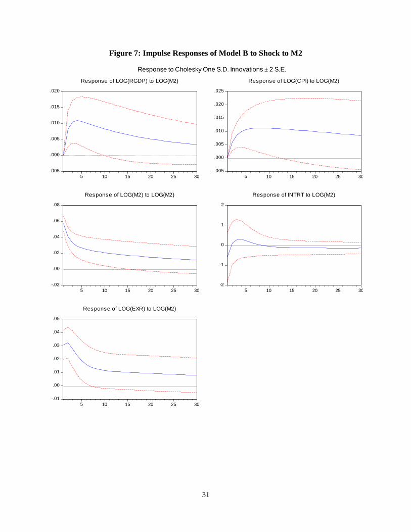
31
Figure 7: Impulse Responses of Model B to Shock to M2
-.005
.000
.005
.010
.015
.020
5 10 15 20 25 30
Response of LOG(RGDP) to LOG(M2)
-.005
.000
.005
.010
.015
.020
.025
5 10 15 20 25 30
Response of LOG(CPI) to LOG(M2)
-.02
.00
.02
.04
.06
.08
5 10 15 20 25 30
Response of LOG(M2) to LOG(M2)
-2
-1
0
1
2
5 10 15 20 25 30
Response of INTRT to LOG(M2)
-.01
.00
.01
.02
.03
.04
.05
5 10 15 20 25 30
Response of LOG(EXR) to LOG(M2)
Response to Cholesky One S.D. Innovations ± 2 S.E.
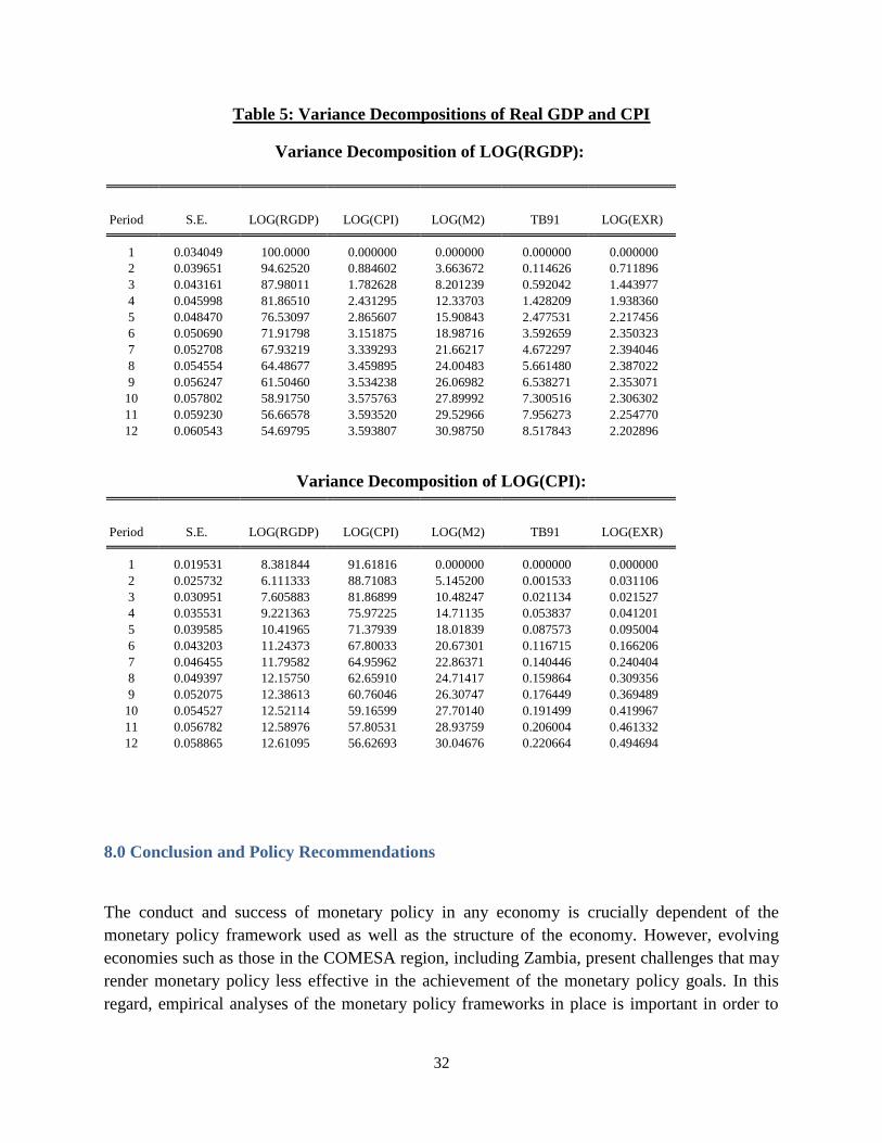
32
Table 5: Variance Decompositions of Real GDP and CPI
Variance Decomposition of LOG(RGDP):
Period S.E. LOG(RGDP) LOG(CPI) LOG(M2) TB91 LOG(EXR)
1 0.034049 100.0000 0.000000 0.000000 0.000000 0.000000
2 0.039651 94.62520 0.884602 3.663672 0.114626 0.711896
3 0.043161 87.98011 1.782628 8.201239 0.592042 1.443977
4 0.045998 81.86510 2.431295 12.33703 1.428209 1.938360
5 0.048470 76.53097 2.865607 15.90843 2.477531 2.217456
6 0.050690 71.91798 3.151875 18.98716 3.592659 2.350323
7 0.052708 67.93219 3.339293 21.66217 4.672297 2.394046
8 0.054554 64.48677 3.459895 24.00483 5.661480 2.387022
9 0.056247 61.50460 3.534238 26.06982 6.538271 2.353071
10 0.057802 58.91750 3.575763 27.89992 7.300516 2.306302
11 0.059230 56.66578 3.593520 29.52966 7.956273 2.254770
12 0.060543 54.69795 3.593807 30.98750 8.517843 2.202896
Variance Decomposition of LOG(CPI):
Period S.E. LOG(RGDP) LOG(CPI) LOG(M2) TB91 LOG(EXR)
1 0.019531 8.381844 91.61816 0.000000 0.000000 0.000000
2 0.025732 6.111333 88.71083 5.145200 0.001533 0.031106
3 0.030951 7.605883 81.86899 10.48247 0.021134 0.021527
4 0.035531 9.221363 75.97225 14.71135 0.053837 0.041201
5 0.039585 10.41965 71.37939 18.01839 0.087573 0.095004
6 0.043203 11.24373 67.80033 20.67301 0.116715 0.166206
7 0.046455 11.79582 64.95962 22.86371 0.140446 0.240404
8 0.049397 12.15750 62.65910 24.71417 0.159864 0.309356
9 0.052075 12.38613 60.76046 26.30747 0.176449 0.369489
10 0.054527 12.52114 59.16599 27.70140 0.191499 0.419967
11 0.056782 12.58976 57.80531 28.93759 0.206004 0.461332
12 0.058865 12.61095 56.62693 30.04676 0.220664 0.494694
8.0 Conclusion and Policy Recommendations
The conduct and success of monetary policy in any economy is crucially dependent of the
monetary policy framework used as well as the structure of the economy. However, evolving
economies such as those in the COMESA region, including Zambia, present challenges that may
render monetary policy less effective in the achievement of the monetary policy goals. In this
regard, empirical analyses of the monetary policy frameworks in place is important in order to
33
assess the effectiveness of the frameworks and to design frameworks that will yield the desired
goals, if existing frameworks are found to be ineffective.
The empirical analyses undertaken in this study regarding the money demand function in Zambia
suggest a generally stable money demand function. This result implies that monetary aggregates
can still play a critical role in monetary policy implementation in Zambia, and possibly in other
COMESA member countries that have been using a similar framework. The results from the
VAR analysis of the monetary transmission mechanism also support the importance of monetary
aggregates in the conduct of monetary policy given the significant effects that monetary
aggregates have on output and prices.
However, the weakening link between consumer prices and monetary aggregates would naturally
require that the Bank of Zambia—along with many other central banks in similar situations—
starts the search for a policy framework that will be more effective in the future conduct of
monetary policy, such as inflation targeting which focuses on targeting inflation through a policy
rate instead of focusing on maintaining a certain growth rate in money aggregates.
The overall recommendation from this study is that as the process of modernising monetary
policy frameworks gets underway to address the emerging economic challenges, it is clear that in
the case of Zambia monetary aggregates will still continue to play a role in monetary policy
conduct. In this regard, it would be premature to abandon the traditional policy focus on
monetary aggregates, given their influence on the key macroeconomic outcomes of output and
prices. A key implication from this study is therefore that monetary policy in Zambia, and other
COMESA member countries, should continue to consider developments in monetary aggregates
while gradually transitioning to modern monetary policy frameworks. In addition, measures
should be put in place that are aimed at enhancing monetary transmission mechanisms,
particularly the interest rate channel, by promoting financial deepening and economic
development more generally.
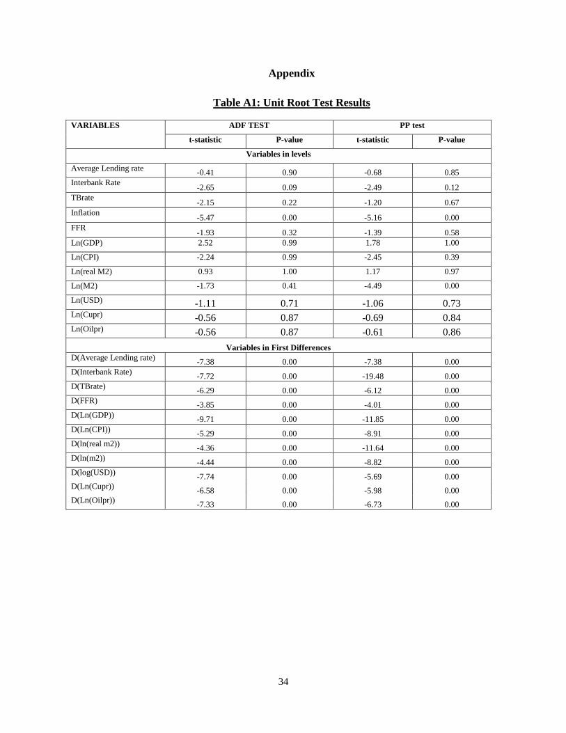
34
Appendix
Table A1: Unit Root Test Results
VARIABLES ADF TEST PP test
t-statistic P-value t-statistic P-value
Variables in levels
Average Lending rate -0.41 0.90 -0.68 0.85
Interbank Rate -2.65 0.09 -2.49 0.12
TBrate -2.15 0.22 -1.20 0.67
Inflation -5.47 0.00 -5.16 0.00
FFR -1.93 0.32 -1.39 0.58
Ln(GDP) 2.52 0.99 1.78 1.00
Ln(CPI) -2.24 0.99 -2.45 0.39
Ln(real M2) 0.93 1.00 1.17 0.97
Ln(M2) -1.73 0.41 -4.49 0.00
Ln(USD) -1.11 0.71 -1.06 0.73 Ln(Cupr) -0.56 0.87 -0.69 0.84 Ln(Oilpr) -0.56 0.87 -0.61 0.86
Variables in First Differences
D(Average Lending rate) -7.38 0.00 -7.38 0.00
D(Interbank Rate) -7.72 0.00 -19.48 0.00
D(TBrate) -6.29 0.00 -6.12 0.00
D(FFR) -3.85 0.00 -4.01 0.00
D(Ln(GDP)) -9.71 0.00 -11.85 0.00
D(Ln(CPI)) -5.29 0.00 -8.91 0.00
D(ln(real m2)) -4.36 0.00 -11.64 0.00
D(ln(m2)) -4.44 0.00 -8.82 0.00
D(log(USD)) -7.74 0.00 -5.69 0.00
D(Ln(Cupr)) -6.58 0.00 -5.98 0.00
D(Ln(Oilpr)) -7.33 0.00 -6.73 0.00
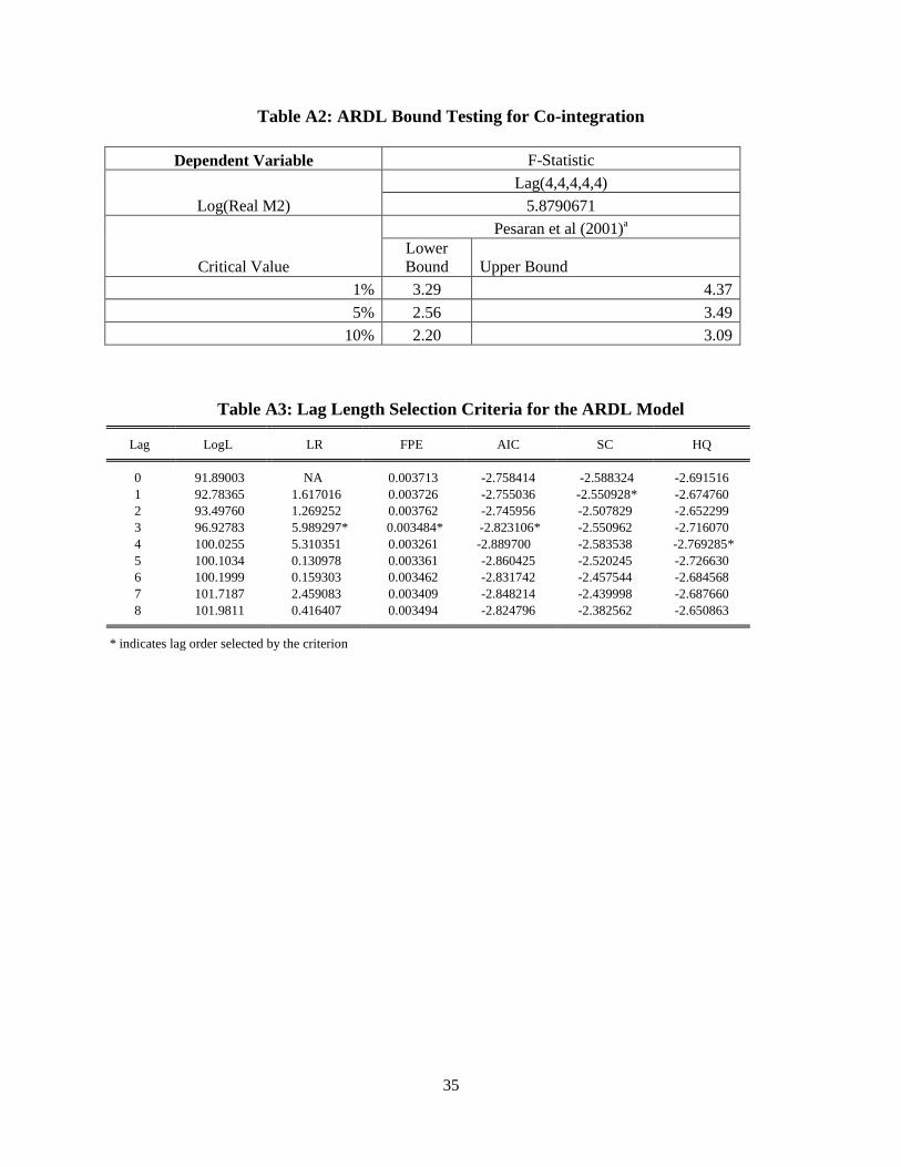
35
Table A2: ARDL Bound Testing for Co-integration
Dependent Variable F-Statistic
Log(Real M2)
Lag(4,4,4,4,4)
5.8790671
Critical Value
Pesaran et al (2001)a
Lower
Bound Upper Bound
1% 3.29 4.37
5% 2.56 3.49
10% 2.20 3.09
Table A3: Lag Length Selection Criteria for the ARDL Model Lag LogL LR FPE AIC SC HQ
0 91.89003 NA 0.003713 -2.758414 -2.588324 -2.691516
1 92.78365 1.617016 0.003726 -2.755036 -2.550928* -2.674760
2 93.49760 1.269252 0.003762 -2.745956 -2.507829 -2.652299
3 96.92783 5.989297* 0.003484* -2.823106* -2.550962 -2.716070
4 100.0255 5.310351 0.003261 -2.889700 -2.583538 -2.769285*
5 100.1034 0.130978 0.003361 -2.860425 -2.520245 -2.726630
6 100.1999 0.159303 0.003462 -2.831742 -2.457544 -2.684568
7 101.7187 2.459083 0.003409 -2.848214 -2.439998 -2.687660
8 101.9811 0.416407 0.003494 -2.824796 -2.382562 -2.650863
* indicates lag order selected by the criterion
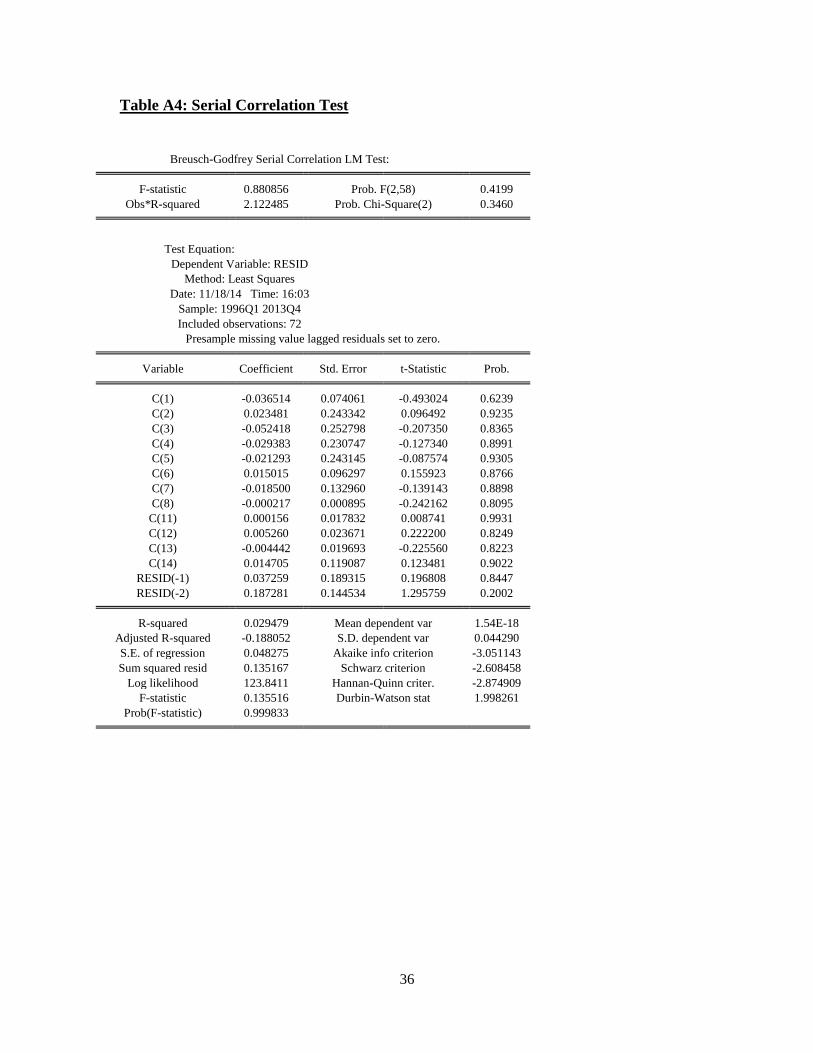
36
Table A4: Serial Correlation Test
Breusch-Godfrey Serial Correlation LM Test:
F-statistic 0.880856 Prob. F(2,58) 0.4199
Obs*R-squared 2.122485 Prob. Chi-Square(2) 0.3460
Test Equation:
Dependent Variable: RESID
Method: Least Squares
Date: 11/18/14 Time: 16:03
Sample: 1996Q1 2013Q4
Included observations: 72
Presample missing value lagged residuals set to zero.
Variable Coefficient Std. Error t-Statistic Prob.
C(1) -0.036514 0.074061 -0.493024 0.6239
C(2) 0.023481 0.243342 0.096492 0.9235
C(3) -0.052418 0.252798 -0.207350 0.8365
C(4) -0.029383 0.230747 -0.127340 0.8991
C(5) -0.021293 0.243145 -0.087574 0.9305
C(6) 0.015015 0.096297 0.155923 0.8766
C(7) -0.018500 0.132960 -0.139143 0.8898
C(8) -0.000217 0.000895 -0.242162 0.8095
C(11) 0.000156 0.017832 0.008741 0.9931
C(12) 0.005260 0.023671 0.222200 0.8249
C(13) -0.004442 0.019693 -0.225560 0.8223
C(14) 0.014705 0.119087 0.123481 0.9022
RESID(-1) 0.037259 0.189315 0.196808 0.8447
RESID(-2) 0.187281 0.144534 1.295759 0.2002
R-squared 0.029479 Mean dependent var 1.54E-18
Adjusted R-squared -0.188052 S.D. dependent var 0.044290
S.E. of regression 0.048275 Akaike info criterion -3.051143
Sum squared resid 0.135167 Schwarz criterion -2.608458
Log likelihood 123.8411 Hannan-Quinn criter. -2.874909
F-statistic 0.135516 Durbin-Watson stat 1.998261
Prob(F-statistic) 0.999833
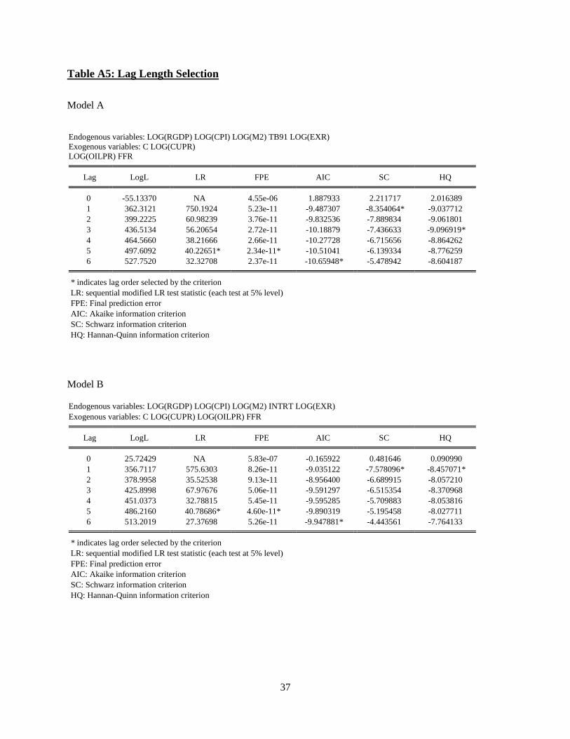
37
Table A5: Lag Length Selection
Model A
Endogenous variables: LOG(RGDP) LOG(CPI) LOG(M2) TB91 LOG(EXR)
Exogenous variables: C LOG(CUPR)
LOG(OILPR) FFR
Lag LogL LR FPE AIC SC HQ
0 -55.13370 NA 4.55e-06 1.887933 2.211717 2.016389
1 362.3121 750.1924 5.23e-11 -9.487307 -8.354064* -9.037712
2 399.2225 60.98239 3.76e-11 -9.832536 -7.889834 -9.061801
3 436.5134 56.20654 2.72e-11 -10.18879 -7.436633 -9.096919*
4 464.5660 38.21666 2.66e-11 -10.27728 -6.715656 -8.864262
5 497.6092 40.22651* 2.34e-11* -10.51041 -6.139334 -8.776259
6 527.7520 32.32708 2.37e-11 -10.65948* -5.478942 -8.604187
* indicates lag order selected by the criterion
LR: sequential modified LR test statistic (each test at 5% level)
FPE: Final prediction error
AIC: Akaike information criterion
SC: Schwarz information criterion
HQ: Hannan-Quinn information criterion
Model B
Endogenous variables: LOG(RGDP) LOG(CPI) LOG(M2) INTRT LOG(EXR)
Exogenous variables: C LOG(CUPR) LOG(OILPR) FFR
Lag LogL LR FPE AIC SC HQ
0 25.72429 NA 5.83e-07 -0.165922 0.481646 0.090990
1 356.7117 575.6303 8.26e-11 -9.035122 -7.578096* -8.457071*
2 378.9958 35.52538 9.13e-11 -8.956400 -6.689915 -8.057210
3 425.8998 67.97676 5.06e-11 -9.591297 -6.515354 -8.370968
4 451.0373 32.78815 5.45e-11 -9.595285 -5.709883 -8.053816
5 486.2160 40.78686* 4.60e-11* -9.890319 -5.195458 -8.027711
6 513.2019 27.37698 5.26e-11 -9.947881* -4.443561 -7.764133
* indicates lag order selected by the criterion
LR: sequential modified LR test statistic (each test at 5% level)
FPE: Final prediction error
AIC: Akaike information criterion
SC: Schwarz information criterion
HQ: Hannan-Quinn information criterion
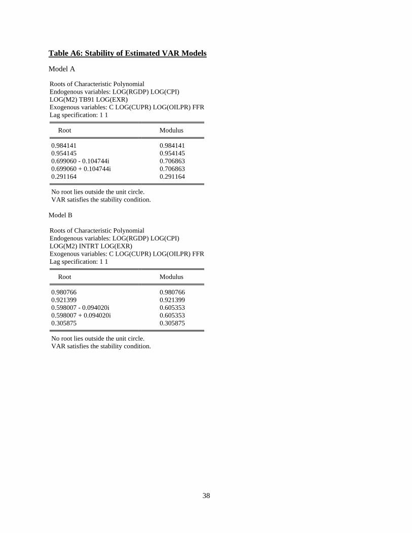
38
Table A6: Stability of Estimated VAR Models
Model A
Roots of Characteristic Polynomial
Endogenous variables: LOG(RGDP) LOG(CPI)
LOG(M2) TB91 LOG(EXR)
Exogenous variables: C LOG(CUPR) LOG(OILPR) FFR
Lag specification: 1 1
Root Modulus
0.984141 0.984141
0.954145 0.954145
0.699060 - 0.104744i 0.706863
0.699060 + 0.104744i 0.706863
0.291164 0.291164
No root lies outside the unit circle.
VAR satisfies the stability condition.
Model B
Roots of Characteristic Polynomial
Endogenous variables: LOG(RGDP) LOG(CPI)
LOG(M2) INTRT LOG(EXR)
Exogenous variables: C LOG(CUPR) LOG(OILPR) FFR
Lag specification: 1 1
Root Modulus
0.980766 0.980766
0.921399 0.921399
0.598007 - 0.094020i 0.605353
0.598007 + 0.094020i 0.605353
0.305875 0.305875
No root lies outside the unit circle.
VAR satisfies the stability condition.
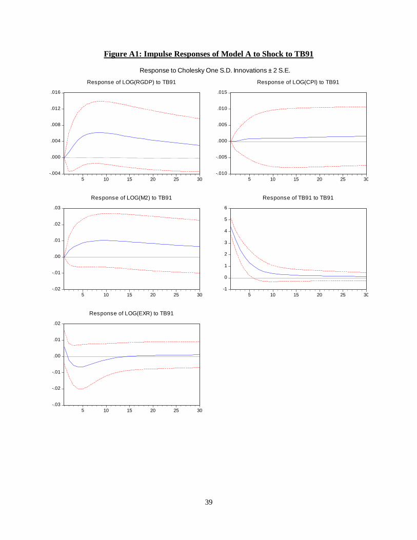
39
Figure A1: Impulse Responses of Model A to Shock to TB91
-.004
.000
.004
.008
.012
.016
5 10 15 20 25 30
Response of LOG(RGDP) to TB91
-.010
-.005
.000
.005
.010
.015
5 10 15 20 25 30
Response of LOG(CPI) to TB91
-.02
-.01
.00
.01
.02
.03
5 10 15 20 25 30
Response of LOG(M2) to TB91
-1
0
1
2
3
4
5
6
5 10 15 20 25 30
Response of TB91 to TB91
-.03
-.02
-.01
.00
.01
.02
5 10 15 20 25 30
Response of LOG(EXR) to TB91
Response to Cholesky One S.D. Innovations ± 2 S.E.
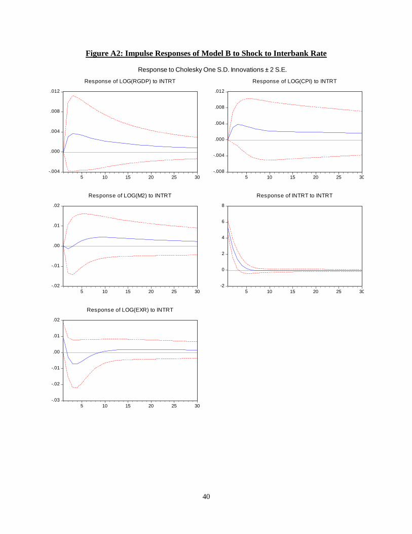
40
Figure A2: Impulse Responses of Model B to Shock to Interbank Rate
-.004
.000
.004
.008
.012
5 10 15 20 25 30
Response of LOG(RGDP) to INTRT
-.008
-.004
.000
.004
.008
.012
5 10 15 20 25 30
Response of LOG(CPI) to INTRT
-.02
-.01
.00
.01
.02
5 10 15 20 25 30
Response of LOG(M2) to INTRT
-2
0
2
4
6
8
5 10 15 20 25 30
Response of INTRT to INTRT
-.03
-.02
-.01
.00
.01
.02
5 10 15 20 25 30
Response of LOG(EXR) to INTRT
Response to Cholesky One S.D. Innovations ± 2 S.E.
41
References
Adam, C.S., 1999. ―Financial Liberalisation and Currency Demand in Zambia‖, Journal of
African Economies, Vol. 8 (3)
Afandi, A., 2005. ―Monetary Policy Transmission Mechanism and Structural breaks in
Indonesia‖, PhD Thesis, School of Economics and Information Systems, University of
Wollongong.
Anwar, S. and N. Asghar. 2012. ―Is the Demand for money Stable in Pakistan?‖ Pakistan
Economic and Social Review Vol. 50(1): 1-22.
Ando, Albert, and Franco Modigliani. 1963. ―The ‗life-cycle‘ hypothesis of saving: aggregate
implications and tests‖, American Economic Review, 53(1), 55–84.
Alper, K. 2003. ―Exchange Rate Pass-through to Domestic Prices in Turkish Economy‖, MSc
Thesis, Middle East Technical University
Bahmani-Oskooee, M. and Mohammad Pourhedarian. 1990. ―Exchange rate sensitivity of
demand for money and effectiveness of fiscal and monetary policies‖, Applied Economics,
Volume 22, No. 7, pp. 917-925.
Bahmani, S. and M. Bahmani-Oskoee. 1996. ―Exchange Rate Volatility and Demand for Money
in Iran‖ Available online at:
http://iraneconomy.csames.illinois.edu/full%20papers/Bahmani%20-
%20Exchange%20Rate%20Volatility%20and%20Demand%20for%20Money%20in%20Iran.pdf
Bank of England, 1999. ―The Transmission Mechanism of Monetary Policy,‖ Bank of England
Quarterly Bulletin, May, pp. 161-70
Baumal, W.J., 1952. ―The Transactions demand for Cash: An Inventory Theoretic Approach,‖
Quarterly Journal of Economics 66. pp. 545-556.
Bernanke B. and A. Blinder. 1992. ―The Federal Funds Rate and the Channels of
42
Monetary Transmission,‖ American Economic Review Vol. 82: 901-21.
Bernanke, B.S. and M. Gertler. 1995. ―Inside the black box: the credit channel of monetary
policy transmission,‖ .Journal of Economic Perspectives, Vol. 9(4), 27-48.
Bernanke, B. 2006. ―Monetary Aggregates and Monetary Policy at the Federal Reserve: A
Historical Perspective,‖ Paper presented at the fourth ECB Central Banking Conference.
Bigstern, A. and Mugerwa-Kiyizzi, S. 2000. ―The Political Economy of Policy Failure in
Zambia‖, Working Paper in Economics No. 23/00, University of Gothenburg.
Blanchard, O. 2000. ―What do we know about Macroeconomics that Fisher and Wicksell did
not?‖ NBER Working Paper 7550.
Boivin J. M., M. Kiley and F. Mishkin. 2010. ―How has the Monetary Transmission Mechanism
Evolved over Time?‖ NBER Working Paper, No. 15879.
Bordon, A.R. and A Weber. 2010. ―The transmission mechanism in Armenia: new evidence
from a regime switching VAR analysis,‖ IMF Working Paper No. 270.
Bova, E., 2009. ―Is the Zambian Kwacha a Commodity Currency? The Co-movement between
Copper Prices and the Exchange Rate,‖ Swiss National Centre for Competence in Research
Working Paper No. 2009/11
Brown, R.L., J. Durbin and J.M. Evans (1975).―Techniques for Testing the Constancy of
Regression Relationships over Time,‖ Journal of the Royal Statistical Society, Series B, 35, 149-
192.
Butkiewcz J. and ZelilaOzdogan. 2008. ―Financial crisis, monetary policy reform and the
monetary transmission mechanism in Turkey‖. Turkey: SBT analysis
43
Campa, J. and L. Goldberg.2004. ―Exchange Rate Pass-through into Import Prices: A Macro or
Micro Phenomenon?‖ NBER Working Paper 8934.
Carter, T. J. 2005. ―Monetary Policy, Efficiency Wages, and Nominal Rigidities,‖ .Eastern
Economic Journal, vol. 31, No. 3; 349-359.
Cevik S. And K. Teksoz. 2012. ―Lost in Transmission? The Effectiveness of Monetary Policy
Transmission Channels in the GCC countries,‖ IMF Working Paper no. 12/191.
Cheng, K.C., 2006. ―A VAR Analysis of Kenya‘s Monetary Transmission Mechanism: How
Does the Central Bank‘s Repo Rate Affect the Economy?‖, IMF Working Paper No. 06/300
Christiano, L. J., M. Eichenbaum. 1992. ―Identification and the Liquidity Effect of a Monetary
Policy Shock‖, in Political Economy, Growth and Business Cycles, A. Cukierman, Z. Hercowitz
and L. Liederman, (eds), Cambridge and London; MIT Press.
Dabla-Norris E. and Holger Floerkemeier. 2006. ―Transmission Mechanisms of Monetary Policy
in Armenia: Evidence from VAR Analysis,‖ IMF Working Paper, No. 06/248.
Dagher, J. and A. Kovanen, 2011. ―On the Stability of Money Demand in Ghana: A Bounds
Testing Approach,‖ IMF Working Paper No. 11/273
Davoodi, H., S. Dixit, and G. Pinter, 2013. ―Monetary Transmission Mechanisms in the East
African Community: An Empirical Investigation,‖ IMF Working Paper No. 39/2013
Dornbusch, R., 1976. ―Expectations and Exchange Rate Dynamics,‖ Journal of Political
Economy, Vol. 84, pp. 1161 - 1176
Espinoza, R. and Prasad, A., 2012. ―Monetary Policy Transmission in the GCC Countries,‖ IMF
Working Paper No. 2012/132
44
Fleming, J.M. 1962. ―Domestic Financial Polices Under Fixed and Under Floating Exchange
Rates,‖ IMF Staff Papers no. 9: 369–79.
Friedman, M., 1956. ―The Quantity Theory of Money – A Re-statement,‖ in M. Friedman, ed,
Studies in Quantity Theory of Money. University of Chicago Press, pp. 3 - 21
Friedman, M. 1968. The Role of Monetary Policy.American Economic Review, Vol. 58; 1-17.
Friedman M., and Anna Schwartz. 1971. A Monetary History of the United States, 1967-1960.
Princeton: NBER.
Friedman, B. and Kuttner, K. Money, Income, Prices and Interest Rates American Economic
Review 82. June, 1982.
Handa, Jagdish. 2009. Monetary Economics, Second Edition, Routledge.
Hannsgen, G. 2004. ―The Transmission Mechanism of Monetary Policy: A Critical Review,‖
The Levy Economics Institute Working Paper No. 412.
Horvath, B. and R. Maino, 2006. ―Monetary Transmission Mechanisms in Belurus,‖ IMF
Working Paper No.2006/246
Ireland, P. 2005. ―The Monetary Transmission Mechanism,‖ Federal Reserve Bank of Boston
Working Papers, No. 06/1.
Kakes, J. 2000. Monetary Transmission in Europe-The role of Financial Markets and Credit.
Edward Elgar Publishing.
Kalyalya, D.H (2001), ―Monetary Policy Framework and Implementation in Zambia‖, paper
presented at the SARB Conference on Monetary Policy Frameworks.
Kamin, S., P. Turner, and J. Van‘tdack.1998.‖The Transmission Mechanism of Monetary Policy
in Emerging Market Economies: An Overview,‖ BIS Policy Papers No. 3, 5-64.
45
Kara, Hakan, HandeKucukTuger, UmitOzlale, BurcTuger, DevrimYavuz, and ErayYucel. 2005.
―Exchange Rate Pass Through in Turkey: Has It Changed, and to What Extend?‖ Research
Department Working Papers, No: 05/04, The Central Bank of Republic of Turkey
Kassim S.H., M.S. A. Majid. 2008. ―The Role of Bank Lending in the Monetary Transmission
Process of a Developing Economy: Evidence from Malaysia,‖ Savings and Development, Vol.
32(4).
Keynes, J.M. 1936. The General Theory of Employment, Interest and Money. London;
Macmillan.
Keynes, J. M. 1937. ―The General Theory of Employment,‖ Quarterly Journal of Economics vol
51; 209-223.
King R. and C. Plosser. 1984. ―Money, Credit and Prices in a Real Business Cycle,‖ American
Economic Review, vol. 74; 363-80.
Kuttner, K., and P. Mosser.2000.‖The Monetary Transmission Mechanism: Some Answers and
Further Questions,‖ Federal Reserve Bank of New York Economic Policy Review.
Kydland, F. And E. Prescott. 1982. ―Time to Build and Aggregate Fluctuations,‖ Econometrica,
vol. 50; 1345-70.
Lucas R. E. ([1972] 1981). ―Expectations and the Neutrality of Money,‖ reprinted in Studies in
Business Cycle theory, Cambridge: MIT press; 65-89.
Loazya, N. and K. Schmidt-Hebbel. 2002. ―Monetary Policy Functions and Transmission
Mechanisms: An Overview,‖ In Loazya and Schmidt-Hebbel (eds), ―Monetary Policy: Rules and
Transmission Mechanisms, Santiago; Central Bank of Chile.
Long, J. and C. Plosser. 1983. ―Real Business Cycles,‖ Journal of Political Economy, vol. 94;
39-69.
46
Lungu, M., Simwaka, K., Chiumia, A., Palamuleni. A., and Jombo, W. 2012. ―Money Demand
Function for Malawi – Implications for Monetary Policy Conduct,‖ Banks and Bank Systems,
Volume 7, Issue 1.
Maturu, O.B., 2014, ―Short-term Capital Flows and Pressure on the Exchange Rate in Kenya,‖
Paper presented at the Centre for Studies of African Economies (CSAE) Annual Conference, 23
– 25th
March, 2014.
Mabrouk A. F., S. M. Hassan. 2012. ―Evolution of Monetary Policy in Egypt: A Critical
Review,‖ The International Journal of Social Sciences Vol. 4 no. 1
McCallum, B.T., and E. Nelson.2001. ―Monetary Policy for an Open Economy: An Alternative
Framework with Optimizing Agents and Sticky Prices,” NBER Working Paper No: 8175.
Meltzer, A. H. 1995. ―Monetary, Credit, and (Other) Transmission Processes: A Monetarist
Perspective,‖ Journal of Economic Perspectives, vol. 9 no. 4: 49-72.
Mishkin, S. F., 1995. ―Symposium on the Monetary Transmission Mechanisms,‖ Journal of
Economic Perspectives, Vol. 9, pp. 49 – 72.
Mishkin, S. F. 2007. The economics of Money, Banking and Financial Markets, ed. USA;
Pearson-Addison-Wesley.
Mishkin, S. F. 2001. ―The Inexorable and Mysterious Trade-off between Inflation and
Unemployment,‖ Economic Journal, vol. 111: C45-C61.
Mishkin S. F. 2001. ―The Transmission Mechanism and the Role of Asset prices in Monetary
Policy,‖ NBER Working Paper no.8617.
Mishkin, F. 1996. ―The Channels of Monetary Transmission: Lessons for Monetary Policy,‖
NBER Working Paper, No. 5464.
Mishra, P. and P. Montiel and A. Spilimbergo. 2010. ―Monetary Transmission in Low Income
Countries,‖ IMF Working Paper, No. 10/223.
47
Mundell, R.A. 1963.‖Capital Mobility and Stabilization Policy under Fixed and Flexible
Exchange Rates,‖ Canadian Journal of Economics and Political Science vol.29: 475–485.
Mutoti, N., 2006. ―Monetary Policy Transmission Mechanisms in Zambia,‖ Bank of Zambia
Working Papers (WP/06/2006).
Mutoti, N., Kapembwa, C., and Zgambo, P., 2010, ―Inflation Targeting in Zambia,‖ Unpublished
Bank of Zambia Working Paper.
Mwansa, L., 1998, ―Determinants of Inflation in Zambia,‖ PhD Dissertation, University of
Gothenburg, Sweden.
Mwenda, A, 1993, ― Credit rationing in Investment Behaviour under Market Imperfections‖.
Ph.D. Thesis, University of Gothenborg, Gothenborg
Obstfeld, M., and K. Rogoff, 1995. ―Exchange Rate Dynamics Redux,‖ Journal of Political
Economy, vol. 103: 624–660.
Ogunsakin, S. and A.A. Awe, 2014. ―Impact of Financial Liberalisation on the Stability of
Nigerian Money Demand Function,‖ International Journal of Economics, Business and Finance,
Vol. 2, No.1, pp. 1 – 18
Ozdogan Z. 2009. ―Monetary Transmission Mechanism in Turkey‖, PhD Dissertation:
University of Delaware
Pesaran, M. H., Yongcheol Shin and R. J. Smith .2001. ―Bounds testing approaches to the
analysis of level relationships,‖ Journal of Applied Econometrics, Volume 16(3): pp.289-326.
Phelps, E.And J. Taylor. 1977. ―Stabilizing Powers of Monetary Policy under Rational
Expectations,‖ Journal of Political Economy, vol. 85; 163-190.
Phillip, C. 1965. ―Determinants and Effects of Changes in Stock of Money,‖ NBER working
paper 13.
48
Ploberger, W. and W. Kramer (1990), "The Local Power of the CUSUM and
CUSUM of Squares Tests," Econometric Theory, 6, 335-347.
Poole, W. 1970.‖Optimal Choice of Monetary Policy Instruments in a Simple Stochastic Macro
Model,‖Quarterly Journal of Economics.
Putkuri, H. 2003.‖ Cross-country asymmetries in euro area monetary transmission: the role of
national financial systems,‖ Discussion Paper No. 15, Bank of Finland.
Roberts, J. 1987. ―An Equilibrium Model with Involuntary Unemployment at Flexible
Competitive Prices and Wages,‖ .American Economic Review, vol. 77; 856-74.
Rogoff, K. 1989. ―Reputation, Coordination, and Monetary Policy,‖ in R. Barro ed., Modern
Business Cycle Theory, Cambridge: Harvard University Press.
Romer, D. 2006. Advanced Macroeconomics, Third Edition, McGraw-Hill.
Rothbard, M. 2009. ―Economic Depressions: Their Cause and Cure,‖ Ludwig Von Mises
Institute, USA.
Salop, S. 1979. ―A Model of the Natural Rate of Unemployment.America,‖ Economic Review,
Vol. 74; 433-44.
Samuelson, P and Nordhaus, W. 2004.Economics; McGraw Hill.
Sawar, H. Sawar, M. and M. Waqas, 2013, ―Stability of Money Demand Function in Pakistan,‖
Economic and Political Review, Vol. 15, No. 3, pp. 197 - 212
49
Shapiro, C. and J.E Stiglitz. 1984. ―Equilibrium Unemployment as Per Worker Discipline,‖
American Economic Review, vol. 74: 177-94.
Sharifi-Renani, H. 2007, ―Demand for Money in Iran: An ARDL Approach,‖ Munich Personal
RePEc Archive (MPRA)
Simatele, M.C.H., 2004, ―Financial Sector Reforms and Monetary Policy Reforms in Zambia,‖
PhD Dissertation, University of Gothenburg, Sweden
Smith, A. 1776. AnInquiry into the Nature and Causes of the Wealth of Nations. London
Sriram S.S, 1999. ―The Demand for M2 in Malaysia‖, PhD dissertation: George Washington
University.
Stein, L. J. 1981. ―Monetarist, Keynesians and new Classical Economics,‖ American Economic
Review, vol. 71 issue 2: 139-44.
Tahir M. N. 2012. ―Relative Importance of Monetary Transmission Channels: A Structural
Investigation; A case of Brazil, Chile and Korea,‖ University of Lyon Working paper Series.
Tahir, M. N. 2009. ―Essays in Inflation and Monetary Policy Dynamics in a Globalised world‖,
Unpublished Dissertation: University of Leuven.
Taylor, J. B. 1979. ―Estimation and Control of an Econometric Model with Rational
Expectations,‖ Econometrica, vol. 47; 1267-86.
Taylor, J.B. 1993. ―Discretion versus Policy Rules in Practice,‖ Carnegie Rochester Conference
Series on Public Policy, vol. 39: 195–214.
Taylor, J.B.1995. ―The monetary transmission mechanism: an empirical framework.‖ .Journal of
Economic Perspectives, vol. 9(4), 11-26.
50
Taylor J.B. 1999. The Monetary transmission Mechanism and the Evaluation of Monetary Policy
Rules. Prepared for third annual international conference of the central bank of Chile on
―Monetary policy: Rules and Transmission mechanisms‖ September, 1999.
Tobin, J., 1956, ―The Interest elasticity of Transactions demand for Cash,‖ Review of Economics
and Statistics 38: 241 - 247
Tobin, J. (1969). ―A General Equilibrium Approach to Monetary Theory,‖ Journal of Money,
Credit, and Banking Vol. 1: 15–29.


