
Equivalence margins to assess parallelism between 4PL curves
Perceval Sondag, Bruno Boulanger, Eric Rozet, and Réjane Rousseau
Contact: [email protected]
Mobile: +32491 22 17 56

2Arlenda © 2014
Outline
Bioassay and Relative Potency
Parallelism Curve Assay- Four parameters logistic model
- How to compute the Relative Potency?
Equivalence tests for parallelism
Frequentist and Bayesian methods VS classical Ref to Ref comparison to establish equivalence margins- Method
- Results
Conclusion

3Arlenda © 2014
Context
Relative potency bioassay design:- The RP is estimated from a concentration or log(concentration)-response
function, as the horizontal difference between sample and standard curves.
- Different functions can be considered according to the kind of response.
- Parallelism between function is required to compute RP !
We focus here on Parallelism Curve Assay with 4PL curves.

4Arlenda © 2014
Parallel curve design Choosing a Non-Linear Model
The four parameter logistic (4PL) model is a nonlinear function characterized by 4 parameters:- a = upper asymptote b = slope at inflection point
- c = ec50 (inflection point) d = lower asymptote
Parallel curve
Concentration
Re
sp
on
se
0.1 1 10
0.0
01
0.0
11
10
RP
RefTest
𝑦=𝑎+𝑑−𝑎
(1+( 𝑥𝑐 )𝑏)
5Arlenda © 2014
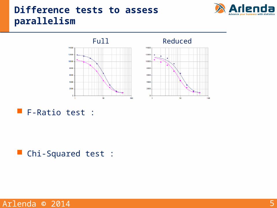
Difference tests to assess parallelism
F-Ratio test :
Chi-Squared test :
Full Reduced
6Arlenda © 2014
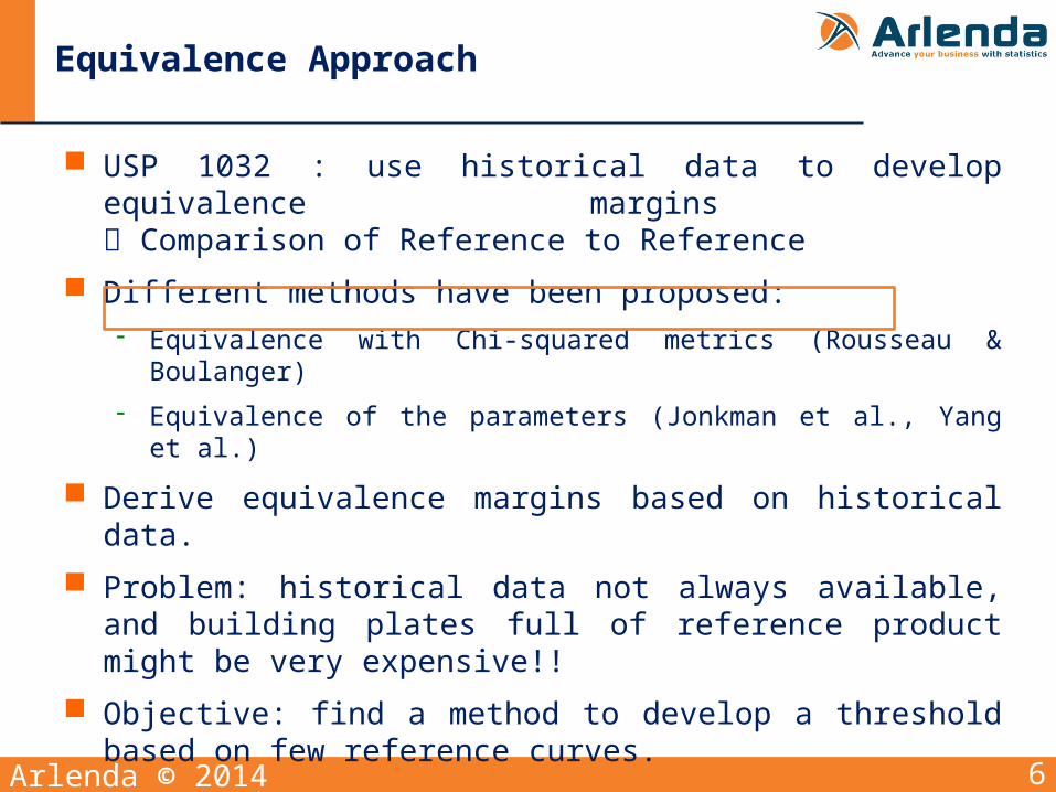
Equivalence Approach
USP 1032 : use historical data to develop equivalence margins Comparison of Reference to Reference
Different methods have been proposed:- Equivalence with Chi-squared metrics (Rousseau & Boulanger)
- Equivalence of the parameters (Jonkman et al., Yang et al.)
Derive equivalence margins based on historical data.
Problem: historical data not always available, and building plates full of reference product might be very expensive!!
Objective: find a method to develop a threshold based on few reference curves.
7Arlenda © 2014
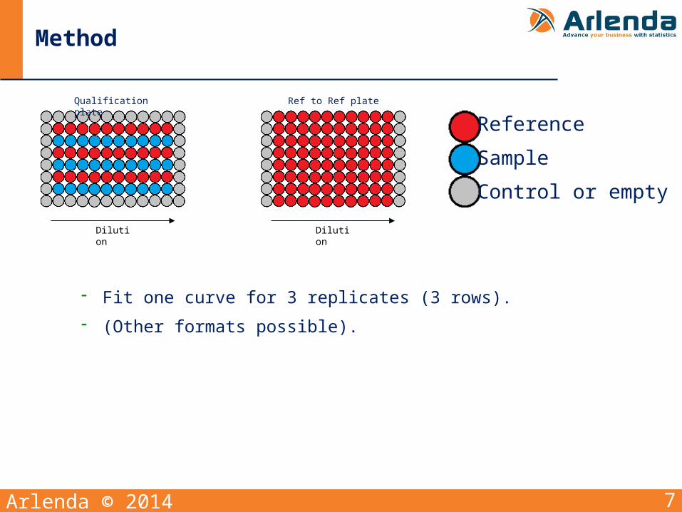
Method
Reference
Sample
Control or empty
Qualification plate Ref to Ref plate
Dilution Dilution
- Fit one curve for 3 replicates (3 rows).
- (Other formats possible).
8Arlenda © 2014
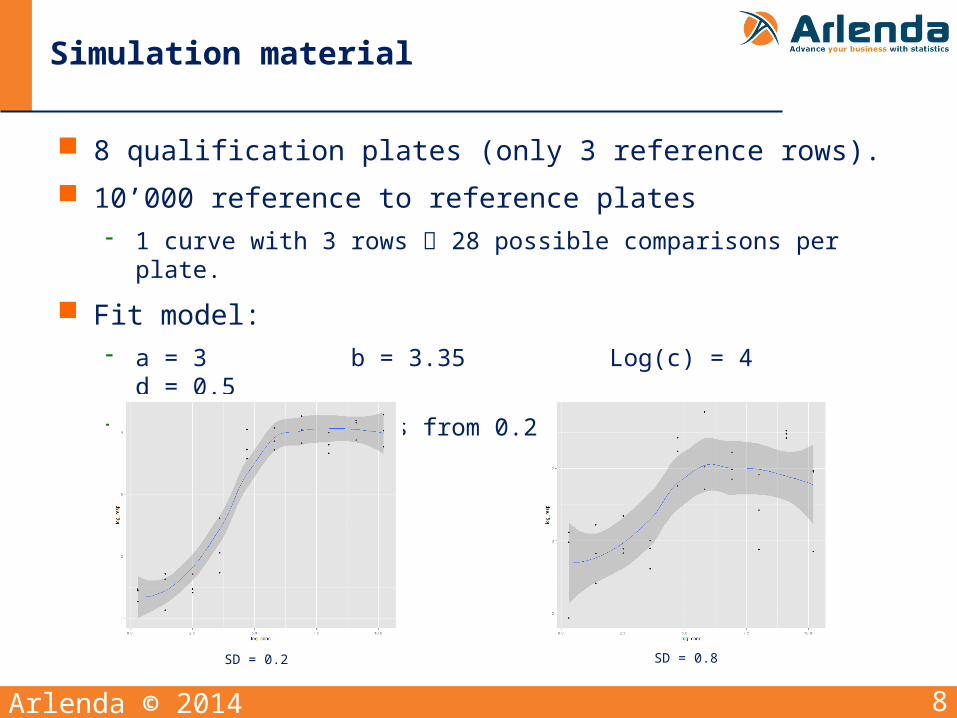
Simulation material
8 qualification plates (only 3 reference rows).
10’000 reference to reference plates- 1 curve with 3 rows 28 possible comparisons per plate.
Fit model:- a = 3 b = 3.35 Log(c) = 4 d = 0.5
- Standard deviations from 0.2 to 0.8
SD = 0.2 SD = 0.8
9Arlenda © 2014
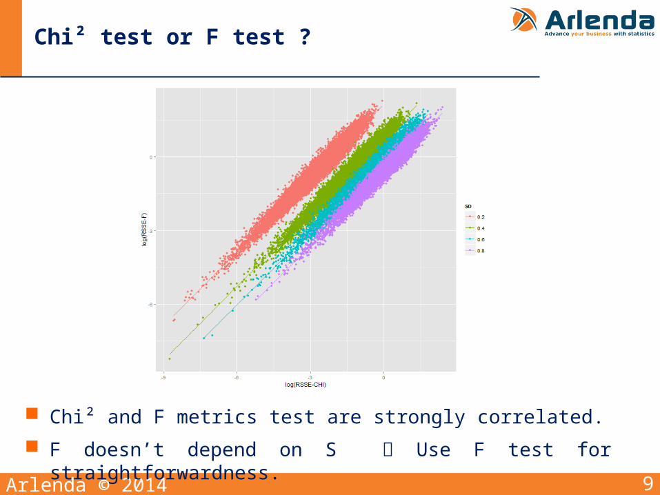
Chi² test or F test ?
Chi² and F metrics test are strongly correlated.
F doesn’t depend on S Use F test for straightforwardness.

10Arlenda © 2014
Comparisons to be done
Distribution of using: - 8 reference plates (very expensive).
- 8 qualification plates using Frequentist method based on bootstrap.
- 8 qualification plates using Bayesian method.
- 10’000 reference plates.
Power comparison- Progressively spread the upper asymptote of test product from upper
asymptote of reference product.
- At each “delta from parallelism” level, perform 1000 parallelism tests.
- Compare the probability of rejection of each method.

11Arlenda © 2014
Simulation of reference curves (1)
Frequentist method:- Fit one curve by plate.
- Bootstrap on residuals to simulate large amount of reference rows for each plate.
- Randomly draw 6 rows (2 curves) and compute parallelism metrics. Repeat operation a large amount of time.
- Combine computed parallelism metrics from each plate.
- Get the 95th percentile of the obtained distribution.
- Repeat all above several times to get the distribution of the percentile
Working within each plate separately allows not to take into account the plate to plate variability (which is sometimes huge).

12Arlenda © 2014
Simulation of reference curves (2)
Bayesian method:- Non-linear mixed effect model with random plate effect on one or several
parameters (select best model).
- Use non-informative prior distributions. Software Stan allows to use uniform prior on every parameter.
- Plate to plate variability can be ignored while simulating curves as it has no effect on the parallelism metrics when comparing two curves from the same plate.
- From posterior chains of parameters, draw 6 rows (2 curves) and compute parallelism metrics. Repeat operation a large amount of time.
- Simulate large amount of reference curves based on posterior chains of parameters
- Get the 95th percentile of the obtained distribution.
- Repeat all above several times to get the distribution of the percentile

13Arlenda © 2014
Distribution of the F ratio
0 1 2 3 4
0.0
0.2
0.4
0.6
0.8
1.0
sd = 0.8
F ratio
De
nsi
ty
0 1 2 3 4
0.0
0.2
0.4
0.6
0.8
sd = 0.2
F ratio
De
nsi
ty
Equivalence 10000 plates
Equivalence 8 plates
Bootstrap estimation
Bayesian estimation
• This pictures present the densities of the F ratios computed with each methods for sd = 0.2 and sd = 0.8
• Black vertical line is the “true p95” (95th percentile of F ratio computed with 10’000 equivalence plates)
• Small curves are the distribution of p95 for 8 equivalence plates, bootstrap and Bayesian approximation
14Arlenda © 2014
Power by threshold
0.0 0.5 1.0 1.5 2.0 2.5
0.0
0.2
0.4
0.6
0.8
1.0
Residual Error = 0.8
Delta from parallelism
Pro
ba
bili
ty o
f re
ject
ion
Equiv 10000BootstrapBayes
0.0 0.5 1.0 1.5 2.0 2.5
0.0
0.2
0.4
0.6
0.8
1.0
Residual Error = 0.2
Delta from parallelism
Pro
ba
bili
ty o
f re
ject
ion
Equiv 10000BootstrapBayes
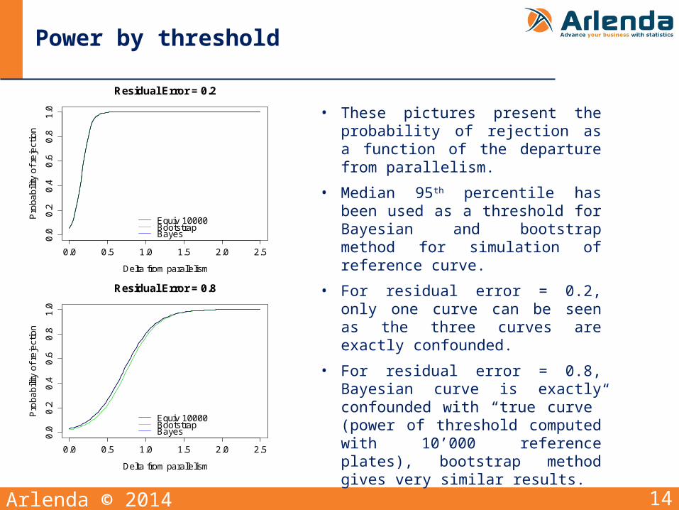
• These pictures present the probability of rejection as a function of the departure from parallelism.
• Median 95th percentile has been used as a threshold for Bayesian and bootstrap method for simulation of reference curve.
• For residual error = 0.2, only one curve can be seen as the three curves are exactly confounded.
• For residual error = 0.8, Bayesian curve is exactly confounded with “true curve” (power of threshold computed with 10’000 reference plates), bootstrap method gives very similar results.

15Arlenda © 2014
Conclusions
With only 8 plates with three rows of reference product, both Bootstrap and Bayesian methods give results that are comparable to the use of 10’000 plates with 8 rows of reference.
These results are both better and much cheaper (in money and time) than building 8 plates full of reference product.
When the residual variability is high, simulation of reference curves using Bayesian method continues to give same results as using 10’000 reference plates.
! Here, we consider homoscedasticity, that’s usually not true, weighting to apply.
16Arlenda © 2014
Ongoing next steps
Define equivalence margins on joint posterior distribution of parameters based on simulated curves.
Perform a power analysis to compare all methods together.
Paper in preparation.
17Arlenda © 2014
Main references
Gottschalk, Paul G., and John R. Dunn. "Measuring parallelism, linearity, and relative potency in bioassay and immunoassay data." Journal of Biopharmaceutical Statistics 15, no. 3 (2005): 437-463.
USP <1032>, “Design and Development of Biological Assays”, 2010.
Rousseau, Réjane and Boulanger, Bruno. “How to develop and assess the parallelism in a bioassays: a fit-for-purpose strategy.” Lecture, European Bioanalysis Forum, Barcelona, 2013.
Yang, Harry et al., “Implementation of Parallelism Testing for Four-Parameter Logistic Model in Bioassays”, PDA J Pharm Sci and Tech, 66(2012): 262-296


