International Journal of Computer Science & Engineering Survey (IJCSES) Vol.6, No.3, June 2015
DOI:10.5121/ijcses.2015.6305 47
EVALUATION OF MIMO SYSTEM CAPACITY OVER
RAYLEIGH FADING CHANNEL
Emad. Mohamed and A.M.Abdulsattar
Alhdba University College, Mousel, Iraq
ABSTRACT
High transmission data rate, spectral efficiency and reliability are essential for future wireless
communications systems. MIMO (multi-input multi-output) diversity technique is a band width efficient
system achieving high data transmission which eventually establishing a high capacity communication
system. Without needing to increase the transmitted power or the channel bandwidth, gain in capacity can
be considerably improved by varying the number of antennas on both sides. Correlated and uncorrelated
channels MIMO system was considered in this paper for different number of antennas and different SNR
over Rayleigh fading channel. At the transmitter both CSI(channel state information) technique and Water
filling power allocation principle was also considered in this paper.
KEYWORDS
Capacity, MIMO, CSI, Rayleigh fading, Water Filling.
1. INTRODUCTION Limits of Channels capacity becomes an important criteria in modern communication system due
to large demand on wireless communication services. In the late 1940s, Claude Shannon
pioneered the channel capacity by developing a mathematical theory of communication based on
the notation of mutual information between the input and output of the transmission channel
[1].The earlier publication in the wireless communications field was considered the capacity of
SISO (single-input single-output), SIMO (single-input multiple-output)and MISO (multiple-input
single-output)over Rayleigh fading channels [2]. SIMO and MISO represents a kind of receiving
and transmitting diversity respectively, where the system capacity logarithmic growth
(bounded) versus number of antennas. During the past few years, Multiple-input multiple-output
(MIMO) has becomes an important subject of research in wireless activities[1].Without
increasing the channel bandwidth or transmitted power, MIMO channel capacity can be
efficiently improved , by adding antenna elements at both transmitter and receiver[3]. This
growing in channel capacity becomes more realistic in the case where there is enough multipath
channels, that is, a rich scattering environment. The main idea behind MIMO system, is its ability
to turn multipath phenomena, traditionally a pitfall of wireless transmission, into a benefit for
increasing system capacity which becomes a promising solution for high bit rate wireless services
[4].The correlation phenomena that appears in MIMO channel is one of the parameters that
strongly affect the system performance. Correlation decreases with an increase in the distance
between antennas, this distance must be not less than � 2� , where � is the signal wave length.
Correlation increasing leads to decreasing in system capacity [5].CSI technique was introduced in
MIMO system for a goal to improve system capacity. The main idea behind CSI technique is to
estimate the channel properties at the transmitter site, which gives a good evaluation for fading
and scattering happened in the communication link. The rest of this paper is organized as follows.

International Journal of Computer Science & Engineering Survey (IJCSES) Vol.6, No.3, June 2015
48
Channel capacity for SISO and different antenna diversity using, SIMO, MISO and MIMO
techniques was presented in section 2. CSI and Equal power allocating criteria was presented in
Sections 3 and 4 respectively. Section 5 provides description of correlated MIMO channel.
Ergodic capacity is introduced in section 6. Finally, a MATLAB simulation results was given in
Section 7.
2. CHANNEL CAPACITY
A communication channel is a medium that is used to transmit signals from a transmitter to a
receiver. During a transmission, the signals at the receiver may be disturbed by noise along with
channel distortions. However, the noise and channel distortions can be differentiated because the
channel distortions are a fixed function applied to the signals while the noise has statistical and
unpredictable perturbations. Let Considering firstly a discrete-time additive white Gaussian noise
(AWGN) channel shown in Figure.1,with a channel input/output relationship represented by (1).
y[t] = x[t] + N[t] (1)
Figure 1. Discrete-time AWGN channel
Assume that it is possible to reliably distinguish M different signal states in a period time of
duration T over a communication channel. Shannon [6–8] showed that if T→∞ the rate of
transmission � approaches the channel capacity � in terms of the number of bits per
transmission.The information (channel) capacity of a Gaussian channel is then represented by(2).
� ≤ � = ��→� ������� �
= 12 ���� �1 + ���
(2)
Where,�� is the signal to noise ratio.
2.1. SISO CAPACITY
For SISO system shown in the Figure2, the capacity is represented by equation (3) [9].
Figure 2.SISO channel

International Journal of Computer Science & Engineering Survey (IJCSES) Vol.6, No.3, June 2015
49
C= log 2(1+ ρ|h|2) bits/s/Hz (3)
Where, h is the normalized complex gain of a fixed wireless channel, ρ is the SNR at the received
antenna.
2.2. SIMO CAPACITY
A block diagram of SIMO channel is shown in the Figure (3).
Figure 3.SIMO channel
SIMO channel mathematical model can be rewritten as:
y = hx+ N (4)
Where h is thenr x 1channel matrix represented by(5).
h = [h1, h2, ...... , hnr]T (5)
Where the elements hi, i= 1, 2,……, nr represents the channel gain between the single transmitter
antenna and the ith receiver antenna over a symbol period, and nr is the received antennas. A
discrete-time SIMO channel capacity is represented by (6) [9]:
(6)
2.3. MISO CAPACITY MISO block diagram is illustrated in the Figure (4).
.
Figure 4.MISO channel
MISO channel mathematical model can be rewritten as:
y = hx+ N (7)

International Journal of Computer Science & Engineering Survey (IJCSES) Vol.6, No.3, June 2015
50
Where h is the 1xntchannel matrix given by (8).
h= [h1, h2, ……, hnt] (8)
And
x = [x1, x2, …… , xnt]T (9)
Where the elements hi, i= 1, 2, ……,nt, represent the constant gain of the channel between the ith
transmitter antenna and the single receiver antenna over a symbol period and nt is the transmitted
antennas. The channel capacity of the discrete-time MISO channel model is represented by
(10)[9].
∁= log� "1 + #$%&|ℎ|�)*+,- ./ 0 12⁄⁄
(10)
2.4. MIMO CAPACITY
MIMO system offers a significant capacity gain over a traditional SISO channel, given that the
underlying channel is rich of scatters with independent spatial fading. MIMO systems offered un
increasing in channel capacity based on the utilization of space (or antenna) diversity at both the
transmitter and the receiver and also on the number of antennas at both sides. A flat fading
communications link was considered in this paper with single user, where the transmitter and
receiver are equipped with nt and nr antennas respectively as shown by Figure 5. The received
signal is represented by (11).
456 = 156756 + $56 (11)
Where, y(i) is the $8 ×1 received signal vector and x(i) is the $* ×1 transmitted signal vector. 156 in (11) is an$8×$* matrix with a complex fading coefficients and its elements assumed to
having an independent and identically distributed (i.i.d) circularly symmetric complex Gaussian
random variables with zero mean and a variance of 1/2 per dimension which leading to a
Rayleigh fading channel model [10].
Also,9:$56$56;< = �=>$8 ,where >$8 denotes the nr x nt identity matrix and9:. < refer to
statistical avarege.
Figure 5. MIMO channel
MIMO system capacity in terms of spectral efficiency i.e. bits per second per Hz, is represented
by (12) [11].
C = Alog�det �EFG + EInKNMHOHP�Q / 0 12⁄⁄ (12)
International Journal of Computer Science & Engineering Survey (IJCSES) Vol.6, No.3, June 2015
51
Where, “det” means determinant, Inr is the nr× nt identity matrix, (·)H means the Hermitian
transpose (or transpose conjugate) and Q is a covariance matrix of the transmitter vector x.
By considering a narrow-band single user MIMO system, the vector notation of the linear link
model between the transmitter and receiver antennas can be represented by (13).
4=Hx+ N (13) Where H is the nr x nt normalized channel matrix, which can be represented as:
R = S ℎ-- ℎ-� … ℎ-)*ℎ�- ℎ�� … ℎ�)*⋮ ⋮ ⋮ ⋮ℎ)8- ℎ)8� … ℎ)8)*V
(14)
Each element hnrnt represents the complex gains between transmitter and the receiver antennas.
3. EQUAL POWER ALLOCATION
Without CSI information at the transmitter, but perfectly known to the receiver, the
optimum power allocation is to divide the available transmit power equally among the
antennas elements of the transmitter. The capacity in (12) can be reduces to a new formula
given by (15), by assuming that the components of the transmitted vector x as statistically
independent, meaning that Q= Int with Gaussian distribution.
C = Alog�det �IFG + EInGNMHHP�Q (15)
It is clear from (15) that the MIMO channel capacity grows linearly for a case ofnr= nt rather than
logarithmically [12,13, 14].
By letting HHH = VDVH (Eigen Value Decomposition theorem), (15) can be reduced to (16)
� = A����XY% �>)8 + 9Z$8�[ \]\;�Q
(16)
Where, 9Z/�[is signal to noise ratio, V is an nr x nr, matrix (eigenvectors of the channel H)
satisfying VHV = VV
H = Inr, and D = diag:�-, ��, … , �+<with. �+ > 0. The MIMO channel
capacity in (16) can be reduces to a new formula represented by (17), based on the fact that
the eigen values (�+) of the channel H was already comprised into the diagonal matrix D.
∁= a&log�Gb,- �1 + EInKNM λb�d ( 17)
Where, r = rank(HHH) = min [$8, $*] (number of parallel channels) and,(i= 1, ... ,r) are the
positive eigen values of HHH.MIMO channel capacity Expressed in (17) represents the sum of the
capacities of r SISO channels, each having power gain,(i= 1, ... ,r) and transmit power Es/nt. It is
noticed that all Eigen channels are allocated the same power; this is because these eigen channels
are not accessible due to the lack of knowledge in the transmitter, i.e. no CSI, so it just divides the
power equally among them [14,15].

International Journal of Computer Science & Engineering Survey (IJCSES) Vol.6, No.3, June 2015
52
4. PERFECT CSI AT THE TRANSMITTER
When CSI technique is applied, the channel matrix H will be feedback to the transmitter from the
receiver, so the transmitter will know the channel matrix here before it transmits the data vectors.
As shown in Figure. 6, the downlink transmitter receives partial CSI feedbacke ′ from the
receiver.
The true channel matrix, which the transmitter does not fully know, can modeled as a Gaussian
random matrix (or vector) who's mean and covariance is given in the feedback [16]. In this case
of action , MIMO system capacity can be improved based on using water filling principle,
through assigning different levels of transmit power to various transmitting antennas [17].
Figure 6. CSI system configuration
Water filling principle is an optimum solution related to a channel capacity improvement. It can
be used to maximize the MIMO channel capacity through allocating of more power to the
transmitted channels that are in good condition and less or none at all to the bad channels.
The capacity of an nr×nt MIMO channel with perfect CSI at the transmitter is represented by
(18)[17].
�fgh�516 = �i7jkl=:�8:k<,- ����XY%no)8 + #1p1;q (18)
Where # is a signal to noise ratio.
To obtain the optimum input covariance matrix (Q=Q*),the transmission is first decoupled along
the individual channel modes, so that n parallel data channels are formed in the directions of the
singular vectors of the channel matrix Hat both the transmitter and the receiver. Along these
modes, deriving Q*requires to find the optimal power allocation {p1,…,pn}and express Q*as: p∗ = \;Xi�:�-∗, … , �)∗<\;; (19)
Here VH is given by the SVD of H 1 = s;∑;\;; (20)
and∑ H= diag{σ1, . . . , σn}, anduv� ≜ �x ≜ �x5y6with W = HHH(for nt>nr) or
W = HHH(for nt<nr), then the MIMO channel capacity under perfect CSI, can be represented by
(21).
�fgh�516 = �i7j:�x<z{|} &����n1 + #�x�xq)v,-
(21)

International Journal of Computer Science & Engineering Survey (IJCSES) Vol.6, No.3, June 2015
53
=∑x,-) ����n1 + #�x∗�xq
The optimum powers allocated are:�-∗, …… , �)∗<, ~ℎ�ℎresulting from applying the well-known
water-filling algorithm.
5. CORRELATED MIMO CHANNELS The most fundamental technique to achieve diversity is to separate sufficiently more than one
antenna from each other so that the relative phases of the multipath contributions are significantly
different at the two adjacent antennas. When large phase differences are present between the total
signals received at each of the antennas, this indicates that there is a low correlation between the
signals at the antennas. Correlation factor decreases with increase in the distance between the
antennas and this distance must be not less than � 2� .More details concerning the effect of
correlation on MIMO channel capacity can be found in reference [18]. Rayleigh correlated
channel was considered here and was represented by (22), using Kronecker model[19].
1� = �8|�1++��*|� 5226
Where1�is the correlated channel matrix, Rr is the receive correlation matrix, Rtis the transmit
correlation matrix, and 1++� is the uncorrelated channel matrix. MIMO system capacity
considering correlated channel is represented by (23). C = EP Alog�det �IFG + EInKNMH�QH�P �Q 5236
6. ERGODIC CAPACITY By taking the ensemble average of the information rate over the distribution of the elements of
the channel matrix H, we obtain the ergodic capacity of a MIMO channel. This capacity is
represented by (24) [20]. �̅ = 9:>< (24)
Without CSI information at the transmitter, the MIMO ergodic capacity is represented by (25).
∁�= 9 �log �XY% �> + �$% 11;��� 5256
With the presents of CSI information at the transmitter, MIMO ergodic capacity is represented by
(26).
�̅ = 9 �& ����n1 + #�x∗�xq)x,- �5266
Where,�xis the singular values of matrix Hand �v∗ is the power coefficient that corresponds to the
amount of power assigned to the kthsub-channel. This coefficient is represented by (27).
�v∗ = 9:|0v|�< (27)

International Journal of Computer Science & Engineering Survey (IJCSES) Vol.6, No.3, June 2015
54
7. SIMULATION AND RESULTS
MIMO channel capacity over Rayleigh fading channel was simulated using MATLAB software
for different antenna configurations, different SNR, uncorrelated and correlated channel (different
correlation coefficients), and with and without CSI. It is found difficult to derive the closed-form
expression for MIMO capacity to plot these capacity versus SNR, therefore Monte Carlo
simulation is used, i.e., a large number around (1000) of random matrices His generated, and then
the average of capacity5�̅6 is taken, by using a software packege for this purpose.
7.1. Uncorrelated and Equal Power
Figure.7 shows the results for uncorrelated channel, where the system capacity is simulated
for SIMO, MISO and MIMO as a function of antennas number at 5dB SNR, for transmitter
diversity MISO and receiver diversity SIMO, capacity leading to logarithmic growth
(bounded).In MIMO system the capacity is linearly growing and much more considerable
than MISO and SIMO systems.
Figure.7 The capacity for MIMO, SIMO, and MISO structures
Figure.8 depicts MIMO capacity for different antenna configurations as a function of SNR. It is
clearly show that the capacity will increase with increasing SNR and also with the numbers of
(ntx nr).

International Journal of Computer Science & Engineering Survey (IJCSES) Vol.6, No.3, June 2015
55
Figure 8.Capacity of different MIMO antenna configurations versus the SNR in dB
Figure 9 show the MIMO capacity variation with (nt x nr) for different values of SNR. It can be
seen that for (5x5) channel the capacities becomes 2, 9 and 19 bit/s/Hz for SNR 0,10 and 20 dB
respectively ,while for(8x8) the capacities becomes 4,18 and 36 respectively ,i.e., multiply by
factor of 2.
Figure 9.MIMO capacity for different SNR-dB versus number of antenna
7.2. Uncorrelated Mimo Channel With Csi
The effect of Channel State Information (CSI) at the transmitter on the overall channel
capacity, with water filling (wf) algorithm to allocate the power among the transmitter
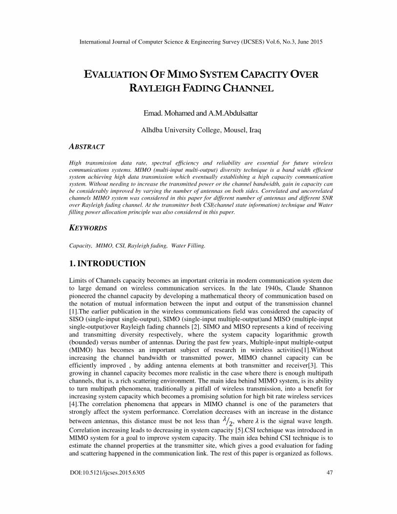
antennas, was investigated here and shown in Figures 10 and 11.
To improvement the capacity by performing wf, is considerable for low SNR=3 dB and a
large number of transmit or received antennas. Figure 10 show that by varying the number of
the receiving antenna a limited gain in the capacity is obtained when fixing the number of the
transmitting antenna.
International Journal of Computer Science & Engineering Survey (IJCSES) Vol.6, No.3, June 2015
56
Figure 10.MIMO capacity with varying nrand nt= 4, SNR = 3 dB
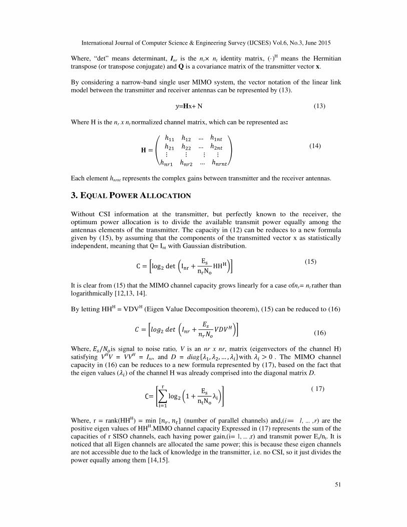
Figure 11 show that by varying the number of the transmitting antenna a considerable gain in the
system capacity is obtained when fixing the number of the receiving antenna.
Figure 11.MIMO capacity with varying ntand nr= 4, SNR = 3 dB
Figure.12 shows the variation of capacity with correlation coefficients(r) for (4x4) channel at 5dB
SNR. By decreasing the distance between antennas, correlation coefficient will increase, leading
to decreasing in system capacity, but still we have considerable gain in case of CSI.
4 5 6 7 8 9 106
7
8
9
10
11
12
Received Ant (nr)
cap
acit
y b
/s/H
z
4xnr wf 5dB
4xnr nowf
4 5 6 7 8 9 106
7
8
9
10
11
12
transmit Ant nt
cap
acit
y b
/s/H
z
ntx4 wf 5dB
ntx4 nowf

International Journal of Computer Science & Engineering Survey (IJCSES) Vol.6, No.3, June 2015
57
Figure 12. (4*4) MIMO channel capacity variation with correlation coefficients(r) at SNR=5dB
8. CONCLUSION
MIMO system capacity was investigated here for different system parameters using MATLAB
software simulation. Simulation result shows that MIMO system has a considerable benefit in
capacity compared with SIMO and MISO system. System capacity was considered for different
MIMO system configuration at both transmitter and receiver by varying the number of antennas.
Simulations results show that the capacity was improved when CSI information was known at the
transmitter by applying Water Filling algorithm. By varying the number of the transmitting
antenna a considerable gain in the system capacity is obtained when fixing the number of the
receiving antenna. Finally, results shows that MIMO channel capacity will decrease when the
correlated factor increase, but still we have a considerable gain in case when applying CSI
technique.
REFERENCES
[1] R.Gray and D.Ornstein, “Block coding for discrete stationary -continuous noisy channels,”
Information Theory, IEEE Transactions on, vol. 25, no. 3, pp. 292 – 306, may 1979.
[2] I.E.Telatar, “Capacity of multi-antenna gaussian channels.” tech. rep., AT & TBell.
[3] P.Sunil Kumar, M.G.Sumithra, M.Sarumathi, " Performance Evaluation of Antenna Selection
Techniques to Improve the Channel Capacity in MIMO Systems," Department of ECE, Bannari
Amman Institute of technology, Tamil Nadu, India, July 2-3, 2013.
[4] J.H.Winters, B "Optimum combining in digital mobile radio with co-channel interference", IEEE J.
Sel. Areas Commun, vol. SAC-2, no. 4, pp. 528–539, Jul.1984.
[5] C.N.Chuah, D. N.C.Tse, and J.M.Kahn, ”Capacity scaling inMIMO wireless systems under correlated
fading”, IEEE Transactions inInformation Theory, vol.48, No. 3, pp. 637-659, March 2002.
[6] Shannon, C.E., “A Mathematical Theory of Communications,” Bell Systems Technology Journal,
Vol. 27, pp. 379–423, July 1948.
[7] Shannon, C.E., “A Mathematical Theory of Communications,” Bell Systems Technology Journal,
Vol. 27, pp. 623–656, October 1948.
[8] Shannon, C.E., “Communication in the Presence of Noise,” Proceedings of the IEEE, Vol. 86, No. 2,
pp. 447–457, February 1998 (this paper is reprinted from the proceedings of the IRE, Vol. 37, No. 1,
pp. 10–21, January 1949).
[9] Gesbert, D., et al., “From Theory to Practice: An Overview of MIMO Space-Time Coded Wireless
Systems,” IEEE Journal on Selected Areas in Communications, Vol.21, No. 3, pp. 281–302, April
2003.

International Journal of Computer Science & Engineering Survey (IJCSES) Vol.6, No.3, June 2015
58
[10] Laxminarayana S. Pillutla and Sudharman K. Jayaweera," Capacity of MIMO Systems in Rayleigh
Fading with Sub-Optimal Adaptive Transmission Schemes" Department of Electrical and Computer
Engineering Wichita State University. October 10–13, 2004
[11] Int. J.Communications, Network and System Sciences, 2010, 3, 213-252
doi:10.4236/ijcns.2010.33031 blished Online March 2010 (http://www.SciRP.org/journal/ijcns/).
[12] Telatar, I.E., “Capacity of Multi-antenna Gaussian Channels,” European Transactionson
Communications, Vol. 10, No. 6, pp. 585–595, 1999.
[13] Foschini, G.J., “Layered Space-Time Architecture for Wireless Communication in a Fading
Environment When Using Multi-Element Antennas,” Bell Labs TechnicalJournal, pp. 41–59, autumn
1996.
[14] Foschini, G.J., et al., “Analysis and Performance of Some Basic Space-Time Architectures,” IEEE
Journal on Selected Areas in Communications, Vol. 21, No.3,pp. 303–320, April 2003.
[15] XiwuLv, Kaihua Liu, Yongtao Ma, " Some results on the capacity of MIMO Rayleigh fading
channels." School of Electronic and Information EngineeringTianjin UniversityTianjin, China.
[16] F. Khalid and J. Speidel, "Advances in MIMO Techniques for Mobile Communications—A Survey,"
Int'l J. of Communications, Network and System Sciences, Vol. 3 No. 3, 2010, pp. 213-252.
[17] Claude Oestges and B Clerckx, "MIMO Wireless Communications: From Real World Propagation to
Space-Time Code", Elsevier Ltd,pp110-115,2007.
[18] A. Paulraj, R.Nabar, and D.Gore.2003. Introduction to Space-Time Wireless Communications,
Cambridge: Cambridge University Press, Chap. 4.
[19] A. Zelst and J.S. Hammerschmidt. "A single coefficient spatial correlation models for multiple-input
multiple output (MIMO) radio channels", in Proc. URSI XXVIIth General Assembly, 2002.
[20] ArogyaswamiPaulra and RohitNabar ،DhananjayGor."Introduction to space time wireless
communications", Cambridge university, pp.72-75, 2003.
Author
1. Eng. Emad. Mohamed was born in Mousel- Iraq on 1964.Lecturer atAlhdba
University College-Mousel-Iraq. Received BSc degreefrom MTC College-Baghdad-
Iraq in 1987.Received MSc degrees from EMU CyprusState University in
2013.Consultant in wireless communication.
2. Dr.Eng. A.M.Abdulsattar was born in Mousel-Iraq on 1954. Lecturer at
AlhdbaUniversity College-Mousel-Iraq. R&D contribution and consultant in wireless
communication. Received BSc degrees from MTC College/Baghdad in 1977.
Received MSc and Ph.D degrees from ENSAE-France in 1979 and 1983 respectively. From 1983 to 1987
Lecturer at MTC College–Baghdad- Iraq. From 1987 to 2004 Researcher at Industrial sector for
development of Electronic and Communication systems. From 2004 to 2006contribute in development of a
privet sector companies for wireless applications. From 2006 to 2014, Lecturer at Mousel University and
Alhdba university college-Mousel-Iraq. Having many Publications in local and International magazines in
the digital communication sector.


![Measurement of Small-Scale Fading Distributions in a ......“Hyper-Rayleigh” fading, though this occurs only in specific, highly dispersive cases [3]. Rayleigh statistics assumes](https://cdn.vdocument.in/doc/165x107/607791c4063fc447bf4d2f0d/measurement-of-small-scale-fading-distributions-in-a-aoehyper-rayleigha.jpg)


