Exact Identi�cation of Read-once Formulas Using Fixed Points of
Ampli�cation Functions
Sally A. GoldmanDepartment of Computer Science
Washington UniversitySt. Louis, MO 63130
Michael J. KearnsAT&T Bell LaboratoriesMurray Hill, NJ 07974
Robert E. SchapireAT&T Bell LaboratoriesMurray Hill, NJ 07974
March 9, 1992
Abstract
In this paper we describe a new technique for exactly identifying certain classesof read-once Boolean formulas. The method is based on sampling the input-outputbehavior of the target formula on a probability distribution that is determined by the�xed point of the formula's ampli�cation function (de�ned as the probability that a1 is output by the formula when each input bit is 1 independently with probabilityp). By performing various statistical tests on easily sampled variants of the �xed-point distribution, we are able to e�ciently infer all structural information about anylogarithmic-depth formula (with high probability). We apply our results to prove theexistence of short universal identi�cation sequences for large classes of formulas. Wealso describe extensions of our algorithms to handle high rates of noise, and to learnformulas of unbounded depth in Valiant's model with respect to speci�c distributions.
Most of this research was carried out while all three authors were at MIT Laboratory for ComputerScience with support provided by ARO Grant DAAL03-86-K-0171, DARPA Contract N00014-89-J-1988,NSF Grant CCR-88914428, and a grant from the Siemens Corporation. R. Schapire received additionalsupport from AFOSR Grant 89-0506 while at Harvard University. S. Goldman is currently supported inpart by a G.E. Foundation Junior Faculty Grant and NSF Grant CCR-9110108.
1

1 Introduction
In this paper we describe e�cient algorithms for exactly identifying certain classes of read-
once Boolean formulas by observing the target formula's behavior on examples drawn ran-
domly according to a �xed and simple distribution that is related to the formula's ampli�ca-
tion function. The class of read-once Boolean formulas is the subclass of Boolean formulas
in which each variable appears at most once. The ampli�cation function Af (p) for a function
f : f0; 1gn ! f0; 1g is de�ned as the probability that the output of f is 1 when each of the n
inputs to f is 1 independently with probability p. Ampli�cation functions were �rst studied
by Valiant [24] and Boppana [4, 5] in obtaining bounds on monotone formula size for the
majority function.
The method used by our algorithms is of central interest. For several classes of formulas,
we show that the behavior of the ampli�cation function is unstable near the �xed point; that
is, the value of Af(p) varies greatly with a small change in p. This in turn implies that small
but easily sampled perturbations of the �xed-point distribution (that is, the distribution
where each input is 1 with probability p, where Af(p) = p) reveal structural information
about the formula. For instance, a typical perturbation of the �xed-point distribution hard-
wires a single variable to 1 and sets the remaining variables to 1 with probability p.
We apply this method to obtain e�cient algorithms for exact identi�cation of classes of
read-once formulas over various bases. These include the class of logarithmic-depth read-once
formulas constructed with not gates and three-input majority gates (for which the �xed-
point distribution is the uniform distribution), as well as the class of logarithmic-depth read-
once formulas constructed with nand gates (for which the �xed-point distribution assigns 1
to each input independently with probability 1=� � 0:618, where � = (1+p5)=2 is the golden
ratio). Thus, for these classes, since the �xed point of the ampli�cation function is the same
for all formulas in the class, for each class we obtain a simple product distribution under which
the class is learnable. As proved by Kearns and Valiant [16, 13], these same classes of formulas
cannot be even weakly approximated in polynomial time when no restriction is placed on
the target distribution; thus, our results may be interpreted as demonstrating that while
there are some distributions that in a computationally bounded setting reveal essentially no
information about the target formula, there are natural and simple distributions that reveal
all information.
For Boolean read-once formulas (a superset of the class of formulas constructed from
nand gates) there is an e�cient, exact-identi�cation algorithm using membership and equiv-
alence queries due to Angluin, Hellerstein and Karpinski [1, 11]. The class of read-once
majority formulas can also be exactly identi�ed using membership and equivalence queries,
as proved by Hancock and Hellerstein [9] and Bshouty, Hancock, Hellerstein, and Karpin-
ski [6]. Brie y, in the query model, the learner attempts to infer the target formula by asking
2

questions, or queries, of a \teacher." For instance, the learner might ask the teacher what
the formula's output would be for a speci�c assignment to the input variable; this is called a
membership query. On an equivalence query, the learner asks if a given conjectured formula
is equivalent to the target formula
Note that our algorithms' use of a �xed distribution can be regarded as a form of \ran-
dom" membership queries, since this �xed and known distribution can be easily simulated
by making random membership queries. Thus, our algorithms are the �rst e�cient proce-
dures for exact identi�cation of logarithmic-depth majority and nand formulas using only
membership queries. Furthermore, the queries used are non-adaptive in the sense that they
do not depend upon the answers received to previous queries. In contrast, all previous al-
gorithms for exact identi�cation, including the algorithms mentioned above, require highly
adaptive queries. As a consequence, our results can be applied to prove the existence of
polynomial-length universal identi�cation sequences for large classes of formulas; these are
�xed sequences of instances for which every unique formula in the class induces a di�erent
labeling.
We also prove that our algorithms are robust against a large amount of random misclas-
si�cation noise, similar to, but slightly more general than that considered by Sloan [23] and
Angluin and Laird [2]. Speci�cally, if �0 and �1 represent the respective probabilities that an
output of 0 or 1 is misclassi�ed, then a robust version of our algorithm can handle any noise
rate for which �0+�1 6= 1; the sample size and computation time required increase only by an
inverse quadratic factor in j1� �0 � �1j. Again regarding our algorithms as using \random"
membership queries, these are the �rst e�cient procedures performing exact identi�cation
in some reasonable model of noisy queries. Our algorithms can also tolerate a modest rate
of malicious noise, as considered by Kearns and Li [14].
Finally, we present an algorithm that learns any (not necessarily logarithmic-depth)
read-once majority formula in Valiant's model against the uniform distribution. To obtain
this result we �rst show that the target formula can be well approximated by truncating
the formula to have only logarithmic depth. We then generalize our algorithm for learning
logarithmic-depth read-once formulas to handle such truncated formulas. A similar result
also holds for read-once nand formulas of unbounded depth.
The problem of learning Boolean formulas against special distributions has been con-
sidered by a number of other authors. In particular, our technique closely resembles that
used by Kearns et al. [15] for learning the class of read-once formulas in disjunctive normal
form (DNF) against the uniform distribution. A similar result, though based on a di�erent
method, was obtained by Pagallo and Haussler [18]. These results were extended by Hancock
and Mansour [10], and by Schapire [21] as described below.
Also, Linial, Mansour and Nisan [17] used a technique based on Fourier spectra to learn
3

the class of constant-depth circuits (constructed from gates of unbounded fan-in) against
the uniform distribution. Furst, Jackson and Smith [7] generalized this result to learn this
same class against any product distribution (i.e., any distribution in which the setting of each
variable is chosen independently of the settings of the other variables). Verbeurgt [25] gives
a di�erent algorithm for learning DNF-formulas against the uniform distribution. However,
all three of these algorithms require quasi-polynomial (npolylog(n)) time, though Verbeurgt's
procedure only requires a polynomial-size sample.
Finally, Schapire [21] has recently extended our technique to handle a probabilistic gen-
eralization of the class of all read-once Boolean formulas constructed from the usual basis
fand;or;notg. He shows that an arbitrarily good approximation of such formulas can be
inferred in polynomial time against any product distribution.
2 Preliminaries
Given a Boolean function f : f0; 1gn ! f0; 1g, Boppana [4, 5] de�nes its ampli�cation
function Af as follows: Af(p) = Pr[f(X1; . . . ;Xn) = 1], where X1; . . . ;Xn are independent
Bernoulli variables that are each 1 with probability p. The quantity Af(p) is called the
ampli�cation of f at p. Valiant [24] uses properties of the ampli�cation function to prove
the existence of monotone Boolean formulas of size O(n5:3) for the majority function on n
inputs. We denote by D(p) the distribution over f0; 1gn induced by having each variable
independently set to 1 with probability p.
For qj 2 f0; 1g and ij 2 f1; . . . ; ng, 1 � j � r, we write f jxi1 q1; . . . ; xir qr to denote
the function obtained from f by �xing or hard-wiring each variable xij to the value qj. If
each qj = q for some value q, we abbreviate this by f jxi1 ; . . . ; xir q.
In our framework, the learner is attempting to infer an unknown target concept c chosen
from some known concept class C. In this paper, C =Sn�1 Cn is parameterized by the
number of variables n, and each c 2 Cn represents a Boolean function on the domain f0; 1gn.A polynomial-time learning algorithm achieves exact identi�cation of a concept class (from
some source of information about the target, such as examples or queries) if it can infer
a concept that is equal to the target concept on all inputs. A polynomial-time learning
algorithm achieves exact identi�cation with high probability if for any � > 0, it can with
probability at least 1 � � infer a concept that is equal to the target concept on all inputs.
In this setting polynomial time means polynomial in n and 1=�. Our algorithms achieve
exact identi�cation with high probability when the example source is a particular, �xed
distribution.
In the distribution-free or probably approximately correct (PAC) learning model, intro-
duced by Valiant [24], the learner is given access to labeled (positive and negative) examples
4

of the target concept, drawn randomly according to some unknown target distribution D.
The learner is also given as input positive real numbers � and �. The learner's goal is to
output with probability at least 1 � � a hypothesis h that has probability at most � of dis-
agreeing with c on a randomly drawn example from D (thus, the hypothesis has accuracy at
least 1� �). In the case of a randomized hypothesis h, the probability that h disagrees with
c is taken over both the random draw from D and the random coin ips used by h. If such
a learning algorithm exists (that is, a polynomial-time algorithm meeting the goal for any
n � 1, any c 2 Cn, any distribution D, and any �; �), we say that C is PAC-learnable. In this
setting, polynomial timemeans polynomial in n, 1=� and 1=�. In this paper, we are primarily
interested in a variant of Valiant's model in which the target distribution is known a priori
to belong to a speci�c restricted class of distributions. This distribution-speci�c model has
also been studied by Benedek and Itai [3].
In this paper we give e�cient algorithms that with high probability exactly identify the
following classes of formulas:
� The class of logarithmic-depth read-once majority formulas: This class con-
sists of Boolean formulas of logarithmic depth constructed from the basis fmaj;notgwhere a maj gate computes the majority of three inputs, and each variable appears at
most once in the formula. Without loss of generality, we assume all not gates are at
the input level.
� The class of logarithmic-depth read-once positive nand formulas: This is
the class of read-once formulas of logarithmic depth constructed from a basis fnandgwhere a nand gate computes the negation of the logical and of two inputs. Note
that each input appears at most once in the formula and all variables are positive
(unnegated). Observe also that the class of read-once positive nand formulas is equiv-
alent to the class of read-once formulas constructed from alternating levels of or/and
gates, starting with an or gate at the top level, with the additional condition that
each variable is negated if and only if it enters an or gate. This observation is easily
proved by repeated application of DeMorgan's law.
Note that by a symmetry argument we can also handle read-once formulas constructed
over the fnorg basis.
In both cases above, our results depend on the restriction on the fan-in of the gates, as
well as the requirement that only variables (and not constants) appear in the leaves of the
target formula.
Note that because we consider only read-once formulas, there is a unique path from any
gate or variable to the output. We de�ne the level or depth of a gate � to be the number
5

of gates (not including � itself) on the path from � to the output. Thus, the output gate
is at level 0. Likewise, we de�ne the level or depth of an input variable to be the number
of gates on the path from the variable to the output. The depth of the entire formula is
the maximum level of any input, and the bottom level consists of all gates and variables of
maximum depth.
An input xi, or a gate �, feeds a gate �0 if the path from xi or � to the output goes through
�0. If xi or � is an input to �0, then we say that xi or � immediately feeds �0. For any two input
bits xi and xj we de�ne �(xi; xj) to be the deepest gate � fed by both xi and xj. Likewise,
�(xi; xj; xk) is the deepest gate � fed by xi, xj, and xk. We say that a pair of variables xi
and xj meet at the gate �(xi; xj). Also, if �(xi; xj) = �(xi; xk) = �(xj ; xk) = �(xi; xj; xk),
then we say that the variables xi, xj and xk meet at gate �(xi; xj; xk); otherwise, the triple
does not meet in the formula. (Note that this only makes sense if there are gates with more
than two inputs, such as a three-input majority gate.)
All logarithms in this paper are base 2.
3 Exact identi�cation of read-once majority formulas
In this section we use properties of ampli�cation functions to obtain a polynomial-time
algorithm that with high probability exactly identi�es any read-once majority formula of
logarithmic depth from random examples drawn according to a uniform distribution.
This type of formula is used by Schapire [20] in his proof that a concept class is weakly
learnable in polynomial time if and only if it is strongly learnable in polynomial time. That is,
the hypothesis output by his boosting procedure can be viewed as a majority formula whose
inputs are the hypotheses output by the weak learning algorithm. We also note that a read-
once majority formula cannot in general be converted into a read-once Boolean formula over
the usual fand;or;notg basis. (For example, a single three-input majority gate cannot be
converted into a read-once Boolean formula over this basis; this can be proved, for instance,
by enumerating all three-input read-once Boolean formulas.)
It can be shown that the class of logarithmic-depth read-once majority formulas is
not learnable in the distribution-free model, modulo assorted cryptographic assumptions.1
Brie y, this can be proved using a Pitt and Warmuth-style \prediction-preserving reduc-
tion" [19] to show that learning read-once majority formulas is at least as hard as learning
general Boolean formulas. Our reduction starts with a given Boolean formula which we
can assume without loss of generality has been converted using standard techniques into
an equivalent formula of logarithmic depth. The main idea of the reduction is to replace
1Namely, these hardness results depend on the assumed intractability of factoring Blum integers, inverting
RSA functions, and recognizing quadratic residues. See Kearns and Valiant [16] for details.
6
each or gate (respectively, and gate) occurring in this formula with a maj gate, one of
whose inputs is wired to a distinct variable that, under the target distribution, always has
the value 1 (respectively, 0). The resulting majority formula can further be reduced to one
that is read-once using the substitution method of Kearns et al. [15]. Finally, combined with
Kearns and Valiant's result that Boolean formulas are not learnable (modulo cryptographic
assumptions), this shows that majority formulas are also not learnable.
Despite the hardness of this class in the general distribution-free framework, we show
that the class is nevertheless exactly identi�able when examples are chosen from the uniform
distribution. The algorithm consists of two phases. In the �rst phase, we determine the
relevant variables (i.e., those that occur in the formula), their signs (i.e., whether they are
negated or not), and their levels. To achieve this goal, for each variable, we hard-wire its
value to 1 and estimate the ampli�cation of the induced function at 12using examples drawn
randomly from the uniform distribution on the remaining variables. Here, by \hard-wiring"
a variable to 1, we really mean that we apply a �lter that only lets through examples
for which that variable is 1. We prove that if the variable is relevant, then with high
probability this estimate will be signi�cantly smaller or greater than 12, depending on whether
the variable occurs negated or unnegated in the formula; otherwise, this estimate will be near12. Furthermore, the level of a relevant variable can be determined from the amount by which
the ampli�cation of the induced function di�ers from 12 .
In the second phase of the algorithm, we construct the formula. More precisely, we �rst
construct the bottom level of the formula, and then recursively construct the remaining
levels. To construct the bottom level of the formula, we begin by �nding triples of variables
that are inputs to the same bottom-level gate. To do this, for each triple of relevant variables
that have the largest level number, we hard-wire the three variables to 1 and again estimate
the ampli�cation of the induced function from random examples. We show that we can
determine whether the three variables all enter the same bottom-level gate based on this
estimate.
Brie y, the recursion works as follows. When constructing level t of the formula, if we
�nd that xi, xj, and xk are inputs to the same level-t gate, then in the recursive call we
replace xi, xj, and xk by a level-t meta-variable y � maj(xi; xj; xk). Since y is a known
subformula, its output on any example can be easily computed and y can be treated like
an ordinary variable. Furthermore, since 12 is the �xed point for the ampli�cation function
of any read-once majority formula, it follows that y is 1 with probability 12. Thus, for the
recursive call we replace all triples of variables that enter level-t gates with meta-variables,
and we easily obtain our needed source of random examples drawn according to the uniform
distribution on the new variable set from the original source of examples.
For the remainder of this section, we explore some of the properties of the ampli�cation
7

function of read-once majority formulas, leading eventually to a proof of the correctness of
this algorithm.
Lemma 3.1 Let X1, X2 and X3 be three independent Bernoulli variables, each 1 with prob-
ability p1, p2 and p3, respectively. Then Pr[maj(X1;X2;X3) = 1] = p1p2 + p1p3 + p2p3 �2p1p2p3.
Proof: The stated probability is exactly the chance that at least two of the three variables
are 1.
Lemma 3.1 implies that Af (12) = 1
2for any read-once majority formula f . Thus, 1
2is a
�xed point of Af .
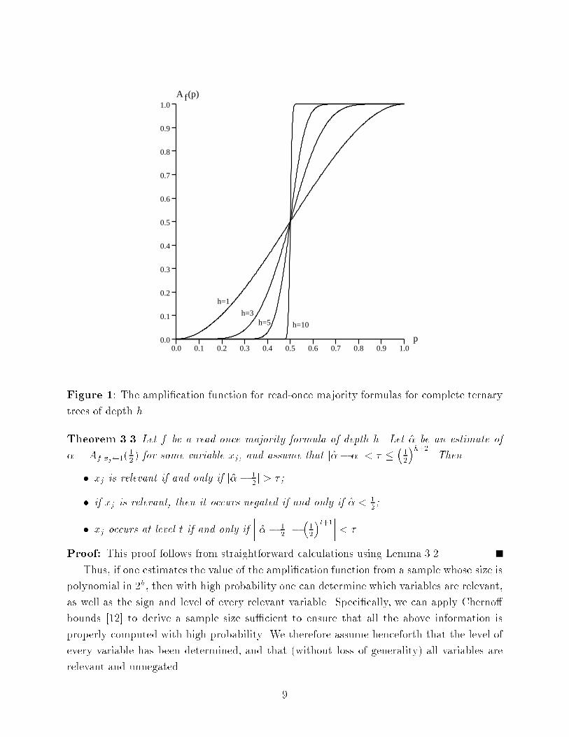
Our approach depends on the fact that the �rst derivative of Af is large at12, meaning
that a slight perturbation of D(1=2) (i.e., the uniform distribution) tends to perturb the
statistical behavior of the formula su�ciently to allow exact identi�cation. See Figure 1
for a graph showing the ampli�cation function for balanced read-once majority formulas of
various depths.
We perturb D(1=2) by hard-wiring a small number of variables to be 1; such perturba-
tions can always be e�ciently sampled by simply waiting for the desired variables to be
simultaneously set to 1 in a random example from D(1=2).
We begin by considering the e�ect on the function's ampli�cation of altering the proba-
bility with which one of the variables xj is set to 1. This will be important in the analysis
that follows.
Lemma 3.2 Let f be a read-once majority formula, and let t be the level of an unnegated
variable xj. Then for q 2 f0; 1g, Af jxj q(12) =
12 +
�12
�t(q � 1
2).
Proof: By induction on t. When t = 0, the formula consists just of the variable xj, and the
lemma holds. For the inductive step, let f1, f2 and f3 be the functions computed by the three
subformulas obtained by deleting the output gate of f ; thus, f is just the majority of f1,
f2 and f3. Note that xj occurs in exactly one of these three subformulas|assume it occurs
in the �rst. Since xj occurs at level t � 1 of this subformula, by the inductive hypothesis,
Af1jxj q(12) = 1
2 +�12
�t�1(q � 1
2), and since xj does not occur in the other subformulas,
Afijxj q(12) =
12 for i = 2; 3. From Lemma 3.1, it follows that Af jxj q(
12) has the stated
value, completing the induction.
It can now be seen how we use the ampli�cation function to determine the relevant
variables of f : if xj is relevant, then the statistical behavior of the output of f changes
signi�cantly when xj is hard-wired to 1. Similarly, the sign and the level of each variable
can be readily determined in this manner.
8
0.0 0.1 0.2 0.3 0.4 0.5 0.6 0.7 0.8 0.9 1.00.0
0.1
0.2
0.3
0.4
0.5
0.6
0.7
0.8
0.9
1.0
p
A (p)f
h=1
h=3h=5 h=10
Figure 1: The ampli�cation function for read-once majority formulas for complete ternary
trees of depth h.
Theorem 3.3 Let f be a read-once majority formula of depth h. Let �̂ be an estimate of
� = Af jxj 1(12) for some variable xj, and assume that j�̂� �j < � �
�12
�h+2. Then
� xj is relevant if and only if j�̂ � 12j > � ;
� if xj is relevant, then it occurs negated if and only if �̂ < 12;
� xj occurs at level t if and only if����j�̂ � 1
2 j ��12
�t+1���� < � .
Proof: This proof follows from straightforward calculations using Lemma 3.2.
Thus, if one estimates the value of the ampli�cation function from a sample whose size is
polynomial in 2h, then with high probability one can determine which variables are relevant,
as well as the sign and level of every relevant variable. Speci�cally, we can apply Cherno�
bounds [12] to derive a sample size su�cient to ensure that all the above information is
properly computed with high probability. We therefore assume henceforth that the level of
every variable has been determined, and that (without loss of generality) all variables are
relevant and unnegated.
9

More problematic is determining exactly how the variables are combined in f . A natural
approach is to try hard-wiring pairs of variables to 1, and to again estimate the ampli�cation
of the induced function in the hopes that some structural information will be revealed. The
following lemma, that is useful at a later point, shows that this approach fails.
Lemma 3.4 Let f be a read-once majority formula, and let xi and xj be distinct, unnegated
variables that occur at levels t1 and t2, respectively. Then
Af jxi;xj 1(12) = 1
2+�12
�t1+1+�12
�t2+1;
regardless of the depth d of � = �(xi; xj).
Proof: By induction on d. Let f1, f2 and f3 be the three subformulas of f that are inputs
to the output gate so that f = maj(f1; f2; f3).
If d = 0, then � is the output gate, and xi and xj occur in two of the subformulas (say,
f1 and f2, respectively). From Lemma 3.2, it follows that
Afkjxi;xj 1(12) = 1
2+�12
�tk
for k = 1; 2, and, since neither xi nor xj is relevant to f3, Af3jxi;xj 1(12) = 1
2. The stated
value for Af jxi;xj 1(12) follows then from Lemma 3.1.
If d > 0, then � is a gate occurring in one of the subformulas (say f1) at level d � 1 of
the subformula. By inductive hypothesis,
Af1jxi;xj 1(12) = 1
2+�12
�t1+�12
�t2:
Also, Afkjxi;xj 1(12) = 1
2for k = 2; 3. The stated value for Af jxi;xj 1(
12) again follows from
Lemma 3.1.
Thus, if two relevant variables are hard-wired to 1, no information is obtained by knowing
the value of the ampli�cation function. That is, the ampli�cation function is independent of
the level at which the two variables meet.
Therefore, we instead consider what happens when three relevant variables of the same
level are �xed to 1. In fact, it turns out to be su�cient to do so for triples of variables all of
which occur at the bottom level of the formula. We show that by doing so one can determine
the full structure of the formula.
For each triple xi, xj and xk all occurring at level t, there are essentially two cases to
consider; either
1. the triple xi, xj, xk does not meet in the formula; or
2. the three variables xi, xj and xk meet at the gate �(xi; xj; xk). We divide this case
into two sub-cases:
10
(a) xi, xj and xk are inputs to the same gate so that �(xi; xj; xk) occurs at level t�1;or
(b) �(xi; xj; xk) occurs at some level d < t� 1.
We are interested in separating Case 2a from the other cases by estimating the ampli�cation
of the function when all three variables are hard-wired to 1. This is su�cient to reconstruct
the structure of the formula: if we can �nd three variables that are inputs to some gate �
(and there always must exist such a triple), then we can essentially replace the subformula
consisting of the three variables and the gate � by a new meta-variable whose value can
easily be determined from the values of the original three variables. Furthermore, since 12
is a �xed point for all read-once majority formulas the meta-variables' statistics will be the
same as those of the original variables. Thus, the total number of variables is reduced by
two, and the rest of the formula's structure can be determined recursively.
The following two lemmas analyze the ampli�cation of the function when three variables
are hard-wired to 1 in both of the above cases. We begin with Case 2:
Lemma 3.5 Let f be a read-once majority formula. Let xi, xj and xk be three distinct,
unnegated inputs that occur at levels t1, t2 and t3, respectively, and which meet at gate
� = �(xi; xj; xk). Let d be the level of �. Then
Af jxi;xj;xk 1(12) = 1
2+�12
�t1+1+�12
�t2+1+�12
�t3+1 � �12
�t1+t2+t3�2d�1:
Proof: By induction on d. As in the preceding lemmas, suppose that f = maj(f1; f2; f3).
If d = 0, then � is the output gate of f , and, without loss of generality, xi, xj and xk occur
one each in f1, f2 and f3, respectively. From Lemma 3.2, Afr jxi;xj;xk 1(12) = 1
2+�12
�tr, for
r = 1; 2; 3. The stated value for Af jxi;xj;xk 1(12) follows from Lemma 3.1.
If d > 0, then one of the subformulas (say, f1) contains � at depth d � 1. By inductive
hypothesis,
Af1jxi;xj ;xk 1(12) = 1
2+�12
�t1+�12
�t2+�12
�t3 � �12
�t1+t2+t3�2d�2;
and of course, Afrjxi;xj;xk 1(12) = 1
2for r = 2; 3. The proof is completed by again applying
Lemma 3.1.
So, unlike the situation in which only two variables are hard-wired to 1, here the value of
the ampli�cation function depends on the level of the formula at which the three variables
meet. However, it may be the case that xi, xj, and xk do not meet at all (i.e., we may be in
Case 1). The next lemma considers this case.
11

Lemma 3.6 Let f be a read-once majority formula. Let xi, xj and xk be three distinct,
unnegated inputs that occur at levels t1, t2 and t3, respectively, and for which �0 = �(xi; xj) 6=�(xi; xj; xk) = �. Then
Af jxi;xj;xk 1(12) = 1
2+�12
�t1+1+�12
�t2+1+�12
�t3+1;
regardless of the levels d and d0 of gates � and �0.
Proof: By induction on d. As before, assume that f = maj(f1; f2; f3). If d = 0, then � is
the output gate, �0 occurs (say) in f1, and xk in f2. From Lemma 3.4, Af1jxi;xj;xk 1(12) = 1
2+�
12
�t1+�12
�t2, and from Lemma 3.2, Af2jxi;xj;xk 1(
12) = 1
2+�12
�t3. Also, Af3jxi;xj;xk 1(
12) = 1
2.
Lemma 3.1 then implies the stated value for Af jxi;xj;xk 1(12).
If d > 0, then � occurs, say, in f1. By inductive hypothesis, Af1jxi;xj;xk 1(12) = 1
2+�12
�t1+�
12
�t2+�12
�t3, and clearly Afrjxi;xj;xk 1(
12) =
12 for r = 2; 3. An application of Lemma 3.1
completes the induction.
Combining these lemmas, we can show that Case 2a can be separated from the other
cases by estimating the function's ampli�cation with triples of variables hard-wired to 1.
Theorem 3.7 Let f be a read-once majority formula. Let xi, xj and xk be three distinct,
unnegated, level-t inputs. Let �̂ be an estimate of � = Af jxi;xj;xk 1(12) for which j�̂��j < � �
3�12
�t+4. Then xi, xj and xk are inputs to the same gate of f if and only if �̂ < 1
2+�12
�t+� .
Proof: If Case 2a applies, then Lemma 3.5 implies that � = 12 +
�12
�t. Otherwise, if either
Case 1 or 2b applies, then Lemmas 3.5 and 3.6 imply that � � 12+�12
�t+ 3
�12
�t+3. The
theorem follows immediately.
We are now ready to state the main result of this section:
Theorem 3.8 There exists an algorithm with the following properties: Given h, n, � >
0, and access to examples drawn from the uniform distribution on f0; 1gn and labeled by
any read-once majority formula f of depth at most h on n variables, the algorithm exactly
identi�es f with probability at least 1 � �. The algorithm's sample complexity is O(4h �log(n=�)), and its time complexity is O(4h � (r3 + n) � log(n=�)), where r is the number of
relevant variables appearing in the target formula.
Proof: First, for each variable xi, estimate the function's ampli�cation with xi hard-wired
to 1. (We will ensure that, with high probability, this estimate is within�12
�h+2of the true
ampli�cation.) It follows from Theorem 3.3 that after this phase of the algorithm, with high
probability we know which variables are relevant, and the sign and depth of each relevant
variable. (So, we assume from now on that the formula is monotone.)
12

In the second phase of the algorithm, we build the formula level by level from bottom to
top. To build the bottom level, for all triples of variables xi, xj, xk that enter the bottom
level, we estimate the ampli�cation with xi, xj, and xk hard-wired to 1. (We will ensure that,
with high probability, this estimate is within 3�12
�h+4of the true ampli�cation.) It follows
from Theorem 3.7 that we can determine which variables enter the same bottom-level gates.
We want to recurse to compute the other levels; however, we cannot hard-wire too many
variables without the �lter requiring too many examples. The key observation is that on
examples drawn from the uniform distribution, the output of any subformula is 1 with
probability 12. Thus, the inputs into any level are in fact distributed according to a uniform
distribution. Since we compute the formula from bottom to top, the �lter can just compute
the value for the known levels to determine the inputs to the level currently being learned.
Our algorithm is described in Figure 2.
Given that the estimates for the formula's ampli�cation have the needed accuracy, the
proof of correctness follows from Theorems 3.3 and 3.7. To compute the actual sample size
needed to make these estimates, we use Hoe�ding's inequality [12] (also known as a form of
Cherno� bounds) as stated below:
Lemma 3.9 (Hoe�ding's Inequality) Let X1; . . . ;Xm be a sequence of m independent
Bernoulli trials, each succeeding with probability p. Let S = X1 + � � � + Xm be the random
variable describing the total number of successes. Then for 0 � � 1, the following holds:
Pr[jS � pmj > m] � 2e�2m 2
:
In the �rst phase of the algorithm, for each variable xi, we need a good estimate �̂ of
� = Af jxi 1(12); speci�cally, we require that the chosen sample be su�ciently large that
j�� �̂j < 2�(h+2) with probability at least 1 � �=2n. Then every such estimate for the n
variables will have the needed accuracy with probability at least 1 � �=2.Using Hoe�ding's inequality it can be shown that a �ltered sample (i.e., the sample after
all examples are removed for which xi = 0) of size m1 > 8 � 4h ln(8n=�) is su�ciently large
to ensure that the estimate �̂ has the needed accuracy with probability at least 1 � �=4n.Again using Hoe�ding's inequality, it can be shown that if we draw an (un�ltered) sample
of size at least maxf4m1; 8 ln(4=�)g then with probability at least 1 � �=4n, at least 1=4 of
the examples chosen will be such that xi = 1, and thus, the �ltered sample will have size at
least m1. So by using a sample of size exceeding 32 � 4h ln(8n=�), all of the estimates satisfy
the requirements for the �rst phase of the algorithm with probability at least 1� �=2.In the second phase, we require good estimates of the formula's ampli�cation when triples
of variables are hard-wired. In fact, we need such estimates not only when ordinary variables
are hard-wired, but also when we hard-wire meta-variables. Note that, assuming all estimates
have the needed accuracy, every (meta-)variable added to the set X in Figure 2 in fact
13
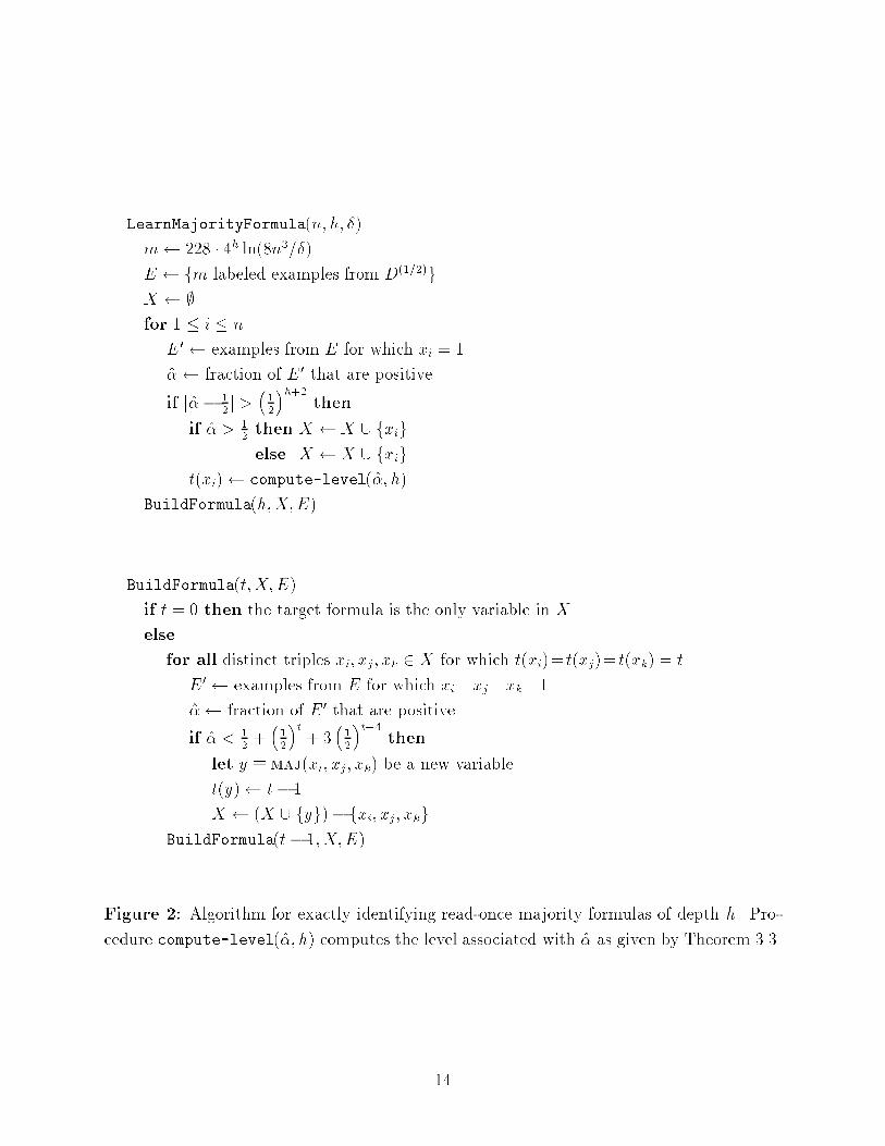
LearnMajorityFormula(n; h; �)
m 228 � 4h ln(8n3=�)E fm labeled examples from D(1=2)gX ;for 1 � i � n
E0 examples from E for which xi = 1
�̂ fraction of E0 that are positive
if j�̂� 12j >
�12
�h+2then
if �̂ > 12then X X [ fxigelse X X [ f�xig
t(xi) compute-level(�̂; h)
BuildFormula(h;X;E)
BuildFormula(t;X;E)
if t = 0 then the target formula is the only variable in X
else
for all distinct triples xi; xj; xk 2 X for which t(xi)= t(xj)= t(xk) = t
E 0 examples from E for which xi=xj=xk=1
�̂ fraction of E0 that are positive
if �̂ < 12 +
�12
�t+ 3
�12
�t+4then
let y � maj(xi; xj; xk) be a new variable
t(y) t� 1
X (X [ fyg)� fxi; xj; xkgBuildFormula(t� 1;X;E)
Figure 2: Algorithm for exactly identifying read-once majority formulas of depth h. Pro-
cedure compute-level(�̂; h) computes the level associated with �̂ as given by Theorem 3.3.
14
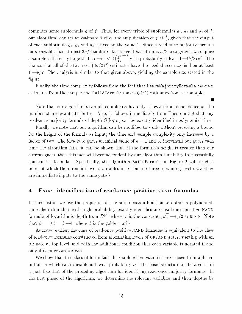
computes some subformula g of f . Thus, for every triple of subformulas g1, g2 and g3 of f ,
our algorithm requires an estimate �̂ of �, the ampli�cation of f at 12, given that the output
of each subformula g1, g2 and g3 is �xed to the value 1. Since a read-once majority formula
on n variables has at most 3n=2 subformulas (since it has at most n=2 maj gates), we require
a sample su�ciently large that j�� �̂j < 3�12
�h+4with probability at least 1�4�=27n3. The
chance that all of the (at most (3n=2)3) estimates have the needed accuracy is then at least
1 � �=2. The analysis is similar to that given above, yielding the sample size stated in the
�gure.
Finally, the time complexity follows from the fact that LearnMajorityFormulamakes n
estimates from the sample and BuildFormula makes O(r3) estimates from the sample.
Note that our algorithm's sample complexity has only a logarithmic dependence on the
number of irrelevant attributes. Also, it follows immediately from Theorem 3.8 that any
read-once majority formula of depth O(log n) can be exactly identi�ed in polynomial time.
Finally, we note that our algorithm can be modi�ed to work without receiving a bound
for the height of the formula as input; the time and sample complexity only increase by a
factor of two. The idea is to guess an initial value of h = 1 and to increment our guess each
time the algorithm fails; it can be shown that, if the formula's height is greater than our
current guess, then this fact will become evident by our algorithm's inability to successfully
construct a formula. (Speci�cally, the algorithm BuildFormula in Figure 2 will reach a
point at which there remain level-t variables in X, but no three remaining level-t variables
are immediate inputs to the same gate.)
4 Exact identi�cation of read-once positive nand formulas
In this section we use the properties of the ampli�cation function to obtain a polynomial-
time algorithm that with high probability exactly identi�es any read-once positive nand
formula of logarithmic depth from D( ) where is the constant (p5 � 1)=2 � 0:618. Note
that = 1=� = �� 1, where � is the golden ratio.
As noted earlier, the class of read-once positive nand formulas is equivalent to the class
of read-once formulas constructed from alternating levels of or/and gates, starting with an
or gate at top level, and with the additional condition that each variable is negated if and
only if it enters an or gate.
We show that this class of formulas is learnable when examples are chosen from a distri-
bution in which each variable is 1 with probability . The basic structure of the algorithm
is just like that of the preceding algorithm for identifying read-once majority formulas. In
the �rst phase of the algorithm, we determine the relevant variables and their depths by
15

hard-wiring each variable to 0, and estimating the ampli�cation of the induced function at
using random examples from D( ). In the second phase of the algorithm, we construct the
formula by �nding pairs of variables that are direct inputs to a bottom-level gate. Here, we
show that this is possible by hard-wiring pairs of variables to 0 and estimating the function's
ampli�cation. After learning the structure of the bottom level of the formula, we again are
able to construct the remaining levels recursively.
Since the techniques used in this section are so similar to those in Section 3, the proofs of
the lemmas and theorems have been omitted. Most of the lemmas can be proved by simple
induction arguments as before.
We turn now to a discussion of some of the properties of the ampli�cation function of
read-once positive nand formulas; these lead to a proof of the correctness of our algorithm.
Lemma 4.1 Let X1 and X2 be independent Bernoulli variables, each 1 with probability p1
and p2, respectively. Then Pr[nand(X1;X2) = 1] = 1� p1p2.
It is easily veri�ed that 1� 2 = , and thus that is a �xed point of the ampli�cation
function Af whenever f is a read-once positive nand formula. Once again, our approach
depends on the fact that slight perturbations of D( ) tend to perturb the statistical behavior
of the formula su�ciently to allow exact identi�cation.
Lemma 4.2 Let f be a read-once positive nand formula, and let t be the level of some
variable xj. Then Af jxj q( ) = + (q � )(� )t.
Thus, hard-wiring an even-leveled input to 0 decreases the ampli�cation while hard-wiring
an odd-leveled input to 0 increases the ampli�cation. To give some intuition explaining this
behavior, consider the correspondence described above between read-once positive nand
formulas and leveled or/and formulas. An even-leveled input corresponds to an input to an
and gate and thus hard-wiring that input to 0 clearly decreases the ampli�cation. However,
an odd-leveled input corresponds to an input that is �rst negated and then fed to an or
gate; thus, this case corresponds to hard-wiring the input to an or gate to 1 which clearly
increases the ampli�cation function.
As we saw in the last section, the ampli�cation function can be used to determine the
relevant variables of f : if xj is relevant then the statistical behavior of the output of f
changes signi�cantly when xj is hard-wired to 0. Similarly, the level of each variable can be
computed in this manner.
Theorem 4.3 Let f be a read-once positive nand formula of depth h. Let �̂ be an estimate
of � = Af jxj 0( ) for some variable xj, and assume that j�̂ � �j < � � h+1=2. Then
� xj is relevant if and only if j�̂ � j > � ;
16

� xj occurs at level t if and only if j + (� )t+1 � �̂j < � .
We next consider the e�ect on the ampli�cation function of hard-wiring two inputs.
Unlike the case of majority formulas, measuring the ampli�cation of the function when pairs
of variables are hard-wired to 0 reveals a great deal of information about the structure of
the formula. In particular, the value of the ampli�cation function when two level-t variables
xi and xj are hard-wired to 0 depends critically on the depth of �(xi; xj).
Lemma 4.4 Let f be a read-once positive nand formula, and let xi and xj be two distinct
variables that occur at levels t1 and t2, respectively, and for which � = �(xi; xj) is at level d.
Then
Af jxi;xj 0( ) = + (� )t1+1 + (� )t2+1 � (� )t1+t2�d:
Using the same ideas as in the last section, it can now be proved that, given a good
estimate of the ampli�cation function, one can determine which variables meet at bottom-
level gates.
Theorem 4.5 Let f be a read-once positive nand formula. Let xi and xj be two level-t
inputs. Let �̂ be an estimate of � = Af jxi;xj 0( ) for which j�̂ � �j < � � t+3=2. Then xi
and xj are inputs to the same level-(t � 1) gate of f if and only if j + (� )t+1 � �̂j < � .
We are now ready to state the main result of this section:
Theorem 4.6 Let = 1=� = (p5�1)=2. Then there exists an algorithm with the following
properties: Given h, n, � > 0, and access to examples drawn from the distribution D( )
on f0; 1gn and labeled by any read-once positive nand formula f of depth at most h on n
variables, the algorithm exactly identi�es f with probability at least 1 � �. The algorithm's
sample complexity is O(�2h � log(n=�)), and its time complexity is O(�2h � (r2+n) � log(n=�)),where r is the number of relevant variables appearing in the target formula.
Our algorithm is obtained bymaking straightforward modi�cations to LearnMajorityFormula
and BuildFormula. The proof that this algorithm is correct follows from the preceding lem-
mas and theorems, and is similar to the proof of Theorem 3.8.
As before, it follows immediately that any read-once positive nand formula of depth at
most O(log n) can be exactly identi�ed in polynomial time.
17

5 Short universal identi�cation sequences
In this section we describe an interesting consequence of our results. Observe that if we regard
our algorithms' use of a �xed distribution as a form of \random" membership queries, then
it is apparent that these queries are non-adaptive; each query is independent of all previous
answers. In other words, our algorithms pick all membership queries before seeing the
outcome of any. From this observation we can apply our results to prove the existence of
polynomial-length universal identi�cation sequences for classes of formulas, that is, �xed
sequences of instances that distinguish all concepts from one another.
More formally, we de�ne an instance sequence to be an unlabeled sequence of instances,
and an example sequence to be a labeled sequence of instances. Let Cn be a concept class.
We say an instance sequence S distinguishes a concept c if the example sequence obtained
by labeling S according to c distinguishes c from all other concepts in Cn; that is, c is theonly concept consistent with the example sequence so obtained. A universal identi�cation
sequence for a concept class Cn is an instance sequence that distinguishes every concept
c 2 Cn.In the language used in the related work of Goldman and Kearns [8], a sequence that
distinguishes c would be called a teaching sequence for c. Thus, in their terminology, a
universal identi�cation sequence is one that acts as a teaching sequence for every c 2 Cn.See also the related work of Shinohara and Miyano [22].
The following theorem gives general conditions for when a deterministic exact identi�ca-
tion algorithm implies the existence of a polynomial-length universal identi�cation sequence.
We then apply this theorem to our algorithms of the previous sections.
Theorem 5.1 Let Cn be a concept class with cardinality jCnj � 2p(n), where p(n) is some
polynomial. Let A be a deterministic algorithm that, given � > 0 and random, labeled
examples drawn from some �xed distribution D, exactly identi�es any c 2 Cn with probability
exceeding 1 � �. Furthermore, suppose that the sample complexity of A is q(n) logk(1=�)
for some polynomial q(n) and constant k. Then there exists a polynomial-length universal
identi�cation sequence for Cn. Speci�cally, there exists such a sequence of length q(n)�(p(n))k.
Proof: The proof uses a standard probabilistic argument. Fix c 2 Cn, and let S be the
random example sequence drawn by algorithm A. Since algorithm A achieves exact iden-
ti�cation of c with probability exceeding 1 � � we have that the probability, taken over all
random example sequences for c, that A fails to exactly identify the particular target concept
c is less than �. Letting � = 2�p(n) it follows that the probability, taken over all random
instance sequences, that A fails to identify any target concept in Cn is less than jCnj� � 1.
Thus, with positive probability, an instance sequence of length q(n)(p(n))k drawn randomly
18
from D causes A to exactly identify any c 2 Cn. Call such a sequence good . Therefore there
must exist some good instance sequence S of this length.
We now show that a good S distinguishes all c 2 Cn. For c 2 Cn, let Sc be the example
sequence obtained by labeling S according to c. Suppose some c0 2 Cn is consistent with Sc sothat Sc = Sc0 . Since S is a good sequence and since A is a deterministic exact identi�cation
algorithm, it follows that on input Sc, A must output c and on input Sc0 = Sc, A must
output c0. Clearly this can only be true if c = c0. Thus c must be the only concept in Cnthat is consistent with Sc.
Applying this theorem to our exact identi�cation algorithms, we obtain the following
corollary.
Corollary 5.2 There exist polynomial-length universal identi�cation sequences for the classes
of logarithmic-depth read-once majority formulas and logarithmic-depth read-once positive
nand formulas.
6 Handling random misclassi�cation noise
Because the algorithms described in Sections 3 and 4 are statistical in nature, they are
easily modi�ed to handle a considerable amount of noise. In this section, we describe a
robust version of our algorithm for learning logarithmic-depth read-once majority formulas.
Although omitted, a similar (though slightly more involved) algorithm can be derived for
nand formulas.
Our algorithm is able to handle a kind of random misclassi�cation noise that is similar,
but slightly more general than that considered by Angluin and Laird [2], and Sloan [23].
Speci�cally, the output of the target formula is \ ipped" with some �xed probability that
may depend on the formula's output. Thus, if the true, computed output of the formula
is 0, then the learner sees 0 with probability 1 � �0, and 1 with probability �0, for some
quantity �0. Similarly, a true output of 1 is observed to be 0 with probability �1 and 1
with probability 1� �1. When �0 = �1, this noise model is equivalent to that considered by
Angluin and Laird, and Sloan. Note that when �0 + �1 = 1, outputs of 0 or 1 are entirely
indistinguishable in an information-theoretic sense. Moreover, we can assume without loss
of generality that �0+�1 � 1 by symmetry of the behavior of the formula f with its negation
:f .If we regard our algorithm's use of a �xed distribution as a form of membership query,
we can also handle large rates of misclassi�cation noise in the queries. Here the formulation
of a meaningful noise model is more problematic. In particular, we wish to disallow the
uninteresting technique of repeatedly querying a particular instance in order to obtain its
true classi�cation with overwhelming probability. Thus, we consider a model in which noisy
19

labels are persistent: for each instance x, on the �rst query to x, the true output of the
target concept is computed and is reversed with probability �0 or �1, according to whether
the true output is 0 or 1 (as described above). However, on all subsequent queries to x,
the label returned is the same as the label returned with the �rst query to x. A natural
interpretation of such persistent noise is that of a teacher who is simply wrong on certain
instances, and cannot be expected to change his mind with repeated sampling. This kind of
persistent noise is not a problem for our algorithms because, when n is large, the algorithm
is extremely unlikely to query the same instance twice.
Our algorithm assumes that �0 + �1 is bounded away from 1 so that �0 + �1 � 1 � � forsome known positive quantity �. The error rates themselves, �0 and �1, are assumed to be
unknown. Our algorithm exactly identi�es the target formula with high probability in time
polynomial in all of the usual parameters, and 1=�.
Our robust algorithm has a similar structure to that of the algorithm described previously
for the noise-free case: The algorithm begins by determining the relevance and sign of each
variable. However, it is not clear at this point how the level of each variable might be
ascertained in the presence of noise. Nevertheless, it turns out to be possible to �nd three
bottom-level variables that are inputs to the same gate. As before, once such a triple has
been discovered, the remainder of the formula can be identi�ed recursively.
To start with, note that if p is the probability that a 1 is output by the target formula f
under some distribution on f0; 1gn, then the probability that a 1 is observed by the learner
is
p(1 � �1) + (1 � p)�0 = p(1 � �0 � �1) + �0 :
Thus, ~Af(p) = Af(p) � (1 � �0 � �1) + �0 is the probability that a 1 is observed when
each input is 1 with probability p. Under the uniform distribution, a 1 is observed with
probability � = ~Af (12). Since �0 and �1 are unknown, � is unknown as well. However, an
accurate estimate �̂ (say, within �(�=2h) of �) can be e�ciently obtained in the usual manner
by sampling.
The next lemma shows that a variable xi's relevance and sign can be determined by
hard-wiring it to 1 and comparing �̂ to an estimate of the value � = ~Af jxi 1(12).
Lemma 6.1 Let f be read-once majority formula of depth h. Let �̂ and �̂ be estimates of
� = ~Af(12) and � = ~Af jxj 1(
12), for some variable xj. Assume j� � �̂j < � and j� � �̂j < �
for some � � �=2h+3. Then
� xj is relevant if and only if j�̂ � �̂j > 2� ;
� if xj is relevant, then it occurs negated if and only if �̂ < �̂.
20
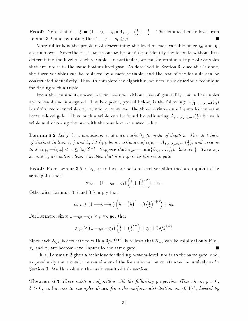
Proof: Note that � � � = (1 � �0 � �1)(Af jxj 1(12) � 1
2). The lemma then follows from
Lemma 3.2, and by noting that 1 � �0 � �1 � �.More di�cult is the problem of determining the level of each variable since �0 and �1
are unknown. Nevertheless, it turns out to be possible to identify the formula without �rst
determining the level of each variable. In particular, we can determine a triple of variables
that are inputs to the same bottom-level gate. As described in Section 3, once this is done,
the three variables can be replaced by a meta-variable, and the rest of the formula can be
constructed recursively. Thus, to complete the algorithm, we need only describe a technique
for �nding such a triple.
From the comments above, we can assume without loss of generality that all variables
are relevant and unnegated. The key point, proved below, is the following: ~Af jxi;xj;xk 1(12)
is minimized over triples xi, xj and xk whenever the three variables are inputs to the same
bottom-level gate. Thus, such a triple can be found by estimating ~Af jxi;xj;xk 1(12) for each
triple and choosing the one with the smallest estimated value.
Lemma 6.2 Let f be a monotone, read-once majority formula of depth h. For all triples
of distinct indices i, j and k, let �̂ijk be an estimate of �ijk = ~Af jxi;xj;xk 1(12), and assume
that j�ijk � �̂ijkj < � � 3�=2h+4. Suppose that �̂qrs = minf�̂ijk : i; j; k distinct g. Then xq,
xr and xs are bottom-level variables that are inputs to the same gate.
Proof: From Lemma 3.5, if xi, xj and xk are bottom-level variables that are inputs to the
same gate, then
�ijk = (1 � �0 � �1)�12+�12
�h�+ �0:
Otherwise, Lemmas 3.5 and 3.6 imply that
�ijk � (1� �0 � �1)�12 +
�12
�h+ 3
�12
�h+3�+ �0:
Furthermore, since 1� �0 � �1 � � we get that
�ijk � (1� �0 � �1)�12+�12
�h�+ �0 + 3�=2h+3:
Since each �̂ijk is accurate to within 3�=2h+4, it follows that �̂qrs can be minimal only if xq,
xr and xs are bottom-level inputs to the same gate.
Thus, Lemma 6.2 gives a technique for �nding bottom-level inputs to the same gate, and,
as previously mentioned, the remainder of the formula can be constructed recursively as in
Section 3. We thus obtain the main result of this section:
Theorem 6.3 There exists an algorithm with the following properties: Given h, n, � > 0,
� > 0, and access to examples drawn from the uniform distribution on f0; 1gn, labeled by
21

a read-once majority formula f of depth at most h on n variables, and misclassi�ed with
probabilities �0 and �1 (as described above) for �0+�1 � 1��, the algorithm exactly identi�es
f with probability at least 1� �. The algorithm's sample complexity is O((4h=�2) � log(n=�)),and its time complexity is O((4h=�2) � (n+ r3) � log(n=�)), where r is the number of relevant
variables appearing in the target formula.
Finally, we comment that our algorithms can be extended to handle a modest amount
of malicious noise. In this model, �rst considered by Kearns and Li [14], an adversary is
allowed to corrupt each example in any manner he chooses (both the labels and the variable
settings) with probability �. We can show that the algorithm described in Sections 3 for
majority formulas can handle malicious error rates as large as �(2�h) where h is the height
of the target formula. Thus, for logarithmic-depth formulas, we can handle malicious error
rates up to an inverse polynomial in the number of relevant variables. Similar results also
hold for nand formulas.
The extension of the algorithm to handle malicious noise is straightforward. The algo-
rithm of Section 3 depends only on accurate estimates of the ampli�cation of f when some
of f 's inputs are hard-wired. For instance, in the �rst phase of the algorithm, we need to
estimate, for each input xi, the ampli�cation � = Af jxi 1(12). This quantity is really just
the conditional probability
Pr[f = 1 j xi = 1] =Pr[f = 1 ^ xi = 1]
Pr[xi = 1]= 2 �Pr[f = 1 ^ xi = 1]
where the probabilities are computed with respect to the uniform distribution. Thus, we can
compute an estimate of � using an estimate for � = Pr[f = 1^xi = 1]. Note that malicious
noise can a�ect this probability � by at most an additive factor of �. That is, the chance
that f = 1 and xi = 1 (in the presence of malicious noise) is at least ��� and at most �+�.
Thus, using Hoe�ding's inequality (Lemma 3.9), an estimate of � that is accurate to
within �+� can be obtained from a sample of size polynomial in 1=� (with high probability).
Such an estimate for � yields an estimate for � that is accurate to within 2(� + � ).
A similar argument can be made for computing the estimates required in the second phase
of the algorithm. Since Theorems 3.3 and 3.7 show that the required estimates need only be
accurate to within 3=2h+4, it follows that a malicious error rate of, say, 1=16 this amount can
be tolerated without increasing the algorithm's complexity by more than constant factors.
7 Learning unbounded-depth formulas
In this �nal section, we describe extensions of our algorithms to learn formulas of unbounded
depth in Valiant's PAC model with respect to speci�c distributions. As in the last section,
22

we focus only on majority formulas, omitting the similar application of these techniques to
nand formulas.2
For formulas of unbounded depth, exact identi�cation from the uniform distribution
in polynomial time is too much to ask: For purely information-theoretic reasons, at least
(2h) examples must be drawn from the uniform distribution to exactly identify a majority
formula of depth h. This can be proved by showing (say, by induction on h) that if xi occurs
at level h of formula f , then 2�h is the probability that an instance is chosen for which the
output of f depends on xi (i.e., for which f 's output changes if xi is ipped). Thus, (2h)
random examples are needed simply to determine, for example, whether xi occurs negated
or unnegated.
Therefore, to handle arbitrarily deep formulas, we must relax our requirement of exact
identi�cation. Instead, we adopt Valiant's criterion of obtaining a good approximation of
the target concept (with high probability). As before, our algorithms do not work for all
distributions, just the �xed-point distribution. We describe an algorithm that, given �; � > 0
and access to random examples of the target majority formula drawn from the uniform
distribution, outputs with probability 1 � � an �-good hypothesis, that is, one that agrees
with the target formula on a randomly chosen instance from the uniform distribution with
probability at least 1 � �. Furthermore, the running time is polynomial in 1=�, 1=� and the
number of variables n.
We begin by brie y discussing the main ideas of the algorithm. First, as noted above,
variables that occur deep in the formula are unimportant in the sense that their values are
unlikely to in uence the formula's output on a randomly chosen instance. Intuitively, we
would like to take advantage of this fact by somehow treating such variables as irrelevant.
However, they cannot be simply deleted from the formula without leaving \holes" that must
in some way be handled.
We therefore introduce the notion of a partially visible function. This is a function on
a set of visible variables whose values can be observed by the learner, and a set of hidden
variables that are not observable. With respect to a distribution on the set of assignments
to the hidden variables, we say that two partially visible Boolean functions are equivalent if,
for all assignments to the visible variables, the probabilities are the same that each function
evaluates to 1 (where the probabilities are taken over random assignments to the hidden
variables). In other words, the behaviors of the two functions are indistinguishable with
respect to the visible variables.
Thus, we handle all deep variables by regarding them as hidden variables, and the target
2Alternatively, the algorithm recently described by Schapire [21] could be used to PAC-learn unbounded-
depth nand formulas. His algorithm is more general but less e�cient than the approach described in this
section.
23
formula as one that is partially visible. In particular, insigni�cant variables|those that
occur below level h = dlog(n=2�)e|are considered hidden and their actual values ignored.
We call the partially visible formula obtained from the target formula f in this manner the
truncated target.
Our algorithm works by exactly identifying the truncated target, that is, by constructing
a partially visible formula f 0 that is equivalent to it (in the sense described above, with
respect to the uniform distribution). It will be shown that f and f 0 agree on a randomly
chosen instance with probability at least 1 � �, and therefore f 0 is an �-good hypothesis
satisfying the PAC criterion.
It remains then only to show how f 0 can be constructed. First, observe that by Lemma 3.2
all signi�cant variables occurring in f can be detected (and their signs and levels determined)
in polynomial time. Moreover, by arguments similar to those given in Section 3, it can be
shown that if some triple of signi�cant variables meet at a gate, then the level of that gate
can be detected from the ampli�cation function by hard-wiring the three variables to 1. We
call this information (the level and sign of each signi�cant variable, and the level at which
each triple of signi�cant variables meet, if at all) the formula's schedule. It turns out that the
schedule alone is su�cient to fully re-construct the partially visible formula f 0, as is shown
below.
These then are the main ideas of the algorithm. What follows is a more detailed exposi-
tion.
A partially visible function f(x : y) is a Boolean function f on a set of visible variables x =
x1 � � �xr, and a set of hidden variables y = y1 � � � ys. Two partially visible functions f(x : y)
and g(x : z) on the same set of visible variables are equivalent with respect to distributions
D and E on the domains of y and z if, for all x, Pr[f(x : Y ) = 1] = Pr[g(x : Z) = 1], where
Y and Z are random variables representing a random assignment to y and z according to D
and E. In the discussion that follows, we will only be interested in uniform distributions.
As described above, our algorithm regards variables that occur deep in the target formula
as hidden variables. The next two lemmas show that two partially visible read-once majority
formulas that are identical, except for some deep hidden variables, are very likely to produce
the same output on randomly chosen inputs.
Lemma 7.1 Let f be a read-once majority formula on n variables. Let t be the level of xn
in f . Let X1; . . . ;Xn�1, Y and Z be independent Bernoulli variables, each 1 with probability
1=2. Then Pr[f(X1; . . . ;Xn�1; Y ) 6= f(X1; . . . ;Xn�1; Z)] = 2�t�1.
Proof: By induction on t. If t = 0, then f is the function xn and since Pr[Y 6= Z] =
1=2, the lemma holds. If t > 0, then let f = maj(f1; f2; f3), and suppose that f1 is the
subformula in which xn occurs. Since xn does not also occur in f2 or f3, we will regard
24
these as functions only on the remaining n � 1 variables. It is not hard to see then that
f(X1; . . . ;Xn�1; Y ) 6= f(X1; . . . ;Xn�1; Z) if and only if f2(X1; . . . ;Xn�1) 6= f3(X1; . . . ;Xn�1)
and f1(X1; . . . ;Xn�1; Y ) 6= f1(X1; . . . ;Xn�1; Z). Since f2 and f3 each output 1 independently
with probability 1=2, we have
Pr[f2(X1; . . . ;Xn�1) 6= f3(X1; . . . ;Xn�1)] = 1=2:
Also, by inductive hypothesis,
Pr[f1(X1; . . . ;Xn�1; Y ) 6= f1(X1; . . . ;Xn�1; Z)] = 2�t:
The lemma then follows by independence.
Lemma 7.2 Let f be a read-once majority formula on n variables. Let ti be the level of vari-
able xi in f . Let X1; . . . ;Xn;X01; . . . ;X
0r, r � n, be independent Bernoulli variables, each 1
with probability 1=2. Then Pr[f(X1; . . . ;Xn) 6= f(X 01; . . . ;X0r;Xr+1; . . . ;Xn)] � Pr
i=1 2�ti�1.
Proof: By induction on r. If r = 0, then the lemma holds trivially. For r > 0, we have
Pr[f(X1; . . . ;Xn) 6= f(X 01; . . . ;X0r;Xr+1; . . . ;Xn)]
� Pr[f(X1; . . . ;Xn) 6= f(X 01; . . . ;X0r�1;Xr; . . . ;Xn)]
+Pr[f(X 01; . . . ;X0r�1;Xr; . . . ;Xn) 6= f(X 01; . . . ;X
0r;Xr+1; . . . ;Xn)]
�r�1Xi=1
2�ti�1 + 2�tr�1
where the last inequality follows from our inductive hypothesis and the preceding lemma.
As proved below, Lemma 7.2 implies that any partially visible formula is an �-good
hypothesis if it is equivalent to the truncated target, the partially visible formula obtained
from the target formula by regarding all variables at or below level h = dlog(n=2�)e as hiddenvariables. Given an assignment to the visible variables, such a hypothesis is evaluated in the
obvious manner by choosing a random assignment to the hidden variables and computing
the output of the formula on the combined assignments to the hidden and visible variables.
(Thus, the hypothesis is likely to be randomized.)
Lemma 7.3 Let � > 0, and let f be a read-once majority formula on n variables. Let
x = x1 � � �xr be the variables occurring above level h = dlog(n=2�)e, and let y = y1 � � � yn�rbe the remaining variables. Let g(x : z) be any partially visible formula equivalent to the
partially visible formula f(x : y). Then Pr[f(X : Y ) 6= g(X : Z)] � �, where X, Y and Z
are random variables representing the uniformly random choice of assignments to x, y and
z. That is, g(x : z) is an �-good hypothesis for f .
25
Proof: Let Y 0 be a random variable representing a random assignment to y, chosen inde-
pendently of Y . Since f(x : y) is equivalent to g(x : z), we have
Pr[f(X : Y ) 6= g(X : Z)] = Pr[f(X : Y ) 6= f(X : Y 0)]:
By Lemma 7.2, the right hand side of this equation is bounded by �, since each of the
n� r � n variables yi occurs at or below level h in f .
For � > 0 and target formula f , we will henceforth say that variables occurring above
level h = dlog(n=2�)e are signi�cant. Note that Theorem 3.3 implies that the signi�cance,
sign and level of any variable xj can be determined by hard-wiring that variable to 1, as
usual. More speci�cally, if �̂ is an estimate of � = Af jxj 1(12) for which j�̂ � �j < � �
�12
�h+2
then xj is signi�cant if and only if����̂ � 1
2
��� > �12
�h+1+ � , and, if it is signi�cant, then its sign
and level can be determined as in Theorem 3.3.
Similar to Theorem 3.7, we can show that, for any triple of signi�cant variables, we can
determine the level of the gate at which the triple meets, if at all. More precisely, if xi, xj and
xk are three unnegated variables occurring at levels t1, t2 and t3, and if �̂ is an estimate of
� = Af jxi;xj;xk 1(12) for which j�̂� �j < � � 2�3h, then it follows from Lemmas 3.5 and 3.6
that xi, xj and xk meet at a level-d gate if and only if����12 +
�12
�t1+1+�12
�t2+1+�12
�t3+1 � �12
�t1+t2+t3�2d�1 � �̂���� < �:
As mentioned above, we call the sum total of this information|the signi�cance of each
variable, the level and sign of each signi�cant variable, and the level of the gate at which each
triple of signi�cant variables meet, if at all|the formula's schedule. It remains then only
to show how an �-good hypothesis can be constructed from the schedule. Speci�cally, we
show how to construct a partially visible formula that is equivalent to the truncated target
f(x : y). (Here, x is the vector of visible (i.e., signi�cant) variables, and y is the vector of
hidden (insigni�cant) variables.)
Suppose �rst that no three visible variables meet in f . Such a formula is said to be
unstructured. Although strictly speaking f cannot be unstructured (by our choice of h), this
special case turns out nevertheless to be important in handling the more general case since
subformulas of f may be unstructured.
Lemma 7.4 below shows that an unstructured formula f(x : y) is equivalent to any other
unstructured partially visible formula whenever each visible variable occurs at the same level
with the same sign in both formulas. Thus, unstructured formulas are not changed when
visible variables are moved around within the same level. This fact makes the identi�cation
of unstructured formulas from their schedules quite easy.
For any partially visible read-once majority formula f(x : y), let pf (x) = Pr[f(x : Y ) = 1]
where Y represents a random assignment to y.
26

Lemma 7.4 Let f(x : y) and g(x : z) be unstructured read-once majority formulas on s
visible variables. Suppose that each visible variable xj is relevant and occurs at the same
level tj with the same sign in both formulas. Then the two partially visible formulas are
equivalent.
Proof: It su�ces to prove the lemma when no visible variable is negated since negated
variables can simply be replaced by unnegated meta-variables.
To prove the lemma, we show that
pf (x) =12+
sXi=1
2�ti(xi � 12): (1)
Since this statement applies to any unstructured formula, it follows immediately that pf (x) =
pg(x) and the two partially visible formulas are equivalent.
We prove Equation (1) by induction on the height h of f . If h = 0, then f consists of
a single visible or hidden variable. If f is the formula xj, where xj is some visible variable,
then pf (x) = xj, satisfying (1). If f is the formula yj, where yj is a hidden variable, then
pf (x) =12 , also satisfying (1).
If h > 0, then let f = maj(f1; f2; f3) where f1, f2 and f3 are partially visible subformulas.
Since f is unstructured, one of these (say f3) contains no visible variables, and thus pf3(x) =12 . Suppose without loss of generality that x1; . . . ; xr are the visible variables relevant to f1.
Then, by inductive hypothesis,
pf1(x) =12+
rXi=1
2�ti+1(xi � 12)
and
pf2(x) =12 +
sXi=r+1
2�ti+1(xi � 12):
Applying Lemma 3.1, it is easily veri�ed that Equation (1) is satis�ed, completing the
induction.
Thus, if f(x : y) is unstructured, then an equivalent unstructured formula can be con-
structed from f 's schedule. For instance, here is an e�cient algorithm: Let t be the depth
of the deepest visible variable in f . Break the set of all level-t variables into pairs. Replace
each such pair xi; xj by a level-(t� 1) visible meta-variable w � maj(xi; xj; y), where y is
a new hidden variable. If an odd level-t variable xi remains, replace it with a level-(t� 1)
visible meta-variable w � maj(xi; y; y0), where y and y0 are new hidden variables. Repeat
for levels t� 1; t � 2; . . . ; 1. It is not hard to show that this algorithm results in a formula
that is unstructured, and that is consistent with f 's schedule (and so is equivalent).
With these tools in hand for dealing with unstructured formulas, we are now ready
to describe an algorithm for handling the general case, i.e., for reconstructing any (not
necessarily unstructured) formula from its schedule.
27
Let f(x : y) be the truncated target. If f is unstructured, then the previous algorithm
applies. Otherwise, we can �nd from the schedule three visible variables xi, xj and xk that
meet at some maximum-depth gate � of f ; that is, they meet at a level-d gate, and no triple
of visible variables meet at any gate of depth exceeding d. Then the subformula g subsumed
by � computes the majority of three subformulas g1, g2 and g3, each containing one of xi, xj
and xk (say, in that order). Let x` be some other visible variable. Then it is easily veri�ed
that x` is relevant to g1 if and only if x`, xj and xk meet at a level-d gate (namely, �). Thus,
all of the visible variables relevant to g1 (and likewise for g2 and g3) can be determined from
the schedule. Moreover, note that each of these subformulas is unstructured since � is of
maximum depth. Thus, each subformula can be identi�ed using the previous algorithm for
unstructured formulas, and therefore, the entire subformula subsumed by (and including) �
can be identi�ed.
The rest of the formula can be identi�ed recursively: we replace subformula g by a new
meta-variable w, and update the schedule appropriately.
This completes the description of the algorithm. We thus have:
Theorem 7.5 There exists an algorithm with the following properties: Given n, � > 0,
and access to examples drawn from the uniform distribution on f0; 1gn and labeled by any
read-once majority formula f on n variables, the algorithm outputs an �-good hypothesis for
f with probability at least 1 � �. The algorithm's sample complexity is O((n=�)6 � log(n=�)),and its time complexity is O((n9=�6) � log(n=�)).
Proof: As before, let h = dlog(n=2�)e. To implement the procedure outlined above, we
must be able to compute from a random sample: (1) each variable's signi�cance, (2) each
signi�cant variable's sign and level, and (3) the level of the gate (if any) at which each triple
of signi�cant variables meet. As noted above, to compute (1) and (2), we need to �nd, for
each variable xi, an estimate �̂ of � = Af jxi 1(12) for which j�� �̂j <
�12
�h+2. Hoe�ding's
inequality (Lemma 3.9) implies that such estimates can be derived, with high probability,
from a sample of size O(22h log(n=�)). We also noted above that we can compute (3) given,
for each triple of signi�cant variables xi; xj; xk, an estimate �̂ of � = Af jxi;xj ;xk 1(12) for
which j�̂� �j < 2�3h. Again applying Hoe�ding's inequality, we see that such estimates
can be computed (with high probability) for all triples of variables from a sample of size
O(26h log(n=�)). This proves the stated sample size.
The running time of the procedure is dominated by the computation from the sample of
the O(n3) estimates described above.
28

8 Summary
In this paper, we have described a general technique for inferring the structure of read-once
formulas over various bases. We have shown how this technique can be applied to achieve
exact identi�cation when the formula is of logarithmic depth, even in the presence of noise.
We have also described how to use this technique to infer good approximations of formulas
with unbounded depth.
9 Acknowledgements
We are very grateful to Ron Rivest for his comments on this material, and for a careful
reading he made of an earlier draft. We also thank Avrim Blum for suggesting the notion
of a universal identi�cation sequence. Finally, we thank the anonymous referees for their
comments.
References
[1] Dana Angluin, Lisa Hellerstein, and Marek Karpinski. Learning read-once formulas
with queries. Technical Report UCB/CSD 89/528, University of California Berkeley,
Computer Science Division, August 1989. To appear, Journal of the Association for
Computing Machinery.
[2] Dana Angluin and Philip Laird. Learning from noisy examples. Machine Learning,
2(4):343{370, 1988.
[3] Gyora M. Benedek and Alon Itai. Learnability by �xed distributions. In Proceedings of
the 1988 Workshop on Computational Learning Theory, pages 80{90, August 1988.
[4] Ravi B. Boppana. Ampli�cation of probabilistic Boolean formulas. In 26th Annual
Symposium on Foundations of Computer Science, pages 20{29, October 1985.
[5] Ravi Babu Boppana. Lower Bounds for Monotone Circuits and Formulas. PhD thesis,
Massachusetts Institute of Technology, 1986.
[6] N. Bshouty, T. Hancock, L. Hellerstein, and M. Karpinski. Read-once formulas, justi-
fying assignments, and generic transformations. Unpublished Manuscript, 1991.
[7] Merrick Furst, Je�rey Jackson, and Sean Smith. Learning AC0 functions sampled
under mutually independent distributions. Technical Report CMU-CS-90-183, Carnegie
Mellon University, School of Computer Science, October 1990.
29

[8] Sally A. Goldman and Michael J. Kearns. On the complexity of teaching. In Proceedings
of the Fourth Annual Workshop on Computational Learning Theory, pages 303{314,
August 1991.
[9] Thomas Hancock and Lisa Hellerstein. Learning read-once formulas over �elds and ex-
tended bases. In Proceedings of the Fourth Annual Workshop on Computational Learning
Theory, pages 326{336, August 1991.
[10] Thomas Hancock and Yishay Mansour. Learning monotone k� DNF formulas on prod-
uct distributions. In Proceedings of the Fourth Annual Workshop on Computational
Learning Theory, pages 179{183, August 1991.
[11] Lisa Hellerstein. On Characterizing and Learning Some Classes of Read-Once Formulas.
PhD thesis, University of California at Berkeley, 1989.
[12] Wassily Hoe�ding. Probability inequalities for sums of bounded random variables. Jour-
nal of the American Statistical Association, 58(301):13{30, March 1963.
[13] Michael Kearns. The Computational Complexity of Machine Learning. MIT Press, 1990.
[14] Michael Kearns and Ming Li. Learning in the presence of malicious errors. In Proceedings
of the Twentieth Annual ACM Symposium on Theory of Computing, pages 267{280, May
1988.
[15] Michael Kearns, Ming Li, Leonard Pitt, and Leslie Valiant. On the learnability of
Boolean formulae. In Proceedings of the Nineteenth Annual ACM Symposium on Theory
of Computing, pages 285{295, May 1987.
[16] Michael Kearns and Leslie G. Valiant. Cryptographic limitations on learning Boolean
formulae and �nite automata. In Proceedings of the Twenty First Annual ACM Sym-
posium on Theory of Computing, pages 433{444, May 1989.
[17] Nathan Linial, Yishay Mansour, and Noam Nisan. Constant depth circuits, Fourier
transform, and learnability. In 30th Annual Symposium on Foundations of Computer
Science, pages 574{579, October 1989.
[18] Giulia Pagallo and David Haussler. A greedy method for learning �DNF functions under
the uniform distribution. Technical Report UCSC-CRL-89-12, University of California
Santa Cruz, Computer Research Laboratory, June 1989.
[19] Leonard Pitt and Manfred K. Warmuth. Prediction-preserving reducibility. Journal of
Computer and System Sciences, 41(3):430{467, December 1990.
30

[20] Robert E. Schapire. The strength of weak learnability. Machine Learning, 5(2):197{227,
1990.
[21] Robert E. Schapire. Learning probabilistic read-once formulas on product distributions.
In Proceedings of the Fourth Annual Workshop on Computational Learning Theory,
pages 184{198, August 1991.
[22] Ayumi Shinohara and Satoru Miyano. Teachability in computational learning. New
Generation Computing, 8:337{247, 1991.
[23] Robert H. Sloan. Types of noise in data for concept learning. In Proceedings of the 1988
Workshop on Computational Learning Theory, pages 91{96, August 1988.
[24] Leslie G. Valiant. A theory of the learnable. Communications of the ACM, 27(11):1134{
1142, November 1984.
[25] Karsten Verbeurgt. Learning DNF under the uniform distribution in quasi-polynomial
time. In Proceedings of the Third Annual Workshop on Computational Learning Theory,
pages 314{326, August 1990.
31


