
NBER WORKING PAPER SERIES
EXPLAINING THE FAVORITE-LONGSHOT BIAS:IS IT RISK-LOVE OR MISPERCEPTIONS?
Erik SnowbergJustin Wolfers
Working Paper 15923http://www.nber.org/papers/w15923
NATIONAL BUREAU OF ECONOMIC RESEARCH1050 Massachusetts Avenue
Cambridge, MA 02138April 2010
We thank David Siegel of Equibase for supplying the data, and Scott Hereld and Ravi Pillai for theirvaluable assistance in managing the data. Jon Bendor, Bruno Jullien, Steven Levitt, Kevin Murphy,Marco Ottaviani, Bernard Salanie, Peter Norman Sørenson, Betsey Stevenson, Matthew White, WilliamZiemba and an anonymous referee provided useful feedback, as did seminar audiences at CarnegieMellon, Chicago GSB, Haas School of Business, Harvard Business School, University of Lausanne,Kellogg (MEDS), University of Maryland, University of Michigan and Wharton. Snowberg gratefullyacknowledges the SIEPR Dissertation Fellowship through a grant to the Stanford Institute for EconomicPolicy Research. Wolfers gratefully acknowledges a Hirtle, Callaghan & Co.–Arthur D. MiltenbergerResearch Fellowship, and the support of the Zull/Lurie Real Estate Center, the Mack Center for TechnologicalInnovation, and Microsoft Research. The views expressed herein are those of the authors and do notnecessarily reflect the views of the National Bureau of Economic Research.
© 2010 by Erik Snowberg and Justin Wolfers. All rights reserved. Short sections of text, not to exceedtwo paragraphs, may be quoted without explicit permission provided that full credit, including © notice,is given to the source.
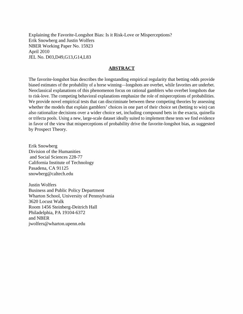
Explaining the Favorite-Longshot Bias: Is it Risk-Love or Misperceptions?Erik Snowberg and Justin WolfersNBER Working Paper No. 15923April 2010JEL No. D03,D49,G13,G14,L83
ABSTRACT
The favorite-longshot bias describes the longstanding empirical regularity that betting odds providebiased estimates of the probability of a horse winning—longshots are overbet, while favorites are underbet.Neoclassical explanations of this phenomenon focus on rational gamblers who overbet longshots dueto risk-love. The competing behavioral explanations emphasize the role of misperceptions of probabilities.We provide novel empirical tests that can discriminate between these competing theories by assessingwhether the models that explain gamblers’ choices in one part of their choice set (betting to win) canalso rationalize decisions over a wider choice set, including compound bets in the exacta, quinellaor trifecta pools. Using a new, large-scale dataset ideally suited to implement these tests we find evidencein favor of the view that misperceptions of probability drive the favorite-longshot bias, as suggestedby Prospect Theory.
Erik SnowbergDivision of the Humanities and Social Sciences 228-77California Institute of TechnologyPasadena, CA 91125 [email protected]
Justin WolfersBusiness and Public Policy DepartmentWharton School, University of Pennsylvania3620 Locust WalkRoom 1456 Steinberg-Deitrich HallPhiladelphia, PA 19104-6372and [email protected]

1 Introduction
The racetrack provides a natural laboratory for economists interested in understanding decision-
making under uncertainty. The most discussed empirical regularity in racetrack gambling markets
is the favorite-longshot bias: equilibrium market prices (betting odds) provide biased estimates
of the probability of a horse winning. Specifically, bettors value longshots more than expected
given how rarely they win, and they value favorites too little given how often they win. Figure
1 illustrates, showing that the rate of return to betting on horses with odds of 100/1 or greater is
about −61%, betting randomly yields average returns of −23%, while betting the favorite in every
race yields losses of only 5.5%.
Figure 1: The rate of return on win bets declines as risk increases.
Even Break
−20
−40
−60
−80
Rat
e of
Ret
urn
per
Doll
ar B
et (
%)
1/3 1/2 Evens 2/1 5/1 10/1 20/1 50/1 100/1 200/1Odds (Log Scale)
Raw data: Aggregated into percentiles
All Races
Subsample: Exotic betting data available
Subsample: Last Race of the Day
Sample: US Horse Races, 1992−2001
The Favorite−Longshot Bias
Notes: Sample includes 5,610,580 horse race starts in the United States from 1992–2001.Lines reflect Lowess smoothing (bandwidth=0.4).
Since the favorite-longshot bias was first noted by Griffith in 1949, it has been found in race-
track betting data around the world, with very few exceptions. The literature documenting this bias
1

is voluminous, and covers both bookmaker- and pari-mutuel markets.1
Two broad sets of theories have been proposed to explain the favorite-longshot bias. First,
neoclassical theory suggests that the prices bettors are willing to pay for various gambles can
be used to recover their utility function. While betting at any odds is actuarially unfair, this is
particularly acute for longshots—which are also the riskiest investments. Thus, the neoclassical
approach can reconcile both gambling and the longshot bias only by positing (at least locally)
risk-loving utility functions, as in Friedman and Savage (1948).
Alternatively, behavioral theories suggest that cognitive errors and misperceptions of probabil-
ities play a role in market mis-pricing. These theories incorporate laboratory studies by cognitive
psychologists that show people are systematically poor at discerning between small and tiny prob-
abilities, and hence price both similarly. Further, people exhibit a strong preference for certainty
over extremely likely outcomes, leading highly probable gambles to be under-priced. These results
form an important foundation of Prospect Theory (Kahneman and Tversky, 1979).
Our aim in this paper is to test whether the risk-love class of models or the misperceptions class
of models simultaneously fits data from multiple betting pools. While there exist many specific
models of the favorite-longshot bias, we show in Section 3 that each yields implications for the
pricing of gambles equivalent to stark models of either a risk-loving representative agent, or a
representative agent who bases her decisions on biased perceptions of true probabilities. That is,
the favorite-longshot bias can be fully rationalized by a standard rational-expectations expected-
utility model, or by appealing to an expected wealth maximizing agent who overweights small
probabilities and underweights large probabilities.2 Thus, without parametric assumptions, which
we are unwilling to make, the two theories are observationally equivalent in win bet data.
We combine new data with a novel econometric identification strategy to discriminate between
1Thaler and Ziemba (1988), Sauer (1998) and Snowberg and Wolfers (2007) survey the literature. The exceptionsare Busche and Hall (1988), which finds that the favorite-longshot bias is not evident in data on 2,653 Hong Kongraces, and Busche (1994), which confirms this finding in an additional 2,690 races in Hong Kong, and 1,738 races inJapan.
2Or adopting a behavioral versus neoclassical distinction, we follow Gabriel and Marsden (1990) in asking: “arewe observing an inefficient market or simply one in which the tastes and preferences of the market participations leadto the observed results?”
2

these two classes of theories. Our data include all 6.4 million horse race starts in the United
States from 1992 to 2001. These data are an order of magnitude larger than any dataset previously
examined, and allow us to be extremely precise in establishing the relevant stylized facts.
Our econometric innovation is to distinguish between these theories by deriving testable pre-
dictions about the pricing of compound lotteries (also called exotic bets at the racetrack). For
example, an exacta is a bet on both which horse will come first and which will come second. Es-
sentially, we ask whether the preferences and perceptions that rationalize the favorite-longshot bias
(in win bet data) can also explain the pricing of exactas, quinellas—a bet on two horses to come
first and second in either order—and trifectas—a bet on which horse will come in first, which
second and which third. By expanding the choice set under consideration (to correspond with the
bettor’s actual choice set!), we use each theory to derive unique testable predictions. We find that
the misperceptions class more accurately predicts the prices of exotic bets, and also their relative
prices.
To demonstrate the application of this idea to our data, note that betting on horses with odds
between 4/1 and 9/1 has an approximately constant rate of return (at −18%, see Figure 1). Thus,
the misperceptions class infers bettors are equally well calibrated over this range, and hence betting
on combinations of outcomes among such horses will yield similar rates of return. That is, betting
on an exacta with a 4/1 horse to win and a 9/1 horse to come second will yield similar expected
returns to betting on the exacta with the reverse ordering (although the odds of the two exactas will
differ). In contrast, under the risk-love model, bettors are willing to pay a larger risk penalty for
the riskier bet—such as the exacta in which the 9/1 horse wins, and the 4/1 horse runs second—
decreasing its rate of return relative to the reverse ordering.
Our research question is most similar to Jullien and Salanie (2000) and Gandhi (2007) who
attempt to differentiate between preference- and perception-based explanations of the favorite-
longshot bias using only data on the price of win bets. The results of the former study favor
perception-based explanations and the results of the latter favor preference-based explanations.
Rosett (1965) conducts a related analysis in that he considers both win bets and combinations of
3

win bets as present in the bettors’ choice set. Ali (1979), Asch and Quandt (1987) and Dolbear
(1993) test the efficiency of compound lottery markets. We believe that we are the first to use com-
pound lottery prices to distinguish between competing theories of possible market (in)efficiency.
Of course the idea is much older: Friedman and Savage (1948) notes that a hallmark of expected
utility theory is “that the reaction of persons to complicated gambles can be inferred from their
reaction to simple gambles.”
2 Stylized Facts
Our data contains all 6,403,712 horse starts run in the United States between 1992 and 2001. These
are official jockey club data; the most precise available. Data of this nature are extremely expen-
sive, which presumably explains why previous studies have used substantially smaller samples.
The appendix provides more detail about the data.
We summarize our data in Figure 1. We calculate the rate of return to betting on every horse at
each odds, and use Lowess smoothing to take advantage of information from horses with similar
odds. Data are graphed on a log-odds scale so as to better show their relevant range. The vastly
better returns to betting on favorites rather than longshots is the favorite-longshot bias. Figure
1 also shows the same pattern for the 206,808 races (with 1,485,112 horse starts) for which the
jockey club recorded payoffs to exacta, quinella or trifecta bets. Given that much of our analysis
will focus on this smaller sample, it is reassuring to see a similar pattern of returns.
Figure 2 shows the same rate of return calculations for several other datasets. We present new
data from 2,725,000 starts in Australia from the South Coast Database, and 380,000 starts in Great
Britain from flatstats.co.uk. The favorite-longshot bias appears equally evident in these countries,
despite the fact that odds are determined by pari-mutuel markets in the United States, bookmakers
in the United Kingdom, and bookmakers competing with a state-run pari-mutuel market in Aus-
tralia. Figure 2 also includes historical estimates of the favorite-longshot bias, showing it has been
stable since first noted in Griffith (1949).
4
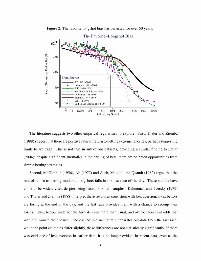
Figure 2: The favorite longshot bias has persisted for over 50 years.
Even Break
−20
−40
−60
−80
Rat
e of
Ret
urn
per
Doll
ar B
et (
%)
1/3 1/2 Evens 2/1 5/1 10/1 20/1 50/1 100/1 200/1Odds (Log Scale)
US: 1992−2001
Australia: 1991−2004
UK: 1994−2004
Griffith, Am. J. Psych 1949
Weitzman, JPE 1965
Harville, JASA 1973
Ali, JPE 1977
Jullien and Salanie, JPE 2000
Data Source
The Favorite−Longshot Bias
The literature suggests two other empirical regularities to explore. First, Thaler and Ziemba
(1988) suggest that there are positive rates of return to betting extreme favorites, perhaps suggesting
limits to arbitrage. This is not true in any of our datasets, providing a similar finding to Levitt
(2004): despite significant anomalies in the pricing of bets, there are no profit opportunities from
simple betting strategies.
Second, McGlothlin (1956), Ali (1977) and Asch, Malkiel, and Quandt (1982) argue that the
rate of return to betting moderate longshots falls in the last race of the day. These studies have
come to be widely cited despite being based on small samples. Kahneman and Tversky (1979)
and Thaler and Ziemba (1988) interpret these results as consistent with loss aversion: most bettors
are losing at the end of the day, and the last race provides them with a chance to recoup their
losses. Thus, bettors underbet the favorite even more than usual, and overbet horses at odds that
would eliminate their losses. The dashed line in Figure 1 separates out data from the last race;
while the point estimates differ slightly, these differences are not statistically significantly. If there
was evidence of loss aversion in earlier data, it is no longer evident in recent data, even as the
5

favorite-longshot bias has persisted.
In the next section we argue that these facts cannot separate risk-love from misperception-
based theories. We propose new tests based on the requirement that a theory developed to explain
equilibrium odds of horses winning should also be able to explain the equilibrium odds in the
exacta, quinella and trifecta markets separately, as well as the equilibrium odds in exacta and
quinella markets jointly.
3 Two Models of the Favorite-Longshot Bias
We start with two extremely stark models, each of which has the merit of simplicity. Both are
models where all agents have the same preferences and perceptions, but as we suggest below, can
be expanded to incorporate heterogeneity. Equilibrium price data cannot separately identify more
complex models from these representative agent models.
3.1 The Risk-Love Class
Following Weitzman (1965), we postulate expected utility maximizers with unbiased beliefs and
utility U(·): R→ R. In equilibrium, bettors must be indifferent between betting on the favorite
horse A with probability of winning pA and odds of OA/1, and betting on a longshot B with proba-
bility of winning pB and odds of OB/1:
pAU(OA) = pBU(OB) (normalizing utility to zero, if the bet is lost).3 (1)
The odds (OA, OB) and the probabilities (pA, pB) of horses winning, which we observe, identify
the representative bettor’s utility function up to a scaling factor.4 To fix the scale we normalize
utility to zero if the bet loses, and to one if the bettor chooses not to bet. Thus, if the bettor is
indifferent between accepting or rejecting a gamble offering odds of O/1 that wins with probability
3We also assume that, consistent with the literature, each bettor chooses to bet on only one horse in a race.4See Weitzman (1965), Ali (1977), Quandt (1986) and Jullien and Salanie (2000) for prior examples.
6

Figure 3: The win data is completely rationalized by both classes.U
tili
ty
W0 W0+20b W0+40b W0+60b W0+80b W0+100bWealth [Units: W0=Initial Wealth; b=Bet Size]
Utility Functionfully rationalizing Longshot bias
Risk Neutral Utility Function
Constant Absolute Risk AversionArrow−Pratt CARA=−.017 (risk love)
Assuming Unbiased Expectations
Risk−Loving Utility Function
.005
.01
.02
.05
.1
.2
.5
1
Per
ceiv
ed P
robab
ilit
y (
Log s
cale
)
.005 .01 .02 .05 .1 .2 .5 1Actual Probability (Log scale)
Probability Weightingfully rationalizing Longshot bias
Unbiased Expectations
Prelec weighting function:ln(pi)=−[−ln(prob)]^aa=.928
Assuming Risk−Neutrality
Probability Weighting Function
p, then U(O) =1p
. The left panel of Figure 3 performs precisely this analysis, backing out the
utility function required to explain all of the variation in Figure 1.
As can be seen from Figure 3, a risk-loving utility function is required to rationalize the bettor
accepting lower average returns on longshots, even as they are riskier bets. The figure also shows
that a CARA utility function fits the data reasonably well.
Several other theories of the favorite-longshot bias yield implications that are observation-
ally equivalent to this risk-loving representative agent model. Some of these theories are clearly
equivalent—such as that of Golec and Tamarkin (1998), which argues that bettors prefer skew
rather than risk—as they are theories about the shape of the utility function. It can easily be shown
that richer theories—such as that of Thaler and Ziemba (1988) where “bragging rights” accrue
from winning a bet at long odds, or that of Conlisk (1993) in which the mere purchase of a bet on
7

a longshot may confer some utility—are also equivalent.5
3.2 The Misperceptions Class
Alternatively, the misperceptions class postulates risk-neutral subjective expected utility maximiz-
ers, whose subjective beliefs are given by the probability weighting function π(p): [0,1]→ [0,1].
In equilibrium, there are no opportunities for subjectively-expected gain, so bettors must believe
that the subjective rates of return to betting on any pair of horses A and B are equal:
π(pA)(OA +1) = π(pB)(OB +1) = 1. (2)
Consequently, data on the odds (OA, OB) and the probabilities (pA, pB) of horses winning reveal
the misperceptions of the representative bettor.6
Note that the misperceptions class allows more flexibility in the way probabilities enter the
representative bettor’s value of a bet, but it is more restrictive than the risk-love class in terms of
how payoffs enter that function. More to the point, without restrictive parametric assumptions,
each class of models is just-identified, so each yields identical predictions for the pricing of win
bets.
The right panel of Figure 3 shows the probability weighting function π(p) implied by the data
in Figure 1. The low rates of return to betting longshots are rationalized by bettors who bet as
though horses with tiny probabilities of winning actually have moderate probabilities of winning.
The specific shape of the declining rates of return identifies the probability weighting function at
5Formally, these theories suggest agents maximize expected utility, where utility is the sum of the felicity ofwealth, y(·): R→ R, and the felicity of bragging rights or the thrill of winning, b(·): R→ R. Hence the expectedutility to a bettor with initial wealth w0 of a gamble at odds O that wins with probability p can be expressed as:E(U(O)) = p[y(w0 + O)+ b(O)] + [1− p]y(w0− 1). As before, bettors will accept lower returns on riskier wagers(betting on longshots) if U ′′ > 0. This is possible if either the felicity of wealth is sufficiently convex or braggingrights are increasing in the payoff at a sufficiently increasing rate. More to the point, revealed preference data do notallow us to separately identify effects operating through y(·), rather than b(·).
6While we term the divergence between π(p) and p misperceptions, in non-expected utility theories, π(p) canbe interpreted as a preference over types of gambles. Under either interpretation our approach is valid, in that wetest whether gambles are motivated by nonlinear functions of wealth or probability. In (2) we implicitly assume thatπ(1) = 1, although we allow limp→1 π(p)≤ 1.
8

each point.7 This function shares some of the features of the decision weights in Prospect Theory
(Kahneman and Tversky, 1979), and the figure shows that the one-parameter probability weighting
function in Prelec (1998) fits the data quite closely.
While we have presented a very sparse model, a number of richer theories have been proposed
that yield similar implications.8 For instance, Ottaviani and Sørenson (2009) show that initial infor-
mation asymmetries between bettors may lead to misperceptions of the true probabilities of horses
winning. Moreover, Henery (1985) and Williams and Paton (1997) argue that bettors discount a
constant proportion of the gambles in which they bet on a loser, possibly due to a self-serving bias
in which losers argue that conditions were atypical. Because longshot bets lose more often, this
discounting yields perceptions in which betting on a longshot seems more attractive.
3.3 Implications for Pricing Compound Lotteries
We now show how our two classes of models—while each just-identified based on data from win
bets—yield different implications for the prices of exotic bets. As such, our approach responds to
Sauer (1998, p.2026), which calls for research that provides “equilibrium pricing functions from
well-posed models of the wagering market.”
We discuss the pricing of exactas (picking the first two horses in order) in detail. Prices for these
bets are constructed from: the bettors’ utility function, indifference conditions as in (1) or (2), data
on the perceived likelihood of the pick for first, A, actually winning (pA or π(pA), depending on
the class), and conditional on A winning, the likelihood of the pick for second, B, coming second
(pB|A or π(pB|A)). A bettor will be indifferent between betting on an exacta on horses A then B in
that order, paying odds of EAB/1, and not betting (which yields no change in wealth, and hence a
7 There remains one minor issue: as Figure 1 shows, horses never win as often as suggested by their win oddsbecause of the track-take. Thus we follow the convention in the literature and adjust the odds-implied probabilitiesby a factor of one minus the track take for that specific race, so that they are on average unbiased; our results arequalitatively similar whether or not we make this adjustment.
8While the assumption of risk-neutrality may be too stark, as long as bettors gamble small proportions of theirwealth the relevant risk premia are second-order. For instance, assuming log utility, if the bettor is indifferent overbetting x% of their wealth on horse A or B, then: π(pA) log(w + wxOA)+ (1−π(pA)) log(w−wx) = π(pB) log(w +wxOB)+(1−π(pB)) log(w−wx), which under the standard approximation simplifies to: π(pA)(OA +1)≈ π(pB)(OB +1), as in (2).
9

utility of one), if:
Risk-Love Class
(Risk-lover, Unbiased expectations)
pA pB|AU(EAB) = 1
Noting p =1
U(O)from (1)
EAB = U -1(U(OA)U(OB|A))
(3)
Misperceptions Class
(Biased expectations, Risk-neutral)
π(pA)π(pB|A)(EAB +1) = 1
Noting π(p) =1
O+1from (2)
EAB = (OA +1)(OB|A +1)−1 (4)
Thus, under the misperceptions class, the odds of the exacta EAB are a simple function of the
odds of horse A winning, OA, and conditional on this, on the odds of B coming second, OB|A. The
preferences class is more demanding, requiring that we estimate the utility function. The utility
function is estimated from the pricing of win bets (in Figure 3), and can be inverted to compute
unbiased win probabilities from the betting odds.9
Our empirical tests simply determine which of (3) or (4) better fit the actual prices of exacta
bets. We apply an analogous approach to the pricing of quinella and trifecta bets: the intuition is
the same; the mathematical details are described in Appendix B.
Note that both (3) and (4) require OB|A, which is not directly observable. In Section 4 we
infer the conditional probability pB|A (and hence π(pB|A) and OB|A) from win odds by assuming
that bettors believe in conditional independence. That is, we apply the Harville (1973) formula:
π(pB|A) =π(pB)
1−π(pA); replacing π(p) with p in the risk-love class. This assumption is akin to
thinking about the race for second as a “race within the race” (Sauer, 1998). While relying on the
Harville formula is standard in the literature—see for instance Asch and Quandt (1987)—we show
that our results are robust to dropping this assumption and estimating this conditional probability,
pB|A, directly from the data.
9Our econometric method imposes continuity on the utility and probability weighting functions; the data mandatethat both be strictly increasing. Together this is sufficient to ensure that π(·) and U(·) are invertible. As in Figure 1,we do not have sufficient data to estimate the utility of winning bets at odds greater than 200/1. This prohibits us frompricing bets whose odds are greater than 200/1, which is most limiting for our analysis of trifecta bets.
10
3.4 Failure to Reduce Compound Lotteries
As in Prospect Theory, the frame the bettor adopts in trying to assess each gamble is a key issue,
particularly for misperceptions-based models. Specifically, (4) assumes that bettors first attempt
to assess the likelihood of horse A winning, π(pA), and then assess the likelihood of B coming
second given that A is the winner, π(pB|A). An alternative frame might suggest that bettors directly
assesses the likelihood of first-and-second combinations: π(pA pB|A).10
There is a direct analogy to the literature on the assessment of compound lotteries: does the bet-
tor separately assess the likelihood of winning an initial gamble (picking the winning horse) which
yields a subsequent gamble as its prize (picking the second-placed horse), or does she consider the
equivalent simple lottery (as in Samuelson (1952))? Consistent with (4), the accumulated experi-
mental evidence (Camerer and Ho, 1994) is more in line with subjects failing to reduce compound
lotteries into simple lotteries.11
Alternatively, we could choose not to defend either assumption, leaving it as a matter for em-
pirical testing. Interestingly, if gamblers adopt a frame consistent with the reduction of compound
lotteries into their equivalent simple lottery form, this yields a pricing rule for the misperceptions
class equivalent to that of the risk-love class.12 Thus, evidence consistent with what we are calling
the risk-love class accommodates either risk-love by unbiased bettors, or risk-neutral but biased
bettors, whose bias affects their perception of an appropriately reduced compound lottery. By
contrast, the competing misperceptions class implies the failure to reduce compound lotteries and
posits the specific form of this failure, shown in (4).
This discussion implies that results consistent with our risk-love class are also consistent with
a richer set of models emphasizing choices over simple gambles. These include models based on
the utility of gambling, information asymmetry or limits to arbitrage, such as Ali (1977), Shin
10Unless the probability weighting function is a power function (π(p) = pα ), these different frames yield differentimplications (Aczel, 1966).
11Additionally, note that (4) satisfies the compound independence axiom of Segal (1990).12To see this, note that identical data (from Figure 1) is used to construct the utility and decision weight functions
respectively, so each is constructed to rationalize the same set of choices over simple lotteries. This implies eachclass also yields the same set of choices over compound lotteries if preferences in both classes obey the reduction ofcompound lotteries into equivalent simple lotteries.
11

(1992), Hurley and McDonough (1995), Manski (2006). Any theory that prescribes a specific bias
in a market for a simple gamble (win betting) will yield similar implications in a related market for
compound gambles if gamblers assess their equivalent simple gamble form. By implication, reject-
ing the risk-love class substantially narrows the set of plausible theories of the favorite-longshot
bias.
4 Results from Exotic Bets
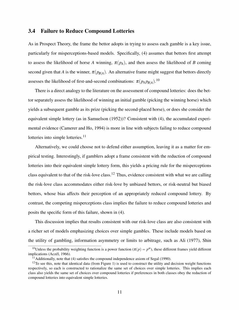
The first panel of Figure 4 shows the difference between the predictions for exactas of the risk-
love and misperceptions classes, expressed as a percent of the predictions. This demonstrates the
two classes of models yield qualitatively different predictions. Exotic bets have relatively low
probabilities of winning, so under the risk-love class a risk penalty results, yielding lower odds.
By contrast, the misperceptions model is based on the underlying simple lotteries, many of which
suffer smaller perception biases. The risk penalty becomes particularly important as odds get
longer; thus the difference in predictions grows along a line from the bottom right to the top left of
the first panel of Figure 4.
To focus on shorter-odds bets, in Table 1 we convert the predictions into the price of a con-
tingent contract that pays $1 if the chosen exacta wins: Price =1
Odds+1. We test the ability of
each economic model to predict this price by examining the mean absolute error of the predictions
of both models from the actual prices of exotic bets (column 1). We further investigate which of
the models produces predictions that are closer, observation-by-observation, to the prices that are
actually observed (column 3). The explanatory power of the misperceptions class is substantially
greater. The misperceptions class is six percentage points closer to the actual prices of exactas
(column 2) an improvement of 6.3/34.3 = 18.4% over the risk-love class.
The second panel of Figure 4 plots the improvement of the misperceptions class according
to the odds of the first and second place horses. When both horses have odds of less than 10/1,
which accounts for 70% of our data, the average improvement of the misperceptions class over the
12
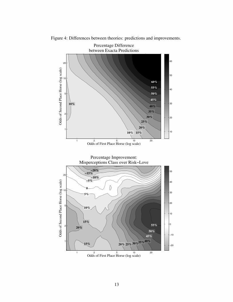
Figure 4: Differences between theories: predictions and improvements.
Odds of First Place Horse (log scale)
Od
ds
of
Sec
on
d P
lace
Ho
rse
(log
sca
le)
Percentage Differencebetween Exacta Predictions
1 2 5 10 20
1
2
5
10
20
10
20
30
40
50
60
10%
10% 15%
20%
25%
30%
35%
40%
45%
50%
55%
60%
Odds of First Place Horse (log scale)
Od
ds
of
Sec
on
d P
lace
Ho
rse
(lo
g s
cale
)
Percentage Improvement:Misperceptions Class over Risk−Love
1 2 5 10 20
1
2
5
10
20
−20
−10
0
10
20
30
40
50
55%
50%
25%20% 30%35%40%
45%
15%
15%
20%
10%
5%
0
−5%
−10%
−15%
−20%
13
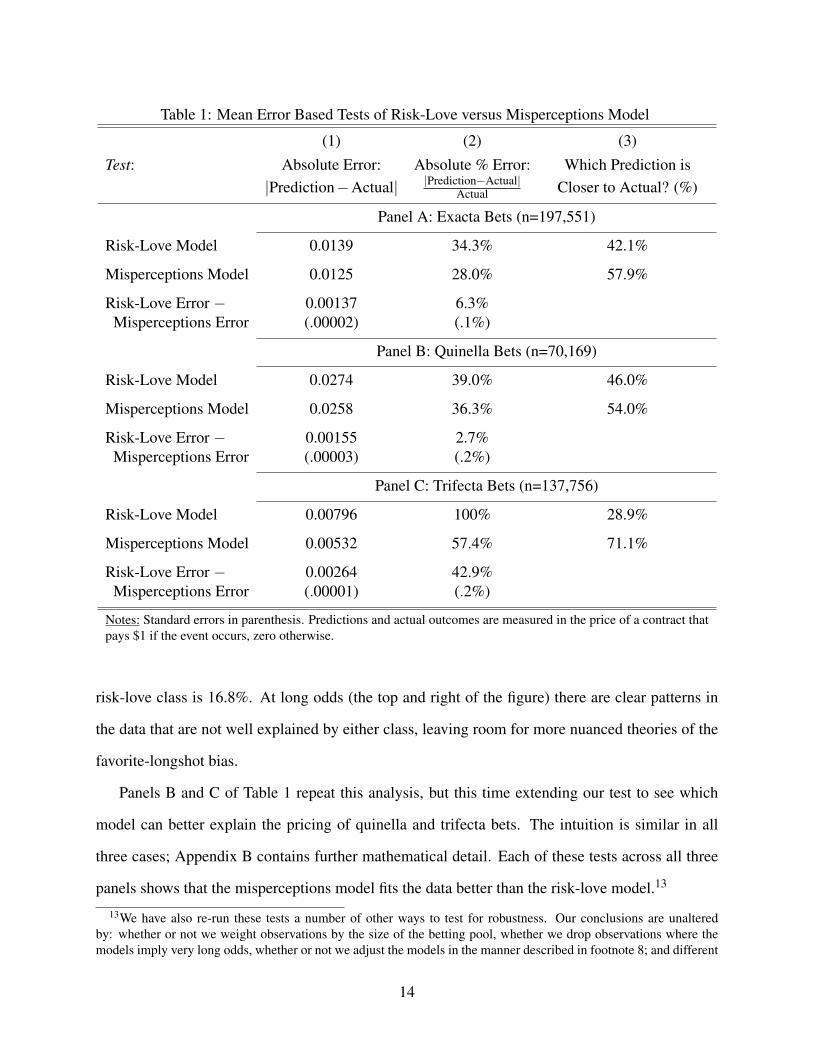
Table 1: Mean Error Based Tests of Risk-Love versus Misperceptions Model
(1) (2) (3)
Test: Absolute Error: Absolute % Error: Which Prediction is|Prediction−Actual| |Prediction−Actual|
Actual Closer to Actual? (%)
Panel A: Exacta Bets (n=197,551)
Risk-Love Model 0.0139 34.3% 42.1%
Misperceptions Model 0.0125 28.0% 57.9%
Risk-Love Error − 0.00137 6.3%Misperceptions Error (.00002) (.1%)
Panel B: Quinella Bets (n=70,169)
Risk-Love Model 0.0274 39.0% 46.0%
Misperceptions Model 0.0258 36.3% 54.0%
Risk-Love Error − 0.00155 2.7%Misperceptions Error (.00003) (.2%)
Panel C: Trifecta Bets (n=137,756)
Risk-Love Model 0.00796 100% 28.9%
Misperceptions Model 0.00532 57.4% 71.1%
Risk-Love Error − 0.00264 42.9%Misperceptions Error (.00001) (.2%)
Notes: Standard errors in parenthesis. Predictions and actual outcomes are measured in the price of a contract thatpays $1 if the event occurs, zero otherwise.
risk-love class is 16.8%. At long odds (the top and right of the figure) there are clear patterns in
the data that are not well explained by either class, leaving room for more nuanced theories of the
favorite-longshot bias.
Panels B and C of Table 1 repeat this analysis, but this time extending our test to see which
model can better explain the pricing of quinella and trifecta bets. The intuition is similar in all
three cases; Appendix B contains further mathematical detail. Each of these tests across all three
panels shows that the misperceptions model fits the data better than the risk-love model.13
13We have also re-run these tests a number of other ways to test for robustness. Our conclusions are unalteredby: whether or not we weight observations by the size of the betting pool, whether we drop observations where themodels imply very long odds, whether or not we adjust the models in the manner described in footnote 8; and different
14

4.1 Relaxing the Assumption of Conditional Independence
Recall that we observe all of the inputs to both pricing models except OB|A, the odds of horse B
finishing second, conditional on horse A winning. In Section 4 we used the convenient assumption
of conditional independence to assess the likely odds of this bet, but there may be good reason
to doubt this assumption. For example, if a heavily favored horse does not win a race, this may
reflect the fact that it was injured during the race, which would imply that it is very unlikely to
come second. That is, the win odds may provide useful guidance on the probability of winning,
but may be a poor guide to the race for second. In this section we test the assumption of conditional
independence and derive two further tests can distinguish between the risk-love and misperceptions
models even if this assumption fails.14
We test the conditional independence assumption by asking whether we can improve on the
predictions of the Harville (1973) formula using other data. As in Section 3.3, the Harville formula
is: pB|A =pB
(1− pA), where pA and pB reflect the probability that horses A and B, respectively, win
the race. We estimate linear probability model where the dependent variable is an indicator variable
for whether horse B finished second. A probit specification yields similar results.
The first specification of Table 2 shows that the Harville formula is an extremely useful pre-
dictor of the probability of a horse finishing second. As a guide for thinking about the explanatory
power of the Harville formula, note that the R2 of specification 1 is about four-fifths the R2 of the
regression of an indicator for whether a horse won the race on its betting odds. Columns 2 and 3
however, provide compelling evidence that we can do better than the Harville formula. Column
2 adds dummy variables representing the odds of the first place horse and the odds of the second
placed horse (using 100 odds groupings in each case, each grouping containing 1% of the odds
distribution). Column 3 includes a full set of interactions of these fixed effects, estimating the
conditional probability non-parametrically from the odds of the first and second place horses; this
regression is equivalent to estimating a large table showing the proportion of horses at odds of
functional forms for the price of a bet, including the natural log price of a $1 claim, the odds, or log-odds.14Even if conditional independence fails, it is not immediately obvious that it yields errors that are correlated in
such as way as to drive our main results. Even so, this is an issue for empirical testing.
15

Table 2: Predicting the Conditional Probability of a Second Place Finish
Dependent Variable: Indicator for whether a horse came in second(Conditional on not winning)
Specification: (1) (2) (3)
Prediction from Conditional Independence 0.793 0.908(Harville Formula) (.0012) (.0077)
Odds of this horse and odds of first horse F=32.3(100 dummy variables for each) p=0.00
Full set of interactions: (this horse ∗ first horse) F=43.5(10,000 dummy variables) p=0.00
R2 0.0782 0.0794 0.0813
Notes: Standard errors in parenthesis. Predictions and actual outcomes are measured in the priceof a contract that pays $1 if the event occurs, zero otherwise.
OB/1 who won the race for second, given the winner was at odds of OA/1. In both columns 2 and
3, F-tests show that these fixed effects are jointly statistically significant.
We now use non-parametrically estimated probabilities as a robustness check of our results in
Table 1. That is, rather than inferring pB|A (and hence π(pB|A) and OB|A) from the Harville formula,
we simply apply the empirical probabilities estimated using the Lowess procedure of Cleveland,
Devlin, and Grosse (1988). We implement this exercise in Table 3, calculating the price of exotic
bets under the risk-love and misperception models, but adapting our earlier approach so that pB|A
is derived from the data.15
The results in Table 3 are almost identical to those in Table 1. For exacta, quinella and trifecta
bets, the misperceptions model has greater explanatory power than the risk-love model.
15Because the precision of our estimates of pB|A vary greatly, WLS weighted by the product of the squared standarderror of pB|A and pA might be appropriate. Additionally, we could estimate pB|A directly from column 3 of Table 2.These approaches produce qualitatively identical results.
16

Table 3: Robustness to Relaxing Conditional Independence Assumption
(1) (2) (3)
Test: Absolute Error: Absolute % Error: Which Prediction is|Prediction−Actual| |Prediction−Actual|
Actual Closer to Actual? (%)
Panel A: Exacta Bets (n=197,551)
Risk-Love Model 0.0117 33.7% 42.9%
Misperceptions Model 0.0109 24.4% 57.1%
Risk-Love Error − 0.00082 9.3%Misperceptions Error (.00001) (.1%)
Panel B: Quinella Bets (n=70,169)
Risk-Love Model 0.0240 37.7% 48.7%
Misperceptions Model 0.0235 33.8% 51.3%
Risk-Love Error − 0.00046 3.9%Misperceptions Error (.00002) (.2%)
Panel C: Trifecta Bets (n=137,756)
Risk-Love Model 0.00650 98.0% 30.4%
Misperceptions Model 0.00464 49.0% 69.6%
Risk-Love Error − 0.00186 49.0%Misperceptions Error (.00001) (.1%)
Notes: Standard errors in parenthesis. Predictions and actual outcomes are measured in the price of a contract thatpays $1 if the event occurs, zero otherwise.
5 Simultaneous Pricing of Exactas and Quinellas
Our final test of the two classes relies only on the relative pricing of exacta and quinella bets, and
is more stringent as it considers these bets simultaneously. 16 As before, we derive predictions
from each class and test which better explains the observed data.
The exacta AB (which represents A winning and B coming second) occurs with probability
pA ∗ pB|A; the BA exacta occurs with probability pB ∗ pA|B. By definition, the corresponding quinella
16Note that these tests are distinct from the work by authors such as Asch and Quandt (1987) and Dolbear (1993),who test whether exacta pricing is arbitrage-linked to win pricing. Instead, we ask whether the same model thatexplains pricing of win bets can jointly explain the pricing of exacta and quinella bets.
17

pays off when the winning exacta is either AB or BA and hence occurs with probability pA ∗ pB|A +
pB ∗ pA|B. Each model yields unique implications for the relative prices of the winning exacta and
quinella bets, and thus unique predictions forpA pB|A
pA pB|A+pB pA|B, which is also the probability horse A
wins given that A and B are the top two finishers. Specifically, consider the AB exacta at odds of
EAB/1, and the corresponding quinella at Q/1:
Risk-Love Class
(Risk-lover, Unbiased expectations)
Exacta: pA pB|AU(EAB) = 1
pB|A =U(OA)U(EAB)
(5)
Quinella: [pA pB|A+ pB pA|B]U(Q) = 1
pA|B = U(OB)(
1U(Q)
− 1U(EAB)
)(7)
Hence from (1), (5) and (7):
pA pB|ApB pA|B+ pA pB|A
=U(Q)
U(EAB)(9)
Misperceptions Class
(Biased expectations, Risk-neutral)
Exacta: π(pA)π(pB|A)(EAB +1) = 1
π(pB|A) =OA +1EAB +1
⇒ pB|A = π-1(
OA +1EAB +1
)(6)
Quinella: [π(pA)π(pB|A)+π(pB)π(pA|B)](Q+1) = 1
π(pA|B) = (OB +1)(
1Q+1 −
1EAB+1
)⇒ pA|B = π -1
((OB+1)(EAB−Q)(EAB+1)(Q+1)
)(8)
Hence from (2), (6) and (8):
pA pB|ApA pB|A+ pB pA|B
=π -1
(1
OA+1
)π -1
(OA+1EAB+1
)π -1
(1
OA+1
)π -1
(OA+1EAB+1
)+π -1
(1
OB+1
)π -1
((OB+1)(EAB−Q)(EAB+1)(Q+1)
) (10)
Equations (9) and (10) show that for any pair of horses at win odds OA/1 and OB/1 with
quinella odds Q/1, each class has different implications for how frequently we expect to observe
the AB exacta winning, relative to the BA exacta. That is, each class gives distinct predictions
about how often a horse with win odds OA/1 will come in first, given that horses with win odds
OA/1 and OB/1 are the top two finishers. As a first test, we regress an indicator for whether the
favorite out of horses A and B actually won, given that horses A and B finished first and second,
on the predictions of each model.17 In this simple specification, the misperceptions class yields a
robust and significant positive correlation with actual outcomes (coefficient = 0.63; standard error
= 0.014, n = 60,288), while the risk-love class is negatively correlated with outcomes (coefficient
=−0.59; standard error = 0.013, n = 60,288).
Where does the perverse negative correlation between the predictions of the risk-love class and
17In the rare event when horses A and B had the same odds we coded the indicator as 0.5.
18
actual outcomes come from? To fix ideas, consider the case where the relative favorite, A, has win
odds of 4/1 and the relative longshot, B, has win odds of 9/1. The data give average exacta odds
EAB = 39/1 and EBA = 44/1 and average quinella odds Q = 20/1. These data agree extremely
closely with the predictions of the misperceptions class, so when (10) is applied to data from such
a race, it makes accurate predictions aboutpA pB|A
pA pB|A+pB pA|B.
Now examine the predictions of the risk-love class. Under this class, an exacta bet at odds
EAB = 39/1 is interpreted as having a large risk penalty, as should be clear from Figures 1 and
3. But if, in fact, compound bets are priced according to the misperceptions class—where bets at
odds of 4/1 and 9/1 do not attract much of a risk (or misperceptions) penalty—then by inferring
the existence of such a penalty, the risk-love model implicitly underestimates the probability that
exacta AB will occur. This underestimation is severe enough that the risk-love class predicts a less
than 50% chance that the relatively favored horse A will finish first out of A and B. But given that
A is the favorite of the two horses (OA/1 = 4/1 < 9/1 = OB/1), it is in fact more likely than not to
finish before B.
If, instead, the relative longshot B wins, the exacta EBA = 44/1 is observed. Applying the
logic above, the risk-love class infers that this price incorporates an even larger risk penalty, and
thus assigns a low probability to this exacta. In turn, this means that it yields a low probability
of horse B coming in first, given that A and B are the top two finishers. However, the risk-love
class will make this prediction only when exacta EBA is observed—that is, horse B actually wins
the race—which is exactly wrong. Thus, conditional on A and B being the top two finishers, the
risk-love class predicts the relative favorite, A, will win with probability less than 12 whenever A
wins. Similarly, whenever B wins, the risk-love class predicts that the relative longshot B will win
with probability less than 12 , and hence predicts that the probability that the relative favorite A wins
is more than 12 . These two forces lead to the perverse negative correlation found above.
The risk-love class fails here because it insists that the same risk-penalty be priced into all bets
of a given risk, regardless of the pool from which the bets are drawn. Yet exotic bets with middling
risk—relative to the other bets available in a given pool—do not tend to attract large risk-penalties,
19

Figure 5: Dropping Conditional Independence
−.5
−.25
0
.25
.5
Act
ual
Ou
tco
mes
Pro
po
rtio
n o
f R
aces
in
wh
ich
Fav
ori
te b
eats
Lo
ng
sho
t
−.5 −.25 0 .25 .5Model Predictions
Proportion where Favorite beats Longshot, Relative to Baseline
Misperceptions Model
Risk Love Model
45 degree line
Proportion of Races in which Favored Horse Beats Longshot, relative to Baseline
Predicting the Winning Exacta Within a Quinella
Notes: Chart shows model predictions from (3) and (4) and actual outcomes relative to a fixed-effect regionbaseline. For the first-two finishing horses the baseline controls for: (a) the odds of the favored horse, (b) theodds of the longshot, (c) the odds of the quinella, and (d) all interactions of (a), (b) and (c). The plot showsmodel predictions after removing fixed effects, rounded to the nearest percentage point, on the x- axis andactual outcomes, relative to the fixed effects, on the y- axis.
even if those bets would be very risky relative to bets in the win pool (Asch and Quandt, 1987).
Note that (9) and (10) also yield distinct predictions of the winning exacta even within any set
of apparently similar races (those whose first two finishers are at OA/1 and OB/1 with the quinella
paying Q/1). Thus, we can include a full set of fixed effects for OA, OB, Q and their interactions
in our statistical tests of the predictions of each class.18 The residual after differencing out these
fixed effects is the predicted likelihood that A beats B, relative to the average for all races in which
a horses at odds of OA/1 and OB/1 fill the quinella at odds Q/1. That is, for all races we compute
the predictions of the likelihood that exacta with the relative favorite winning (AB) occurs, and
18Because the odds OA, OB and Q are actually continuous variables, we include fixed effects for each percentile ofthe distribution of each variable (and a full set of interactions of these fixed effects).
20
subtract the baseline OA ∗OB ∗Q cell mean to yield the predictions for each class of model, relative
to the fixed effects. The results, summarized in Figure 5, are remarkably robust to the inclusion of
these multiple fixed effects (and interactions): the coefficient on the misperceptions class declines
slightly, and insignificantly, while the risk-love class maintains a significant but perversely negative
correlation with outcomes. It should be clear that this test, by focusing only on the relative rankings
of the first two horses, entirely eliminates parametric assumptions about the race for second place.
These tests imply that a model from the risk-love class that accounts for the pricing of win bets
yields inaccurate implications for the relative pricing of exacta and quinella bets. By contrast, the
misperceptions class is consistent with the pricing of exacta, quinella and trifecta bets, and, as this
section shows, also consistent with the relative pricing of exacta and quinella bets. These results
are robust to a range of different approaches to testing the theories.
6 Conclusion
Employing a new dataset which is much larger than those in the existing literature, we document
stylized facts about the rates of return to betting on horses. As with other authors, we note a
substantial favorite-longshot bias. The term bias is somewhat misleading here. That the rate of
return to betting on horses at long odds is much lower than the return to betting on favorites
simply falsifies a model in which bettors maximize a function that is linear in probabilities and
linear in payoffs. Thus, the pricing of win bets can be reconciled by a representative bettor with
either a concave utility function, or a subjective utility function employing non-linear probability
weights that violate the reduction of compound lotteries. For compactness, we referred to the
former as explaining the data with risk-love, while we refer to the latter as explaining the data with
misperceptions. Neither label is particularly accurate as each category includes a wider range of
competing theories.
We show that these classes of models can be separately identified using aggregate data by re-
quiring that they explain both choices over betting on different horses to win and choices over
21

compound bets: exactas, quinellas and trifectas. Because the underlying risk or set of beliefs,
depending on the theory, is traded in both the win and compound betting markets, we can derive
unique testable implications from both sets of theories. Our results are more consistent with the
favorite-longshot bias being driven by misperceptions rather than risk-love. Indeed, while each
class is individually quite useful for pricing compound lotteries, the misperceptions class strongly
dominates the risk-love class. This result is robust to a range of alternative approaches to distin-
guishing between the theories.
This bias likely persists in equilibrium because misperceptions are not large enough to generate
profit opportunities for unbiased bettors. That said, the cost of this bias is also very large, and de-
biasing an individual bettor could reduce their cost of gambling substantially.
22

Appendix DataOur dataset consists of all horse races run in North America from 1992 to 2001. The data was gen-erously provided to us by Axcis Inc., a subsidiary of the jockey club. The data record performanceof every horse in each of its starts, and contains the universe of officially recorded variables havingto do with the horses themselves, the tracks and race conditions.
Our concern is with the pricing of bets. Thus, our primary sample consists of the 6,403,712observations in 865,934 races for which win odds and finishing positions are recorded. We usethese data, subject to the data cleaning restrictions below, to generate Figures 1–3 and 5. We arealso interested in pricing exacta, quinella and trifectas bets and have data on the winning payoffsin 314,977, 116,307 and 282,576 races respectively. The prices of non-winning combinations arenot recorded.
Due to the size of our dataset, whenever observations were problematic, we simply droppedthe entire race from our dataset. Specifically, if a race has more than one horse owned by the sameowner, rather than deal with coupled runners, we simply dropped the race. Additionally, if a racehad a dead heat for first, second or third place the exacta, quinella and trifecta payouts may not beaccurately recorded and so we dropped these races. When the odds of any horse were reported aszero we dropped the race. Further if the odds across all runners implied that the track take was lessthan 15% or more than 22%, we dropped the race. After these steps, we are left with 5,606,336valid observations on win bets from 678,729 races and 1,485,112 observations from 206,808 racesinclude both valid win odds and payoffs for the winning exotic bets.
Appendix Pricing of Compound Lotteries using ConditionalIndependence
In the text we derived the pricing formulae for exacta bets explicitly; this appendix extends thatanalysis to also include the pricing of quinella and trifecta bets. The derivations of these pricingformulae depend on the following two formulae originally derived in Section 3:
Risk-Love Model
(Risk-lover, Unbiased expectations)
U(O) =1p
(11)
Misperceptions Model
(Biased expectations, Risk-neutral)
π(p) =1
O+1(12)
As in the text, we derive pricing formulae by imposing that the expected utility of all bets isequal. Consider a horse race which includes horses A, B and C. An exacta requires the bettor tocorrectly specify the first two horses, in order. A quinella is a bet on two horses to finish first andsecond, but the bettor need not specify their order. A quinella bet on horses A and B gives oddsQAB. A trifecta is a bet on three horses to finish first, second and third, and the bettor must correctlyspecify their order. A trifecta bet on horses A, B and C, in that order, gives odds TABC. Thus thequinella and trifecta analogues to equations (3) and (4) in the main text are:
23

Risk-Love Model
(Risk-lover, Unbiased expectations)
Quinella:
[pA pB|A + pB pA|B]U(QAB) = 1
QAB = U−1(
U(OA)U(OB|A)U(OB)U(OA|B)U(OA)U(OB|A)+U(OB)U(OA|B)
)(3q)
Trifecta:
pA pB|A pC|A,BU(TABC) = 1
TABC = U -1(U(OA)U(OB|A)U(OC|A,B))
(3t)
Risk-Love Model
(Risk-lover, Unbiased expectations)
Quinella:
[π(pA)π(pB|A)+π(pB)π(pA|B)](QAB +1) = 1
QAB =(OA+1)(OB|A)(OB+1)(OA|B)
(OA+1)(OB|A)+(OB+1)(OA|B) (4q)
Trifecta:
π(pA)π(pB|A)π(pC|A,B)(TABC +1) = 1
TABC = (OA +1)(OB|A +1)(OC|A,B +1)−1 (4t)
The odds data, OA, OB and OC are directly observable. The utility U(·) and probability weight-ing π(·) functions that we use are shown in Figure 3. In order to price these compound bets wealso need the conditional probabilities OB|A, OA|B and OC|A,B.
As noted in Section 3.3, we provide two approaches to recovering these unobservables. First,we assume conditional independence, as in Harville (1973). Thus, pB|A = pB/(1− pA), pA|B =pA/(1− pB) and pC|A,B = pC/(1− pA− pB). Our second approach directly estimates pB|A, pA|B, andpC|A,B using Lowess smoothing as described in Cleveland, Devlin, and Grosse (1988). Under boththe Harville and Lowess approach these probability estimates and (11) and (12) are used to recoverthe relevant odds OB|A, OA|B and OC|A,B.
24
ReferencesAczel, J. 1966. Lectures on Functional Equations and their Applications. New York: Academic
Press.
Ali, Mukhtar M. 1977. “Probability and Utility Estimates for Racetrack Bettors.” The Journal ofPolitical Economy 85 (4):803–815.
———. 1979. “Some Evidence of the Efficiency of a Speculative Market.” Econometrica47 (2):387–392.
Asch, Peter, Burton G. Malkiel, and Richard E. Quandt. 1982. “Racetrack Betting and InformedBehavior.” Journal of Financial Economics 10 (2):187–194.
Asch, Peter and Richard E. Quandt. 1987. “Efficiency and Profitability in Exotic Bets.” Economica54 (215):289–298.
Busche, Kelly. 1994. ““Efficient Market Results in an Asian Setting”.” In Efficiency of RacetrackBetting Markets, edited by Donald Hausch, V. Lo, and William T. Ziemba. New York: AcademicPress, 615–616.
Busche, Kelly and Christopher D. Hall. 1988. “An Exception to the Risk Preference Anomaly.”The Journal of Business 61 (3):337–346.
Camerer, Colin F. and Teck Hua Ho. 1994. “Violations of the betweenness axiom and nonlinearityin probability.” Journal of Risk and Uncertainty 8 (2):167–196.
Cleveland, William S., Susan J. Devlin, and Eric Grosse. 1988. “Regression by Local Fitting:Methods, Properties, and Computational Algorithms.” Journal of Econometrics 37 (1):87–114.
Conlisk, John. 1993. “The Utility of Gambling.” Journal of Risk and Uncertainty 6 (3):255–275.
Dolbear, F. Trenery. 1993. “Is Racetrack Betting on Exactas Efficient?” Economica 60 (237):105–111.
Friedman, Milton and Leonard J. Savage. 1948. “The Utility Analysis of Choices Involving Risk.”The Journal of Political Economy 56 (4):279–304.
Gabriel, Paul E. and James R. Marsden. 1990. “An Examination of Market Efficiency in BritishRacetrack Betting.” The Journal of Political Economy 98 (4):874–885.
Gandhi, Amit. 2007. “Rational Expectations at the Racetrack: Testing Expected Utility UsingPrediction Market Prices.” University of Wisconsin-Madison, mimeo.
Golec, Joseph and Maurry Tamarkin. 1998. “Bettors Love Skewness, Not Risk, at the HorseTrack.” Journal of Political Economy 106 (1):205.
Griffith, R.M. 1949. “Odds Adjustments by American Horse-Race Bettors.” The American Journalof Psychology 62 (2):290–294.
25
Harville, David A. 1973. “Assigning Probabilities to the Outcomes of Multi-Entry Competitions.”Journal of the American Statistical Association 68 (342):312–316.
Henery, Robert J. 1985. “On the Average Probability of Losing Bets on Horses with Given StartingPrice Odds.” Journal of the Royal Statistical Society. Series A (General) 148 (4):342–349.
Hurley, William and Lawrence McDonough. 1995. “A Note on the Hayek Hypothesis and theFavorite-Longshot Bias in Parimutuel Betting.” The American Economic Review 85 (4):949–955.
Jullien, Bruno and Bernard Salanie. 2000. “Estimating Preferences Under Risk: The Case ofRacetrack Bettors.” Journal of Political Economy 108 (3):503.
Kahneman, Daniel and Amos Tversky. 1979. “Prospect Theory: An Analysis of Decision underRisk.” Econometrica 47 (2):263–292.
Levitt, Steven D. 2004. “Why are Gambling Markets Organised so Differently from FinancialMarkets?” The Economic Journal 114 (495):223–246.
Manski, Charles F. 2006. “Interpreting the Predictions of Prediction Markets.” Economics Letters91 (3):425–429.
McGlothlin, William H. 1956. “Stability of Choices among Uncertain Alternatives.” The AmericanJournal of Psychology 69 (4):604–615.
Ottaviani, Marco and Peter Norman Sørenson. 2009. “Noise, Information, and the Favorite-Longshot Bias in Parimutuel Predictions.” American Economic Journal: Microeconomics forth-coming.
Prelec, Drazen. 1998. “The Probability Weighting Function.” Econometrica 66 (3):497–527.
Quandt, Richard E. 1986. “Betting and Equilibrium.” The Quarterly Journal of Economics101 (1):201–208.
Rosett, Richard N. 1965. “Gambling and Rationality.” The Journal of Political Economy73 (6):595–607.
Samuelson, Paul A. 1952. “Probability, Utility, and the Independence Axiom.” Econometrica20 (4):670–678.
Sauer, Raymond D. 1998. “The Economics of Wagering Markets.” Journal of Economic Literature36 (4):2021–2064.
Segal, Uzi. 1990. “Two-Stage Lotteries without the Reduction Axiom.” Econometrica 58 (2):349–377.
Shin, Hyun Song. 1992. “Prices of State Contingent Claims with Insider Traders, and theFavourite-Longshot Bias.” The Economic Journal 102 (411):426–435.
26
Snowberg, Erik and Justin Wolfers. 2007. ““The Favorite-Longshot Bias: Understanding a MarketAnomaly”.” In Efficiency of Sports and Lottery Markets, edited by Donald Hausch and WilliamZiemba. Elsevier: Handbooks in Finance series.
Thaler, Richard H. and William T. Ziemba. 1988. “Anomalies: Parimutuel Betting Markets: Race-tracks and Lotteries.” The Journal of Economic Perspectives 2 (2):161–174.
Weitzman, Martin. 1965. “Utility Analysis and Group Behavior: An Empirical Study.” The Jour-nal of Political Economy 73 (1):18–26.
Williams, Leighton Vaughn and David Paton. 1997. “Why is There a Favourite-Longshot Bias inBritish Racetrack Betting Markets?” The Economic Journal 107 (440):150–158.
27


