Financial Intermediaries and Markets

Franklin AllenDepartment of FinanceWharton School

University of PennsylvaniaPhiladelphia, PA 19104allenf@wharton.upenn.edu

Douglas GaleDepartment of EconomicsNew York University269 Mercer StreetNew York, NY 10003douglas.gale@nyu.edu

December 19, 2003

Abstract

A complex financial system comprises both financial markets and financial intermediaries.We distinguish financial intermediaries according to whether they issue complete contingentcontracts or incomplete contracts. Intermediaries such as banks that issue incomplete con-tracts, e.g., demand deposits, are subject to runs, but this does not imply a market failure.A sophisticated financial system–a system with complete markets for aggregate risk andlimited market participation–is incentive-efficient, if the intermediaries issue complete con-tingent contracts, or else constrained-efficient, if they issue incomplete contracts. We arguethat there may be a role for regulating liquidity provision in an economy in which marketsfor aggregate risks are incomplete.

1 Markets, intermediaries and crises

For a long time, it has been taken as axiomatic that financial crises are best avoided. Weconfront this conventional wisdom by showing that, under certain conditions, a laisser-fairefinancial system achieves the incentive-efficient or constrained-efficient allocation.1 Further-more, constrained efficiency may require financial crises in equilibrium. The assumptionsneeded to achieve these efficiency results are restrictive, but no more so than the assump-tions normally required to ensure Pareto-efficiency of Walrasian equilibrium. The importantpoint is that optimality of avoiding crises should not be taken as axiomatic. If regulationis required to minimize or obviate the costs of financial crises, it should be justified by amicroeconomic welfare analysis based on standard assumptions. Furthermore, the form ofthe intervention should be derived from microeconomic principles. Financial institutionsand financial markets exist to facilitate the efficient allocation of risks and resources. Anygovernment intervention will have an impact on the normal functioning of the financial sys-tem. A policy of preventing financial crises will inevitably create distortions. One of theadvantages of a microeconomic analysis of financial crises is that it clarifies the costs andbenefits of these distortions.Policy analyses of banking and securities markets tend to be based on very specific mod-

els.2 In the absence of a general equilibrium framework, it is hard to evaluate the robustnessof the results and, ultimately, to answer the question: What precisely are the market failuresassociated with financial crises? In this paper, we take a step toward developing a generalmodel to analyze market failures in the financial sector and study a complex, decentral-ized, financial system comprising both financial markets and financial intermediaries.3 Forthe most part, the seminal models of bank runs, such as Bryant (1980) and Diamond andDybvig (1983), analyze the behavior of a single bank and consist of a contracting problemfollowed by a coordination problem.4 We combine recent developments in the theory of bank-

1Wallace (1990) suggests that bank runs might be efficient. Examples of efficient bank runs were providedby Alonso (1996) and Allen and Gale (1998). Here we provide general sufficient conditions for the efficiencyof financial crises.

2See Bhattacharya and Thakor (1993) for a survey. For examples of more recent work that stresses theanalysis of welfare, see Matutes and Vives (1996, 2000).

3In this paper we use the term “financial markets” narrowly to denote markets for securities. Otherauthors have allowed for markets in which mechanisms are traded (e.g., Bisin and Gottardi (2000)). Weprefer to call this intermediation. Formally, the two activities are similar, but in practice the economicinstitutions are quite different.

4Early models of financial crises were developed in the 1980s by Bryant (1980) and Diamond and Dybvig(1983). Important contributions were also made by Chari and Jagannathan (1988), Chari (1989), Champ,Smith, and Williamson (1996), Jacklin (1986), Jacklin and Bhattacharya (1988), Postlewaite and Vives(1986), Wallace (1988; 1990) and others. Theoretical research on speculative currency attacks, bankingpanics, the role of liquidity and contagion have taken a number of approaches. One is built on the foundationsprovided by early research on bank runs (e.g., Hellwig (1994; 1998), Diamond (1997), Allen and Gale (1998;1999; 2000a; 2000b), Peck and Shell (1999), Chang and Velasco (2000; 2001)) and Diamond and Rajan(2001)). Other approaches include those based on macroeconomic models of currency crises that developedfrom the insights of Krugman (1979), Obstfeld (1986) and Calvo (1988) (see, e.g., Corsetti, Pesenti, andRoubini (1999) for a recent contribution and Flood and Marion (1999) for a survey), game theoretic models

1

ing with further innovations to model a complex financial system. The model has severalinteresting features: it introduces markets into a general-equilibrium theory of institutions;it endogenizes the cost of forced liquidation;5 it allows for a fairly general specification of theeconomic environment; it allows for interaction between liquidity and asset pricing;6 and itallows us to analyze the regulation of the financial system using the standard tools of welfareeconomics.In our model, intermediaries have two functions. Following Diamond and Dybvig (1983),

intermediaries are providers of insurance services. By pooling the assets of individuals withuncertain preference for liquidity they can provide a higher degree of liquidity for any givenlevel of returns on the portfolio. Their second function is to provide risk sharing services bypackaging existing claims on behalf of investors who do not have access to markets. In thisrespect the intermediary operates more like a mutual fund, but both functions are essentialto the operation of an optimal intermediary. Financial intermediaries have many otherfunctions, of course, including payments, information gathering, lending, and underwriting,but we ignore these for the purpose of focusing on risk sharing and macroeconomic stability.We distinguish between intermediaries that can offer complete contingent contracts and

intermediaries that can only offer incomplete contracts. An example of the latter would bebanks that can only offer deposit contracts. With complete contracts, the consequences ofdefault can be anticipated and included in the contract, so without loss of generality we canassume default does not occur. With incomplete contracts, however, default can improvewelfare by increasing the contingency of the contract (see, for example, Zame (1993)).Aggregate risk in our model takes the form of shocks to asset returns and preferences.

Formally, there is a finite set of aggregate states of nature that determines asset returns andpreferences. We contrast economies with complete markets, in which there is a complete setof Arrow securities, one for each aggregate state, from economies with incomplete markets, inwhich the set of Arrow securities is less than the number of aggregate states. This producesa 2× 2 classification of models, according to the completeness of contracts and markets.

Complete markets Incomplete marketsComplete contracts incentive-efficient not efficientIncomplete contracts constrained-efficient not efficient

Financial crises do occur in our model, but are not necessarily a source of market failure. Asophisticated financial system provides optimal liquidity and risk sharing, where a financialsystem is “sophisticated” if markets for aggregate risks are complete and market participation

(see Morris and Shin (1998), Morris (2000) and Morris and Shin (2000) for an overview), amplificationmechanisms (e.g., Cole and Kehoe (2000) and Chari and Kehoe (2000)) and the borrowing of foreign currencyby firms (e.g., Aghion, Bacchetta and Banerjee (2000)).

5Most of the literature, following Diamond and Dybvig (1983), assumes the existence of a technology forliquidating projects. Here we assume that a financially distressed institution sells assets to other institutions.This realistic feature of the model has important implications for welfare analysis. Ex post, liquidation doesnot entail a deadweight cost because assets are merely transferred from one owner to another. Ex ante,liquidation can result in inefficient risk sharing, but only if markets for hedging the risk are incomplete.

6In particular, there is a role for cash-in-the-market pricing (Allen and Gale (1994)).

2

is incomplete. Efficiency depends on the completeness of markets but does not depend onwhether contracts are complete or incomplete.These results provide a benchmark for evaluating government intervention and regula-

tion. If a sophisticated financial system leads to an incentive-efficient or constrained-efficientallocation, what precisely is the role of the government or central bank in intervening in thefinancial system? What can the government or central bank do that private institutions andthe market cannot do? Our efficiency theorem assumes that markets for aggregate risk arecomplete. Missing markets may provide a role for government intervention.In addition, the model provides some important insights into the working of complex

financial systems. We include a series of examples to illustrate the properties of the model.In particular, we show that, in some cases, (a) existence and optimality require that equilibriabe “mixed”, that is, identical banks choose very different risk strategies; (b) default and crisesare optimal when markets are complete and contracts incomplete; (c) asset pricing in a crisisis determined by the amount of liquidity in the market as well as by the asset returns; and(d) risk sharing is suboptimal with incomplete markets.Our results are related to a small but important literature that seeks to extend the

traditional intermediation literature in a more general equilibrium direction. Von Thadden(1999) also studies an integrated model of demand deposits and anonymous markets. Martin(2000) addresses the question of whether liquidity provision by the central bank can preventcrises without creating a moral hazard problem. Gromb and Vayanos (2001) study assetpricing in a model of collateralized arbitrage.The rest of the paper is organized as follows. Section 2 describes the primitives of the

model. Section 3 explores the welfare properties of liquidity provision and risk sharing in thecontext of an economy with a sophisticated financial system in which institutions take theform of general intermediaries. Section 4 shows that incomplete participation is critical forthe optimality results achieved in the previous two sections. Section 5 extends this analysisto an economy with a sophisticated financial system in which institutions use incompletecontracts. In Section 6, we consider an economy with incomplete markets and characterizethe conditions under which welfare can be increased by in some cases increasing and in somecases decreasing liquidity. Section 7 contains some final remarks and some of the proofs aregathered together in Section 8.

2 The basic economy

There are three dates t = 0, 1, 2 and a single good at each date. The good is used forconsumption and investment.The economy is subject to two kinds of uncertainty. First, individual agents are subject

to idiosyncratic preference shocks, which affect their demand for liquidity (these will bedescribed later). Second, the entire economy is subject to aggregate shocks that affectasset returns and the cross-sectional distribution of preferences. The aggregate shocks arerepresented by a finite number of states of nature, indexed by η ∈ H. At date 0, all agentshave a common prior probability density ν(η) over the states of nature. All uncertainty is

3

resolved at the beginning of date 1, when the state η is revealed and each agent discovershis individual preference shock.Each agent has an endowment of one unit of the good at date 0 and no endowment at

dates 1 and 2. So, in order to provide consumption at dates 1 and 2, they need to invest.There are two assets distinguished by their returns and liquidity structure. One is a

short-term asset (the short asset), and the other is a long-term asset (the long asset). Theshort asset is represented by a storage technology: one unit invested in the short asset atdate t = 0, 1 yields a return of one unit at date t+1. The long asset yields a return after twoperiods. One unit of the good invested in the long asset at date 0 yields a random return ofR(η) > 1 units of the good at date 2 if state η is realized.Investors’ preferences are distinguished ex ante and ex post. At date 0 there is a finite

number n of types of investors, indexed by i = 1, ..., n. We call i an investor’s ex ante type.An investor’s ex ante type is common knowledge and hence contractible. The measure ofinvestors of type i is denoted by µi > 0. The total measure of investors is normalized to oneso that

Pi µi = 1.

While investors of a given ex ante type are identical at date 0, they receive a private,idiosyncratic, preference shock at the beginning of date 1. The date 1 preference shock isdenoted by θi ∈ Θi, where Θi is a finite set. We call θi the investor’s ex post type. Becauseθi is private information, contracts cannot be explicitly contingent on θi.Investors only value consumption at dates 1 and 2. An investor’s preferences are rep-

resented by a von Neumann-Morgenstern utility function, ui(c1, c2; θi), where ct denotesconsumption at date t = 1, 2. The utility function ui(·; θi) is assumed to be concave, increas-ing, and continuous for every type θi. Diamond and Dybvig (1983) assumed that consumerswere one of two ex post types, either early diers who valued consumption at date 1 or latediers who valued consumption at date 2. This is a special case of the preference shock θi.The present framework allows for much more general preference uncertainty.The probability of being an investor of type (i, θi) conditional on state η is denoted by

λi(θi, η) > 0. The probability of being an agent of type i is µi. Consistency therefore requiresthat X

θi

λi(θi, η) = µi,∀η ∈ H.

By the usual “law of large numbers” convention, the cross-sectional distribution of types isassumed to be the same as the probability distribution λ. We can therefore interpret λi(θi, η)as the number of agents of type (i, θi) in state η.

3 Optimal intermediation

Intermediaries have two broad functions in this model. First, because individual investorsdo not have access to markets for sharing aggregate risk, intermediaries trade existing claimson their behalf to produce a synthetic risk-sharing contract for the investors. In this respect,they are like mutual funds. Secondly, as in the Diamond-Dybvig model, intermediaries

4

provide investors with insurance against the preference shocks. One difference from theDiamond-Dybvig model is that intermediaries cannot physically liquidate projects whenthey need liquidity. Instead, they sell assets on the capital market at date 1. Because theiris no physical cost of liquidating assets, liquidation is ex post efficient: the buyer’s loss isthe seller’s gain and vice versa.In this section we assume that financial institutions take the form of general interme-

diaries. Each intermediary offers a single contract and each ex ante type is attracted to adifferent intermediary. Contracts are contingent on the aggregate states η and individuals’reports of their ex post types, subject to incentive compatibility constraints.One can, of course, imagine a world in which a single “universal” intermediary offers

contracts to all ex ante types of investors. A universal intermediary could act as a centralplanner and implement the first-best allocation of risk. There would be no reason to resortto markets at all. Our world view is based on the assumption that transaction costs precludethis kind of centralized solution and that decentralized intermediaries are restricted in thenumber of different contracts they can offer. This assumption provides a role for financialmarkets in which financial intermediaries can share risk and obtain liquidity.At the same time, financial markets alone will not suffice to achieve optimal risk sharing.

Because individual economic agents have private information, markets for individual risks areincomplete. The markets that are available will not achieve an incentive-efficient allocationof risk. Intermediaries, by contrast, can offer individuals incentive-compatible contracts andimprove on the risk sharing provided by the market.In the Diamond-Dybvig (1983) model, all investors are ex ante identical. Consequently,

a single representative bank can provide complete risk sharing and there is no need formarkets to provide cross-sectional risk sharing across banks. Allen and Gale (1994) showedthat differences in risk and liquidity preferences can be crucial in explaining asset prices.This is another reason for allowing for ex ante heterogeneity.

3.1 Markets

At date 0 investors deposit their endowments with an intermediary in exchange for a generalrisk sharing contract. The intermediaries have access to a complete set of Arrow securitiesmarkets at date 0. For each aggregate state η there is a security traded at date 0 thatpromises one unit of the good at date 1 if state η is observed and nothing otherwise. Letq(η) denote the price of one unit of the Arrow security corresponding to state η, that is, thenumber of units of the good at date 0 needed to buy one unit of the good in state η at date1.All uncertainty is resolved at the beginning of date 1. Consequently there is no need

to trade contingent securities at date 1. Instead, we assume there is a spot market and aforward market for the good at date 1. The good at date 1 is the numeraire so p1(η) = 1;the price of the good at date 2 for sale at date 1 is denoted by p2(η), i.e., p2(η) is the numberof units of the good at date 1 needed to purchase one unit of the good at date 2 in state η.Let p(η) = (p1(η), p2(η)) = (1, p2(η)) denote the vector of goods prices at date 1 in state η.

5

Note that we do not assume the existence of a technology for physically liquidatingprojects. Instead, we follow Allen and Gale (1998) in assuming that an institution in distresssells long-term assets to other institutions. From the point of view of the economy as a whole,the long-term assets cannot be liquidated–someone has to hold them.

3.2 Intermediation mechanisms

Investors participate in markets indirectly, through intermediaries. An intermediary is arisk-sharing institution that invests in the short and long assets on behalf of investors andprovides them with consumption at dates 1 and 2. Intermediaries use markets to hedge therisks that they manage for investors.Each investor of type i gives his endowment (one unit of the good) to an intermediary

of type i at date 0. In exchange, he gets a bundle of goods xi(θi, η) ∈ R2+ at dates 1 and 2

in state η if he reports the ex post type θi. In effect, the function xi = {xi(θi, η)} is a directmechanism that maps agents’ reports into feasible consumption allocations.7

A feasible mechanism is incentive-compatible. The appropriate definition of the incentive-compatibility constraint must take into account the fact that agents can use the short assetto store the good from date 1 to date 2. Suppose that the agent receives a consumptionbundle xi(θi, η) from the intermediary. By saving, he can obtain any consumption bundlec ∈ R2

+ such that

c1 ≤ xi1(θi, η),2X

t=1

ct ≤2X

t=1

xit(θi, η). (1)

Let C(xi(θi, η)) denote the set of consumption bundles satisfying (1). The maximum util-ity that can be obtained from the consumption bundle xi(θi, η) by saving is denoted byu∗i (xi(θi, η), θi) and defined by

u∗i (xi(θi, η), θi) = sup {ui(c, θi) : c ∈ C(xi(θi, η))} .Then the incentive constraint with saving can be written as:

ui(xi(θi, η), θi) ≥ u∗i (xi(θi, η), θi),∀θi, θi ∈ Θi, ∀η ∈ H. (2)

Notice that by placing ui(·) on the left hand side of (2), we ensure that even a truth-tellingagent will not want to save outside of the intermediary. There is no loss of generality in thisrestriction, since the intermediary can tailor the timing of consumption to the agent’s needs.Let Xi denote the set of incentive-compatible mechanisms when the depositor has access tothe storage technology.

7A direct mechanism is normally a function that assigns a unique outcome to each profile of types chosenby the investors. In a symmetric direct mechanism, the outcome for a single investor depends only onthe individual’s report and the distribution of reports by other investors. In a truth-telling equilibrium,the reports of other investors are given by the distribution λ(·, η) so a symmetric direct mechanism shouldproperly be written xi(θi, λ(·, η), η) but since λ(·, η) is given as a function of η there is no loss of generalityin suppressing the reference to λ(·, η).

6

3.3 Equilibrium

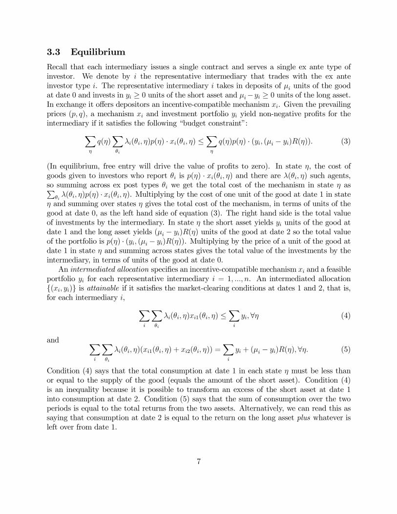
Recall that each intermediary issues a single contract and serves a single ex ante type ofinvestor. We denote by i the representative intermediary that trades with the ex anteinvestor type i. The representative intermediary i takes in deposits of µi units of the goodat date 0 and invests in yi ≥ 0 units of the short asset and µi−yi ≥ 0 units of the long asset.In exchange it offers depositors an incentive-compatible mechanism xi. Given the prevailingprices (p, q), a mechanism xi and investment portfolio yi yield non-negative profits for theintermediary if it satisfies the following “budget constraint”:X

η

q(η)Xθi

λi(θi, η)p(η) · xi(θi, η) ≤Xη

q(η)p(η) · (yi, (µi − yi)R(η)). (3)

(In equilibrium, free entry will drive the value of profits to zero). In state η, the cost ofgoods given to investors who report θi is p(η) · xi(θi, η) and there are λ(θi, η) such agents,so summing across ex post types θi we get the total cost of the mechanism in state η asP

θiλ(θi, η)p(η) · xi(θi, η). Multiplying by the cost of one unit of the good at date 1 in state

η and summing over states η gives the total cost of the mechanism, in terms of units of thegood at date 0, as the left hand side of equation (3). The right hand side is the total valueof investments by the intermediary. In state η the short asset yields yi units of the good atdate 1 and the long asset yields (µi − yi)R(η) units of the good at date 2 so the total valueof the portfolio is p(η) · (yi, (µi − yi)R(η)). Multiplying by the price of a unit of the good atdate 1 in state η and summing across states gives the total value of the investments by theintermediary, in terms of units of the good at date 0.An intermediated allocation specifies an incentive-compatible mechanism xi and a feasible

portfolio yi for each representative intermediary i = 1, ..., n. An intermediated allocation{(xi, yi)} is attainable if it satisfies the market-clearing conditions at dates 1 and 2, that is,for each intermediary i, X

i

Xθi

λi(θi, η)xi1(θi, η) ≤Xi

yi,∀η (4)

and Xi

Xθi

λi(θi, η)(xi1(θi, η) + xi2(θi, η)) =Xi

yi + (µi − yi)R(η), ∀η. (5)

Condition (4) says that the total consumption at date 1 in each state η must be less thanor equal to the supply of the good (equals the amount of the short asset). Condition (4)is an inequality because it is possible to transform an excess of the short asset at date 1into consumption at date 2. Condition (5) says that the sum of consumption over the twoperiods is equal to the total returns from the two assets. Alternatively, we can read this assaying that consumption at date 2 is equal to the return on the long asset plus whatever isleft over from date 1.

7

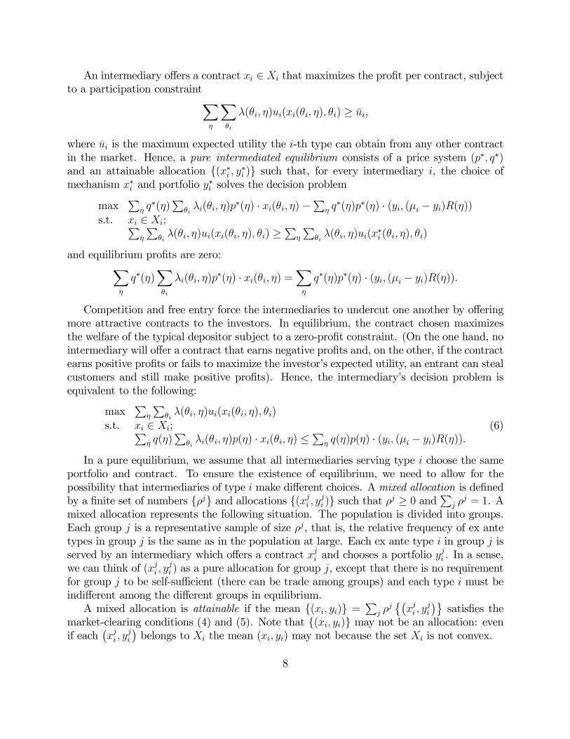
An intermediary offers a contract xi ∈ Xi that maximizes the profit per contract, subjectto a participation constraintX

η

Xθi

λ(θi, η)ui(xi(θi, η), θi) ≥ ui,

where ui is the maximum expected utility the i-th type can obtain from any other contractin the market. Hence, a pure intermediated equilibrium consists of a price system (p∗, q∗)and an attainable allocation {(x∗i , y∗i )} such that, for every intermediary i, the choice ofmechanism x∗i and portfolio y

∗i solves the decision problem

maxP

η q∗(η)

Pθiλi(θi, η)p

∗(η) · xi(θi, η)−P

η q∗(η)p∗(η) · (yi, (µi − yi)R(η))

s.t. xi ∈ Xi;Pη

Pθiλ(θi, η)ui(xi(θi, η), θi) ≥

Pη

Pθiλ(θi, η)ui(x

∗i (θi, η), θi)

and equilibrium profits are zero:Xη

q∗(η)Xθi

λi(θi, η)p∗(η) · xi(θi, η) =

Xη

q∗(η)p∗(η) · (yi, (µi − yi)R(η)).

Competition and free entry force the intermediaries to undercut one another by offeringmore attractive contracts to the investors. In equilibrium, the contract chosen maximizesthe welfare of the typical depositor subject to a zero-profit constraint. (On the one hand, nointermediary will offer a contract that earns negative profits and, on the other, if the contractearns positive profits or fails to maximize the investor’s expected utility, an entrant can stealcustomers and still make positive profits). Hence, the intermediary’s decision problem isequivalent to the following:

maxP

η

Pθiλ(θi, η)ui(xi(θi, η), θi)

s.t. xi ∈ Xi;Pη q(η)

Pθiλi(θi, η)p(η) · xi(θi, η) ≤

Pη q(η)p(η) · (yi, (µi − yi)R(η)).

(6)

In a pure equilibrium, we assume that all intermediaries serving type i choose the sameportfolio and contract. To ensure the existence of equilibrium, we need to allow for thepossibility that intermediaries of type i make different choices. A mixed allocation is definedby a finite set of numbers {ρj} and allocations {(xji , yji )} such that ρj ≥ 0 and

Pj ρ

j = 1. Amixed allocation represents the following situation. The population is divided into groups.Each group j is a representative sample of size ρj, that is, the relative frequency of ex antetypes in group j is the same as in the population at large. Each ex ante type i in group j isserved by an intermediary which offers a contract xji and chooses a portfolio y

ji . In a sense,

we can think of (xji , yji ) as a pure allocation for group j, except that there is no requirement

for group j to be self-sufficient (there can be trade among groups) and each type i must beindifferent among the different groups in equilibrium.A mixed allocation is attainable if the mean {(xi, yi)} =

Pj ρ

j©¡xji , y

ji

¢ªsatisfies the

market-clearing conditions (4) and (5). Note that {(xi, yi)} may not be an allocation: evenif each

¡xji , y

ji

¢belongs to Xi the mean (xi, yi) may not because the set Xi is not convex.

8

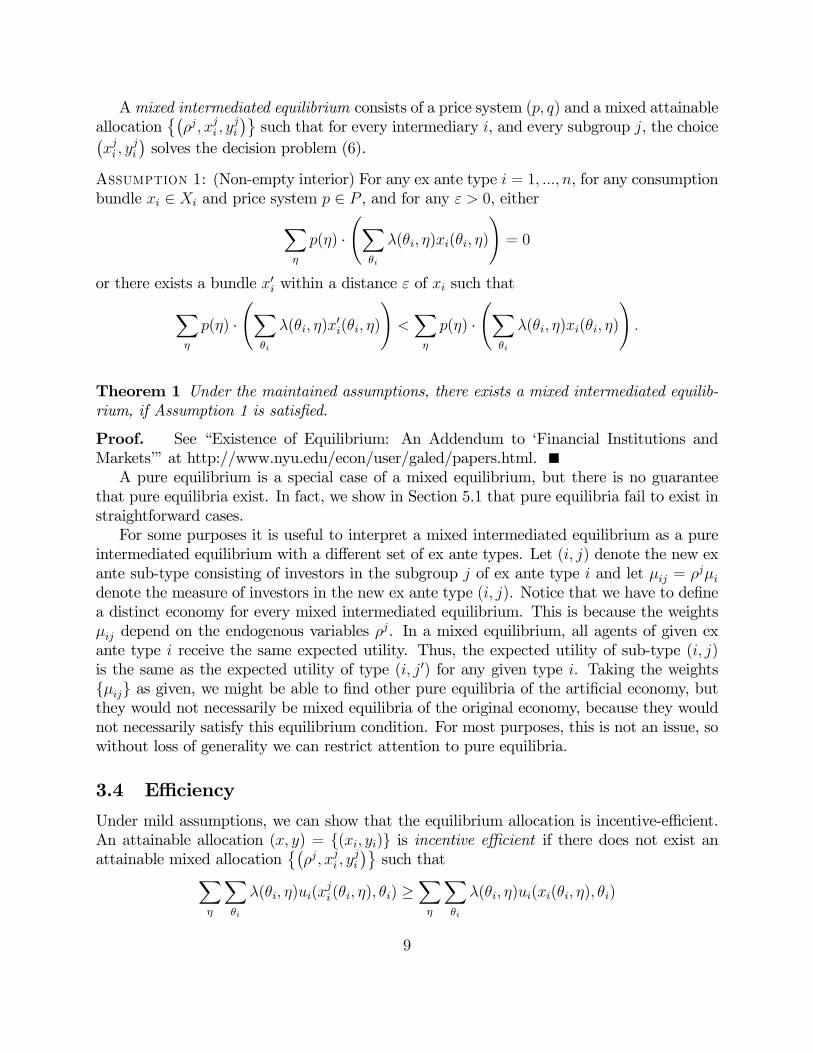
Amixed intermediated equilibrium consists of a price system (p, q) and a mixed attainableallocation

©¡ρj, xji , y

ji

¢ªsuch that for every intermediary i, and every subgroup j, the choice¡

xji , yji

¢solves the decision problem (6).

Assumption 1: (Non-empty interior) For any ex ante type i = 1, ..., n, for any consumptionbundle xi ∈ Xi and price system p ∈ P , and for any ε > 0, eitherX

η

p(η) ·ÃX

θi

λ(θi, η)xi(θi, η)

!= 0

or there exists a bundle x0i within a distance ε of xi such thatXη

p(η) ·ÃX

θi

λ(θi, η)x0i(θi, η)

!<Xη

p(η) ·ÃX

θi

λ(θi, η)xi(θi, η)

!.

Theorem 1 Under the maintained assumptions, there exists a mixed intermediated equilib-rium, if Assumption 1 is satisfied.

Proof. See “Existence of Equilibrium: An Addendum to ‘Financial Institutions andMarkets’” at http://www.nyu.edu/econ/user/galed/papers.html.A pure equilibrium is a special case of a mixed equilibrium, but there is no guarantee

that pure equilibria exist. In fact, we show in Section 5.1 that pure equilibria fail to exist instraightforward cases.For some purposes it is useful to interpret a mixed intermediated equilibrium as a pure

intermediated equilibrium with a different set of ex ante types. Let (i, j) denote the new exante sub-type consisting of investors in the subgroup j of ex ante type i and let µij = ρjµidenote the measure of investors in the new ex ante type (i, j). Notice that we have to definea distinct economy for every mixed intermediated equilibrium. This is because the weightsµij depend on the endogenous variables ρ

j. In a mixed equilibrium, all agents of given exante type i receive the same expected utility. Thus, the expected utility of sub-type (i, j)is the same as the expected utility of type (i, j0) for any given type i. Taking the weights{µij} as given, we might be able to find other pure equilibria of the artificial economy, butthey would not necessarily be mixed equilibria of the original economy, because they wouldnot necessarily satisfy this equilibrium condition. For most purposes, this is not an issue, sowithout loss of generality we can restrict attention to pure equilibria.

3.4 Efficiency

Under mild assumptions, we can show that the equilibrium allocation is incentive-efficient.An attainable allocation (x, y) = {(xi, yi)} is incentive efficient if there does not exist anattainable mixed allocation

©¡ρj, xji , y

ji

¢ªsuch thatX

η

Xθi

λ(θi, η)ui(xji (θi, η), θi) ≥

Xη

Xθi

λ(θi, η)ui(xi(θi, η), θi)

9

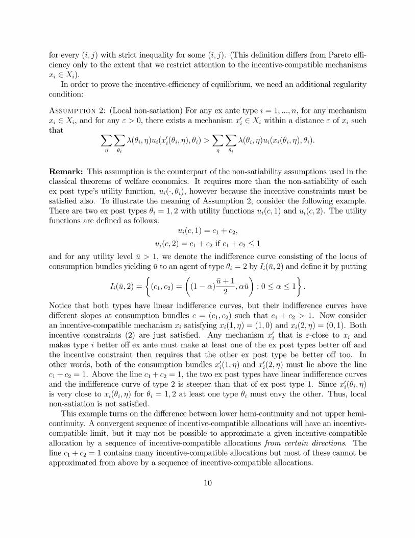
for every (i, j) with strict inequality for some (i, j). (This definition differs from Pareto effi-ciency only to the extent that we restrict attention to the incentive-compatible mechanismsxi ∈ Xi).In order to prove the incentive-efficiency of equilibrium, we need an additional regularity

condition:

Assumption 2: (Local non-satiation) For any ex ante type i = 1, ..., n, for any mechanismxi ∈ Xi, and for any ε > 0, there exists a mechanism x0i ∈ Xi within a distance ε of xi suchthat X

η

Xθi

λ(θi, η)ui(x0i(θi, η), θi) >

Xη

Xθi

λ(θi, η)ui(xi(θi, η), θi).

Remark: This assumption is the counterpart of the non-satiability assumptions used in theclassical theorems of welfare economics. It requires more than the non-satiability of eachex post type’s utility function, ui(·, θi), however because the incentive constraints must besatisfied also. To illustrate the meaning of Assumption 2, consider the following example.There are two ex post types θi = 1, 2 with utility functions ui(c, 1) and ui(c, 2). The utilityfunctions are defined as follows:

ui(c, 1) = c1 + c2,

ui(c, 2) = c1 + c2 if c1 + c2 ≤ 1and for any utility level u > 1, we denote the indifference curve consisting of the locus ofconsumption bundles yielding u to an agent of type θi = 2 by Ii(u, 2) and define it by putting

Ii(u, 2) =

½(c1, c2) =

µ(1− α)

u+ 1

2, αu

¶: 0 ≤ α ≤ 1

¾.

Notice that both types have linear indifference curves, but their indifference curves havedifferent slopes at consumption bundles c = (c1, c2) such that c1 + c2 > 1. Now consideran incentive-compatible mechanism xi satisfying xi(1, η) = (1, 0) and xi(2, η) = (0, 1). Bothincentive constraints (2) are just satisfied. Any mechanism x0i that is ε-close to xi andmakes type i better off ex ante must make at least one of the ex post types better off andthe incentive constraint then requires that the other ex post type be better off too. Inother words, both of the consumption bundles x0i(1, η) and x0i(2, η) must lie above the linec1+ c2 = 1. Above the line c1+ c2 = 1, the two ex post types have linear indifference curvesand the indifference curve of type 2 is steeper than that of ex post type 1. Since x0i(θi, η)is very close to xi(θi, η) for θi = 1, 2 at least one type θi must envy the other. Thus, localnon-satiation is not satisfied.This example turns on the difference between lower hemi-continuity and not upper hemi-

continuity. A convergent sequence of incentive-compatible allocations will have an incentive-compatible limit, but it may not be possible to approximate a given incentive-compatibleallocation by a sequence of incentive-compatible allocations from certain directions. Theline c1 + c2 = 1 contains many incentive-compatible allocations but most of these cannot beapproximated from above by a sequence of incentive-compatible allocations.

10

Theorem 2 Under the maintained assumptions, if (p, q, x, y) is an intermediated equilib-rium and Assumption 2 is satisfied, then the allocation (x, y) is incentive-efficient.

Proof. See Section 8.Theorem 2 is in the spirit of Prescott and Townsend (1984a, b), but the present model

takes the decentralization of the incentive-efficient allocation a step further. Markets areused in Prescott and Townsend (1984a, b) to allocate mechanisms to agents at the firstdate. After the first date all trade is intermediated by the mechanism. Here, markets arealso used for sharing risk and for intertemporal smoothing and intermediaries are activeparticipants in markets at each date. In Section 4 we show that efficiency requires thatindividuals do not have access to financial markets. To this extent, we follow Prescott-Townsend in assuming that individuals’ trade is intermediated by the mechanism. In Section5, we consider incomplete contracts and the possibility of default. In the event of default,individuals’ trade is no longer intermediated by the mechanism.Remark: An important qualification to the incentive-efficiency of the intermediated equi-librium is the “equilibrium selection” implicit in the definition of equilibrium. Followingthe standard principal-agent approach (see, e.g., Grossman and Hart (1983)), we allow theprincipal (the intermediary), to choose the actions of the agents (the investors), subject to anincentive-compatibility constraint. This assumption means that the intermediary can planwhat to do in each state. The complete markets can be used to ensure that liabilities canbe met in every state. As a result bankruptcy and financial crises cannot occur.Remark: The incentive-efficiency of equilibrium is in marked contrast to the results inBhattacharya and Gale (1987). The difference is explained by the informational assumptions.In the model above, there is no asymmetry of information in the markets for Arrow securities.Once the state η is observed, all aggregate uncertainty is resolved. The distribution of ex posttypes in each intermediary is a function of η and hence becomes common knowledge onceη is revealed. Trading Arrow securities at date 0 is sufficient to provide optimal insuranceagainst all aggregate shocks at date 1. In Bhattacharya and Gale (1987), by contrast, anintermediary’s true demand for liquidity is private information at date 1. Markets for Arrowsecurities cannot provide incentive-efficient insurance against private shocks.While symmetry of information in financial markets is a useful benchmark, one can

easily imagine circumstances in which intermediaries have private information, for example,the intermediary knows the distribution of ex post types among its depositors, but outsidersdo not. In that case, providing incentive-efficient insurance to the intermediaries wouldrequire us to supplement markets for Arrow securities with an incentive-compatible insurancemechanism, as in Bhattacharya and Gale (1987).

3.5 Examples

In this subsection we consider a series of numerical examples with complete markets andcomplete contracts with respect to aggregate states. These provide an efficient benchmarkfor subsequent examples with incomplete markets and/or contracts. We look first at anexample of asset-return shocks and then look at an example with liquidity shocks.

11

Return shocks

Example 1: We assume there is a single ex ante type of investor with Diamond-Dybvigpreferences. There are two ex post types, early consumers (θ = 1) and late consumers(θ = 2). The utility function is

u(c1, c2, θ) =

½log c1 θ = 1,log c2 θ = 2.

The probability of being an early consumer is one half, independently of the aggregate stateη. There are two equally likely aggregate states η = 1, 2 and the return on the long asset atdate 2 is contingent on the state:

R(1) = r;R(2) = 2.

Different equilibria are generated by varying r.Since investors are ex ante identical, the open interest in Arrow securities will be 0 in

equilibrium.Since the investors are either early or late consumers, the optimal bundles will be of the

form x(θ, η) = {(c1(η), 0), (0, c2(η))} with early consumers consuming c1(η) at date 1 andlate consumers consuming c2(η) at date 2. The market-clearing conditions are:

0.5c1(η) ≤ y (7)

0.5c1(η) + 0.5c2(η) = y + (1− y)R(η) (8)

for η = 1, 2.The form of the equilibrium depends on whether (7) is binding. In the first type of

equilibrium, it binds in both states; in the second, it only binds in state 2; in the third, itdoes not bind in either state.

Example 1A. For R(1) = r > 1, equilibrium is unique and 0.5c1(η) = y in both states.A typical equilibrium with r = 1.5 is shown in Table 1. The intermediary puts 0.5 in thesafe asset and 0.5 in the risky asset. The early consumers receive 1 at date 1 irrespective ofthe state, and late consumers receive 1.5 in state 1 and 2 in state 2. With these allocationsit is clear that the incentive constraint does not bind. No late consumer would choose 1at date 1 rather than 1.5 or 2 at date 2. The Arrow securities are priced at 0.5 for bothstates. The date 1 spot price of consumption is higher in state 1 than state 2 because date2 consumption is lower and marginal utility is higher in state 1.

Example 1B. For 0.4 ≤ r < 1, the unique pure intermediated equilibrium is such that theconsumption profile satisfies 0.5c1(1) < y and 0.5c1(2) = y. In state 1, the returns to thelong asset are so low that some of the short asset must be saved to provide consumption atdate 2; in state 2, all of the short asset is consumed at date 1. In order for the intermediariesto be willing to hold the short asset between date 1 and date 2 in state 1, the price must

12

be equal to 1. Thus, consumption is equalized across time in state 1. The amount investedin the short asset rises as the expected payoff on the long asset falls. Table 1 illustrates theequilibrium values for the case where r = 0.5. The amount invested in the safe asset hasmoved up to 0.64, in state 1 p2(1) = 1 and consumption is the same at both dates.

Example 1C. It remains to consider the case 0 ≤ r ≤ 0.4. As r continues to fall theintermediary invests more in the short asset and less in the long asset. The total output andconsumption in state 2 are also falling and for r < 0.4 the consumption at date 1 is less thanthe holding of the short asset in both states: 0.5c1(η) < y. Consumption is equalized acrosstime in both states. The equilibrium values corresponding to r = 0.3 are given in Table 1.Here y = 0.78, p1(1) = p2(1) = 1 and in both states consumptions are equated at each date.

The next example introduces a second ex ante type consisting of risk neutral investors.The purpose of this example is to illustrate how the Arrow securities allow cross-sectionalrisk sharing and to show their role in ensuring an incentive-efficient allocation.

Example 2. There are two ex ante types of investors, the risk averse investors, denoted byA,and the risk neutral investors denoted by N . The period utility functions are UA(c) = log(c)and UN(c) = c, respectively. The measure of each type is normalized to 1 and each type hasa probability 0.5 of being an early or late consumer. Otherwise things are the same as inExample 1.As in Example 1, the qualitative features of the equilibrium depend on whether some

of the short asset is carried over from date 1 to date 2. One case is sufficient to illustratehow the Arrow securities allow risk to be shared. For r ≥ 0.4 the allocation is the sameas in Example 1A, except that all uncertainty is absorbed by the risk neutral type. Theequilibrium portfolios are yA = 0.5 and yN = 0, for the representative intermediaries of typeA and type N, respectively.Table 1 gives the equilibrium values for the case where r = 0.5. The market-clearing

prices are q(1) = 0.5, q(2) = 0.5, p2(1) = 0.8, p2(2) = 0.8. The portfolio returns (receipts) ofeach intermediary and consumption of each type are given in the following table.

State 1 State 2(yA, R(η)(1− yA)) (0.5, 0.25) (0.5, 1)(yN , R(η)(1− yN)) (0, 0.5) (0, 2)(cA1(η), cA2(η)) (1, 1.25) (1, 1.25)(cN1(η), cN2(η)) (0, 0.25) (0, 4.75)

Risk sharing between the intermediaries for the two groups is achieved through trading inthe Arrow-security markets at date 0 and the spot consumption markets at date 1. In state1 the type A intermediaries have 0.5 of the good from their short asset holdings. They havepromised each of their 0.5 early consumers 1 unit of the good each so they can simply payout what they receive from the short asset to meet their obligations. At date 2 they receive0.25 from their holdings of the long asset. They have promised their 0.5 late consumers

13

1.25 each. The deficit is 0.5× 1.25− 0.25 = 0.375. To ensure that they have this they needto use the η = 1 Arrow security and the spot market at date 1. They purchase 0.3 units ofthe η = 1 Arrow security at date 0 for q(1) × 0.3 = 0.5 × 0.3 = 0.15 and then use the 0.3they receive at date 1 in state 1 to purchase 0.3/p2(1) = 0.3/0.8 = 0.375 of the date 2 goodin the date 1 spot market. At date 0 they finance the 0.15 needed to purchase the η = 1Arrow security by selling 0.375 of the good at date 2 in state 2 and 0.3 of the η = 2 Arrowsecurity. Since they have 1 unit of output from their long asset at date 2 this will leave themwith 0.625 of the good to pay out to their 0.5 late consumers who receive 1.25 each. Thetype N ’s are willing to take the other side of these trades since they are risk neutral. It canbe seen that this improvement in risk sharing increases the expected utility of type A’s from0.054 in Example 1B to 0.112 here.There are other intermediated equilibria corresponding to these parameter values. In

particular, the portfolio holdings of the type-A intermediaries are not uniquely determined.For example, the type-A intermediaries could hold less of the short term asset and moreof the long term asset, as long as this is offset by changes in the holdings of the type-Nintermediaries. As long as the aggregate portfolio remains the same, investors’ consumptionand welfare is unchanged.

Liquidity shocks

The uncertainty in Examples 1 and 2 is generated by shocks to asset returns. Similar resultscan be obtained by assuming aggregate uncertainty about the demand for liquidity.

Example 3. This example is similar to Example 1. There are two main differences. First,it is assumed that there is no uncertainty about the return to the long asset:

R(1) = R(2) = r.

Second, there is aggregate uncertainty about the demand for liquidity. The states η = 1, 2are equally likely but now the proportions of early and late consumers differ across states:

Proportion State 1 State 2Early consumers 0.4 0.6Late consumers 0.6 0.4

By varying r we can generate the same phenomena as in the case of return shocks. Ratherthan go through all the different cases, we illustrate a pure intermediated equilibrium forthe case r = 1.6. The equilibrium values are shown in Table 1. For this case the aggregateliquidity constraint binds in both states because the return on the long asset is high. Atdate 1 all the proceeds from the short asset are used for consumption. In state 1 aggregateliquidity needs are low at date 1. Since consumption is split evenly among early consumersper capita consumption is high compared to state 2 where aggregate liquidity needs are highat date 1. At date 2 there are many late consumers in state 1 so consumption per capita islower than in state 2 where there are relatively few late consumers.

14

4 Complete participation and redundancy

Cone (1983) and Jacklin (1986) have pointed out that the beneficial effects of banks in theDiamond-Dybvig (1983) model depend on the assumption individuals are not allowed totrade assets at the intermediate date. Increasing access to financial markets actually lowerswelfare. If investors are allowed to participate in asset markets, then the market allocationweakly dominates the allocation implemented by the banks.In this section, we show that with complete markets and complete market participation,

banks are redundant in the sense that they cannot improve on the risk sharing achieved bymarkets alone. The ability of intermediaries to provide insurance against shocks to liquiditypreference depends crucially on the assumption that investors cannot participate directly inasset markets. To show this, we first characterize an equilibrium with markets but withoutintermediaries. Then we show that the introduction of intermediaries is redundant.The market data is the same as in Section 2. Investors are allowed to trade in markets

for Arrow securities at date 0 and can trade in the spot markets for the good at date 1. Letyi denote the portfolio chosen by a representative investor of type i and let xi(θi, η) denotethe consumption bundle chosen by an investor of type θi in state η. The investor’s choice of(xi,yi) must solve the decision problem:

maxP

η

Pθiλ(θi, η)ui(xi(θi, η), θi)

s.t.P

η q(η) · xi(θi, η) ≤P

η q(η)p(η) · (yi, (1− yi)R(η)),∀θi.

The maximization problem for the individual is similar to that of an intermediary of typei except for two things. First, there is no explicit incentive constraint xi ∈ Xi. Second,there is no insurance provided against the realization of θi. This is reflected in the fact that,instead of summing the budget constraint over η and θi, it is summed over η only and mustbe satisfied for each θi. The ex ante type i can redistribute wealth across states η in any wayhe likes, but each type θi will get the same amount to spend in state η. As a result, for eachrealization of θi in a given state η, the choice of xi(θi, η) must maximize the utility functionui(xi(θi, η), θi) subject to a budget constraint that depends on η but not on θi. This ensuresthat incentive compatibility is satisfied.An equilibrium for this economy consists of a price system {p, q} and an attainable

allocation {(xi, yi)} such, that for every type i, (xi, yi) solves the individual investor’s problemabove.Comparing this definition of equilibrium with the intermediary equilibrium, it is clear

that an equilibrium with complete market participation cannot implement the incentive-efficient equilibrium except in the special case where there are no gains from sharing riskagainst liquidity preference shocks.The more interesting question is whether introducing intermediaries in this context can

make investors any better off. The answer, as we have suggested, is negative. To see this,note first of all that in an equilibrium with complete participation, all that investors careabout in each state is the market value of the bundle they receive from the intermediary. Ifan intermediary offers a mechanism xi the investors of type θi will report the ex post type θi

15

that maximizes p(η) · xi(θi, η) in state η. Using the Revelation Principle, there is no loss ofgenerality in assuming that the value of consumption p(η) · xi(θi, η) = wi(η) is independentof θi. But this means that the intermediary can do nothing more than replicate the effect ofthe markets for Arrow securities. More precisely, the intermediary is offering a security thatpays wi(η) in state η and the intermediary’s budget constraintX

η

q(η)wi(η) ≤Xη

q(η)p(η) · (yi, (µi − yi)R(η))

ensures that {wi(η)} can be reproduced as a portfolio of Arrow securities at the same cost.Theorem 3 In an equilibrium with complete market participation, the introduction of in-termediaries is redundant in the sense that an equilibrium allocation in an economy withintermediaries is payoff-equivalent to (i.e., yields the same expected utilities as) an equilib-rium allocation of the corresponding economy without intermediaries.

This is, essentially, a “Modigliani-Miller” result, saying that whatever an intermediary cando can be done (and undone) by individuals trading on their own in the financial markets.This result underlines the role of assuming incomplete participation. Given gains fromsharing the risk of liquidity shocks that intermediaries provide, complete participation isundesirable.Theorem 2 provides conditions under which an equilibrium will be incentive-efficient.

However, the equilibrium described in Theorem 2 does not necessarily Pareto-dominate theequilibrium described in Theorem 3: with many ex ante types, it is possible that one typei will be worse off in the incentive-efficient equilibrium. In the special case where there is asingle ex ante type, complete participation makes everyone worse off. The results of Cone(1983) and Jacklin (1986) referred to earlier assume a single ex ante type of investor.

5 Incomplete contracts and default

In the benchmarkmodel defined in Section 3, intermediaries use general, incentive-compatiblecontracts. In reality, we do not observe such complex contracts. There are many reasons forthis which are well documented in the literature. These include transaction costs, asymmet-ric information and the nature of the legal system. These kinds of assumption can justify theuse of debt and many other kinds of contracts that intermediaries use in practice. Since weare interested in developing a general framework we do not model any specific justificationfor incomplete contracts. Instead we assume that the contract incompleteness can take anyform and prove results that hold for any type of incomplete contract.With complete contracts, intermediaries can always meet their commitments. Default

cannot occur. Once contracts are constrained to be incomplete, then it may be optimalfor the intermediary to default in some states. In the event of default, it is assumed thatthe intermediary’s assets, including the Arrow securities it holds, are liquidated and theproceeds distributed among the intermediary’s investors. For markets to be complete, which

16

is an assumption we maintain for the moment, the Arrow securities that the bank issuesmust be default free. Hence, we assume that these securities are collateralized and theirholders have priority. Anything that is left after the Arrow securityholders have been paidoff is paid out pro rata to the depositors.An intermediary of type i chooses a formal contract xi ∈ XI

i and an indicator functionB : H → {0, 1}, whereB(η) = 1means that the intermediary defaults on the formal contract.There is also a ‘default contract’, which describes what happens when the intermediarydefaults. The ‘default contract’ xi is defined by x (θi, η) = (wi(η), 0), where wi(η) is theliquidated value of assets in state η. The ‘default contract’ is not part of the formal contract;it is determined by the institution of bankruptcy (the nexus of law, courts, creditors anddebtors) when the contract has been breached. Formally, it is possible to describe all this asa single mechanism, which is what we do, but conceptually there is an important differencebetween what the formal contract says and what happens if the formal contract is breached.The institution of bankruptcy is exogenous to the model, something the intermediary takesas given when writing the contract.Given this bankruptcy procedure, an intermediary has to choose two contracts for individ-

uals, a formal contract xi ∈ XIi and a default contract xi, and a decision rule B : H → {0, 1}

that indicates when the bank defaults. Then the effective contract xi is defined by

(1−B(η))xi(θi, η) +B(η)xi(θi, η)

for every (θi, η). Since everything is paid out at date 1 in the event of default, investors usethe short asset to provide consumption at date 2. Then the utility of a contract xi generatedin this way is given by u∗i (xi(θi, η), θi) in the state (θi,η) and the incentive constraint is

u∗i (xi(θi, η), θi) ≥ u∗i (xi(θi, η), θi),∀θi, θi ∈ Θi.

Let Xi denote the set of incentive-compatible contracts generated in this way.To demonstrate how default works consider the following simple illustration.

Example Suppose that intermediaries are restricted to offering non-contingent contracts.Then xi ∈ XI if and only if

xi(θi, η) = xi(θi, η0)

for any η, η0 ∈ H. If we assumed further that agents were either early consumers, who valueconsumption at date 1, or late consumers who value consumption at date 2, we could withoutloss of generality write the contract as

xi(θi, η) =

½(c1, 0) if θi = 0(0, c2) if θi = 1.

This contract is highly inflexible because it does not allow the intermediary to adjust thepayment across states in response to changing demands for liquidity or changing asset re-turns. If default is not allowed, the intermediary is forced to distort the contract. Default

17

allows the intermediary to replace this inflexible contract with the following:

xi(θi, η) =

(c1, 0) if θi = 0, Bi(η) = 0,(0, c2) if θi = 1, Bi(η) = 0,(wi(η), 0) if Bi(η) = 1.

The possibility of incomplete contracts is represented by restricting the choice of contractto a subset Xi ⊂ Xi. The theory developed in Section 3 is essentially the same, but withXi replaced by Xi. With this substitution, an intermediated equilibrium becomes an inter-mediated equilibrium with incomplete contracts, an incentive-efficient allocation becomes aconstrained-efficient equilibrium, and Assumption 2 becomes Assumption 20. Then Theorem2 can be interpreted as a theorem about constrained-efficiency of equilibrium with incompletecontracts but complete markets.

Theorem 4 Under the maintained assumptions, if (p, q, x, y) is an intermediated equilib-rium with incomplete contracts and Assumption 20 is satisfied, then the allocation (x, y) isconstrained-efficient.

Although this result is a direct corollary of Theorem 2, it is substantively the mostimportant result of the paper, for it shows that, in the presence of complete markets, theincidence of default is optimal in a laisser-faire equlibrium. For example, consider the casewhere banks are restricted to using demand deposits that promise a fixed payment at date1. A bank may default in some states because its assets are insufficient to meet its non-contingent commitments. Default allows the bank to make its risk-sharing contract morecontingent, i.e., more complete. But if several banks default in the same state, this maycause a financial crisis, as the simultaneous liquidation of several banks forces down assetprices, which may in turn cause distress in other banks. Nonetheless, the theorem shows that,given complete markets for insuring against aggregate shocks, the occurence of these crisesis optimal and not a market failure. There is no scope for welfare-improving governmentintervention to prevent financial crises.Remark: The definition of constrained efficiency is formally similar to the definition ofincentive-efficiency–we simply substitute X for X in the latter–but there are importantsubstantive differences. The definition of X implicitly incorporates the “bankruptcy code”and requires consumers to be autarkic once the intermediary defaults. Allowing trade afterdefault would complicate the theory but should not change the basic result as long as marketsfor aggregate risk are incomplete.Remark: Alonso (1996) and Allen and Gale (1998) have argued that financial crises cansometimes be optimal, or at least Pareto-preferred to government intervention to suppresscrises entirely. While these arguments have a similar flavor to the present results, they aresubstantially different. Both Alonso (1996) and Allen and Gale (1998) rely on very specialexamples to show that laisser faire may be preferred to a policy of preventing financial crises.There is no general efficiency result. In fact, Allen and Gale (1998) show that even withinthe context of their example, the efficiency of financial crises is not robust.

18

More importantly, there is no role for Arrow securities in the examples provided byAlonso (1996) and Allen and Gale (1998). In their models, a representative bank chooses aportfolio and deposit contract to maximize the expected utility of the representative agent.Because of the representative agent assumption, banks are autarkic and complete marketsare irrelevant. So the results presented here are based on a different argument and apply toa much broader class of economies.Remark: The role of Arrow securities deserves further attention in a model with default.An Arrow security is a promise to deliver one unit of the good in some state at date 1.It is assumed, crucially, that Arrow securities are fully collateralized so there is no risk ofdefault on these promises. Equivalently, traders in Arrow securities can anticipate eachintermediary’s ability to repay borrowing through Arrow securities in each state and Arrowsecurities take priority over other claims on the intermediary’s assets. This means that, atdate 0, the intermediary will not be allowed to execute trades that cannot be fulfilled at date1 and that the intermediary’s position in Arrow securities is settled at the beginning of date1 before anything else happens, in particular, before the default decision is made and beforeinvestors receive any payments. These assumptions are restrictive but they are essential tothe definition of Arrow security markets.Remark: Default is completely voluntary in the sense that the intermediary chooses atdate 0 those states in which it wishes to default. Default is not forced on the intermediaryby the budget constraint, in fact, in the presence of complete markets it is not clear whatthis would mean. Because Arrow security markets are complete, there is a single budgetconstraint and the intermediary chooses the amount of wealth allocated to each state. Wedo however assume that the intermediary is committed to his default decision at date 0and further, that he makes the default decision in the ex ante interest of the representativeinvestor. These assumptions are restrictive but interesting insofar as they are required forefficiency. We can interpret them as a description of an optimal bankruptcy institution.

5.1 Examples

In this section we demonstrate a number of results using examples. These results includethe following.

1. The existence (indeed necessity) of mixed equilibria.

2. The optimality of default and crises.

3. Cash-in-the-market pricing when there is a crisis.

4. Suboptimal risk sharing with incomplete markets.

There are many examples of intermediaries that use incomplete contracts with theirdepositors. As we have seen, as soon as incomplete contracts are introduced the possibilityof default must be allowed for. This in turn introduces the possibility of financial crises. Inpractice crises can be precipitated by a wide array of intermediaries. Historically, however, it

19

has been banks that have caused most crises. In order to illustrate the model with incompletecontracts and default we consider examples where the intermediaries are banks, that is, theyare restricted to issuing deposit contracts. A deposit contract promises a fixed payment atdate 1. If the bank is unable to meet its commitment to its depositors, then it is liquidatedand all its assets are sold. If it can meet its commitment depositors can keep their funds inthe bank until date 2.

Example 4. To illustrate the properties of a banking equilibrium, we revert to the param-eters from Example 1.

Example 4A. For r ≥ 1 the first best can again be implemented as a banking equilibrium.The first-best allocation requires that consumption at date 1 be the same in both states, sothe optimal incentive-compatible contract is in fact a deposit contract. Moreover, bankruptcydoes not occur in equilibrium. The allocation corresponding to a pure banking equilibrium isexactly the same as the allocation corresponding to a pure intermediated equilibrium, whichas we have seen is the same as the first best. For r = 1.5, for example, the equilibrium valueswill be the same as for Example 1A, as shown in Table 1.The main difference between Examples 1A and 4A is that the prices supporting the

first best allocation are unique in Example 1A but are not in Example 4A. In Example 1Athe general intermediaries can freely vary payoffs across states and dates so only one set ofprices can support the optimal allocation. Because the banks are restricted to using depositcontracts in Example 4A, consumption at date 1 is independent of the state as long as thereis no bankruptcy. This prevents the banks from arbitraging between the states at date 1. Ineffect, we have lost one equilibrium condition compared with the intermediated equilibrium.Any vector of prices (q(1), q(2), p2(1), p2(2)) that supports the equilibrium allocation at date2 is consistent with a banking equilibrium. The following no-arbitrage conditions are satisfied

q(1)p2(1) = 0.33 (9)

q(2)p2(2) = 0.25 (10)

q(1) + q(2) = 1 (11)

and the existence of the short asset implies that

p2(1) ≤ 1; p2(2) ≤ 1.Combining these conditions, it follows that the range of possible prices for q(1) is

0.33 ≤ q(1) ≤ 0.75.The other prices are determined by (9)-(11).For r < 1 deposit contracts cannot be used to implement the first best or incentive-

efficient allocation. In particular, a deposit contract that is consistent with the incentive-efficient consumption in state 2 would imply bankruptcy in state 1 (see, e.g., Example 1B).If all banks were to offer a contract which allowed bankruptcy in state 1 they would all be

20

forced to liquidate their assets. If they all do this, there is no bank on the other side of themarket to buy the assets and the price of future consumption, p2(1), falls to 0. This cannotbe an equilibrium because it would be worthwhile for an individual bank to offer a contractwhich did not involve bankruptcy. This bank could then buy up all the long term asset instate 1 at date 1 for p2(1) = 0 and make a large profit.This argument indicates that for r < 1 there cannot be a pure banking equilibrium

with bankruptcy. There are two other possibilities. One is that there is a pure equilibriumin which all banks remain solvent. The other is that there is a mixed equilibrium in whichbanks choose different contracts and portfolios. In particular, a group of banks with measureρ makes choices that allow it to remain solvent in state 1 while the remaining 1 − ρ banksgo bankrupt. The banks that are ensured of solvency are denoted type S while those thatcan go bankrupt are denoted type B. It turns out that both the pure equilibrium with allbanks remaining solvent and the mixed equilibrium can occur when r < 1.

Example 4B. For 0.90 ≤ r < 1 there is a pure banking equilibrium in which all the bankschoose to remain solvent (ρ = 1). There is again a range of prices which can support theallocation. Type-S banks stay solvent by lowering the amount promised at date 1, loweringtheir investment in the short asset and increasing their investment in the long asset. Theequilibrium values for the case where r = 0.95 are shown in Table 1. The range of q(1) thatwill support the allocation and prevent entry by type B banks is 0.55 < q(1) < 0.77. Theother prices are determined by the equilibrium conditions

q(1)p2(1) = 0.54

q(2)p2(2) = 0.24

q(1) + q(2) = 1.

Example 4C. For 0 < r < 0.90 there exists a mixed banking equilibrium. At the boundaryr = 0.90, the set of prices that will support the equilibrium of the type shown in Example 4Bshrinks to a singleton: (q(1) = 2/3, q(2) = 1/3). For values of r < 0.90 but close to 0.90 theproportion of type-S banks is large (ρ ≈ 1). As r falls, the proportion of type-B banks risesuntil as r goes to 0 the proportion of type-B banks 1− ρ approaches 1. The mixed bankingequilibrium corresponding to r = 0.5 is shown in Table 1. The proportion of type-S banksis ρ = 0.35. As in the earlier examples, the portfolios of individual banks are indeterminate.It is only the aggregate portfolio that is determined by the equilibrium conditions.The pricing of assets in state 1 in Example 4C illustrates the principle of “cash-in-the-

market pricing”. When the type-B banks go bankrupt in state 1 they have to liquidate alltheir holdings of the long asset. These are purchased by the type-S banks who use all oftheir spare liquidity to do so. In making the decision on how much of the short asset to holdthey trade off the benefits of liquidity in the low output state with the cost of holding idlefunds in the high output state.

21

The effect of cash-in-the-market pricing can be seen if we compare this example withExample 1B. The price of the long asset is 0.5× 1 = 0.5 in Example 1B and 0.5× 0.9 = 0.45in the present example. It can easily be shown that the price of the long asset could bedepressed further by changing the parameters. For example, the lower the probability of thelow-output state, the less liquidity the type-S bank will hold and the lower the price of thelong asset will be in the low-output state.The mixed equilibrium in Example 4C illustrates a number of interesting phenomena.

First, banks serving identical depositors may do quite different things in equilibrium. Onesubset will find it optimal to follow a safe strategy and avoid the risk of bankruptcy. Anothersubset will follow a risky strategy that makes bankruptcy inevitable in state 1. As a result,even when all investors are identical ex ante, there can be a financial crisis in which somebanks remain solvent while others go under. In the context of the example, the crisis is moresevere when the state-1 return r is lower. However, the results in Section 5 show that thesecrises are consistent with the constrained efficiency of equilibrium. There is no justificationfor intervention or regulation of the financial system. A planner could not do better.Many analyses of banking assume that there is a technology for early liquidation of the

long term asset. The resulting equilibria are typically symmetric. This example illustratesthat this assumption materially changes the form of the equilibrium. With endogenousliquidation one group of banks must provide liquidity to the market and this results inmixed equilibria.A comparison of Example 4C with Example 1 shows the importance of non-contingent

contracts in causing financial crises. In Example 1 the ability to use state contingent contractswith investors means that bankruptcy never occurs and as a result there is never a crisis.However, with deposit contracts crises of varying severity always occur in the low outputstate.There are a number of other types of equilibrium, depending on whether the short asset

is held between date 1 and date 2 and the number of ex ante groups. The properties of theseequilibria are similar to those illustrated in Examples 1 and 2 and will not be repeated here.In Example 4 it was assumed that markets are complete. However, it can straightfor-

wardly be seen that with incomplete markets the allocation in each case would be the same.In Examples 4A and 4B there is only one ex ante type in equilibrium and they all do the samething so the open interest in Arrow securities is zero and there is no role for risk sharing.In the mixed equilibrium of Example 4C there are two types of banks providing differentallocations even though ex ante all investors are identical. Complete markets do not helprisk sharing, however. The reason is that the contract forms restrict the amounts that canbe paid out and the trade-offs given these mean that no improvement can be made. Theonly difference in Example 4C if markets are incomplete is the equilibrium holdings of assetsof the two banks are now unique. The type-S banks hold 0.82 of the short asset and thetype-B banks hold 0.59 of it. This fact that complete markets does not make a differencehere is clearly a special case as the next example, which mixes Example 2 and Example 4C,demonstrates.

22

Example 5A. The example is the same as Example 2 except that contracts are incomplete.There are risk averse type-A investors and risk neutral type-N investors, r = 0.5 and thereare complete Arrow security markets. It can straightforwardly be seen that the equilibriumis exactly the same as that shown in Table 1 for Example 2. The type-A banks can use adeposit contract promising 1 at date 1 to implement the optimal allocation. Similarly thetype-N banks can use a deposit contract promising 0 at date 1.

Example 5B. This example is the same as Example 5A except now there are no Arrowsecurities so markets are incomplete. Here it can be seen that the equilibrium is essentiallythe same as in Example 4C. The banks for the type-A investors behave exactly as in Example4C. The banks for the type-N investors do not find it worthwhile to enter the markets thatdo exist. They simply put all their customers endowment in the long asset and pay out 0 atdate 1 and whatever is produced at date 2.

A comparison of Examples 5A and 5B demonstrates the crucial role that complete mar-kets can play. With complete markets the financial system produces the first best allocation.However, with incomplete markets the allocation is much worse. Moreover the incomplete-ness of markets leads to default and crises in equilibrium.In conclusion, the examples in this section have demonstrated the results mentioned

initially. First, Example 4C has shown that a mixed equilibrium can exist. When thereis only one type of bank they cannot all go bankrupt at the same time. If they did therewould be nobody to buy their assets and the assets’ price would fall to 0. This cannot bean equilibrium though since it would be worthwhile for a bank to stay solvent and buy upall the assets at the 0 price. As a result the equilibrium must be mixed.Second, Example 4C shows that default can be optimal for the banks. Theorem 4 shows

that the crises that result from banks’ defaulting are also socially optimal. In fact crises arenecessary for the constrained-efficient allocation to be achieved.Third, the logic demonstrating the existence of mixed equilibria shows how cash-in-the-

market pricing occurs. In making their decision on how much of the short asset to hold, thesolvent banks take into account the fact that if there is a crisis they can buy up the longasset cheaply and trade this off against the cost of not investing in the long asset at date 0and rolling over the liquidity in state 2.Fourth, Example 5 demonstrates the important role of complete markets. With incom-

plete markets the equilibrium is completely different from the one with complete markets.Not only is risk sharing much better with complete markets but also there are no crises.

6 Incomplete markets and liquidity regulation

The absence of markets for insuring individual liquidity shocks does not by itself lead tomarket failure. As we showed in Section 3, intermediaries with complete contracts canachieve an incentive-efficient allocation of risk under certain conditions. We showed inSection 5, under the same conditions, that intermediaries with incomplete contracts can

23

achieve a constrained-efficient allocation of risk. Two assumptions are crucial for theseresults: markets for aggregate uncertainty are complete (there is an Arrow security for eachstate η) and market participation is limited. Markets for aggregate risk allow intermediariesto share risk among different ex ante types of investor and limited participation allowsintermediaries to offer insurance against the realization of ex post types.In order to generate a market failure and provide some role for government intervention,

an additional friction must be introduced. Here we assume that it comes in the form ofincomplete markets for aggregate risk. There are two sources of aggregate risk in this model.One is the return to the risky asset R(η); the other is the distribution of investors’ liquiditypreferences λ(θi, η). Although there is a continuum of investors, correlated liquidity shocksgive rise to aggregate fluctuations in the demand for liquidity.Market incompleteness may be expected to vary according to the source of the risk.

On the one hand, asset returns can be hedged using markets for stock and interest rateoptions and futures. For example, financial markets allow intermediaries to take hedgingpositions on future asset prices and interest rates. Additional hedges can be synthesizedusing dynamic trading strategies. On the other hand, liquidity shocks seem harder to hedge.Asset prices and interest rates are functions of the aggregate distribution of liquidity shocksin the economy. Inverting this relationship, we can use asset prices and interest rates to inferthe average demand for liquidity, but not the liquidity shock experienced by a particularintermediary. Hence, trading options and futures will not allow intermediaries to provideinsurance against their own liquidity shocks. So markets for hedging liquidity shocks arelikely to be more incomplete than the markets for hedging asset returns.We analyze a polar case below: we assume that there exist complete markets for hedging

asset return shocks, but no markets for hedging liquidity shocks. Since complete markets forasset-return shocks permit efficient sharing of that risk, we might as well assume that assetreturns are non-stochastic. In what follows, we adopt the simplifying assumption that thereturn to the long asset is a constant r > 1 and the only aggregate uncertainty comes fromliquidity shocks.We continue to assume that each intermediary serves a single type of investor. Let xi

denote the mechanism and yi the portfolio chosen by the representative intermediary of typei. The problem faced by the intermediary is to choose (xi, yi) to maximize the expected utilityof the representative depositor subject to multiple, state-contingent budget constraints:

maxP

η

Pθiλ(θi, η)ui(xi(θi, η), θi)

s.t. xi ∈ Xi;Pθiλ(θi, η)p(η) · xi(θi, η)

≤ p(η) · (yi, (µi − yi)R(η)),∀η.The incompleteness of markets is reflected in the fact that there is a separate budget con-straint for each aggregate state of nature η, rather than a single budget constraint thatintegrates surpluses and deficits across all states.With incomplete markets, the existence of welfare-improving interventions is well known

in many contexts (cf. Geanakoplos and Polemarchakis (1986)). Rather than pursuing general

24

inefficiency results, we investigate a more specific policy intervention: Is there too much ortoo little liquidity in a laisser-faire equilibrium? The interest of the results follows not fromthe existence of a policy that increases welfare, but rather from the precise characterizationof the optimal (small) intervention to regulate liquidity. Our intuition suggests that marketprovision of liquidity will be too low when markets are incomplete. However, even in anequilibrium with a lot of structure, our analysis shows that whether there is too much or toolittle liquidity depends crucially on the degree of relative risk aversion.We identify liquidity regulation with manipulation of portfolio choices at the first date.

For example, a lower bound on the amount of the short asset held by intermediaries can beinterpreted as a reserve requirement. We examine regulation in the context of an economywith Diamond-Dybvig preferences.As usual, there are n ex ante types of investors i = 1, ..., n. The ex ante types are

symmetric and the size of each type is normalized to µi = 1. There are two ex post types,called early consumers and late consumers. Early consumers only value consumption at date1, while late consumers only value consumption at date 2. The ex ante utility function oftype i is defined by

ui(c1, c2, θi) = (1− θi)U(c1) + θiU(c2),

where θi ∈ {0, 1}. The period utility function U : R+→ R is twice continuously differentiableand satisfies the usual neoclassical properties, U 0(c) > 0, U 00(c) < 0, and limc&0 U 0(c) =∞.Each intermediary is characterized at date 1 by the proportions of early and late con-

sumers among its customers. Call these proportions the intermediary’s type. Then aggregaterisk is characterized by the distribution of types of intermediary at date 1. We assume thatthe cross-sectional distribution of types is constant and no variation in the total demand forliquidity. In this sense there is no aggregate uncertainty. However, individual intermediariesreceive different liquidity shocks: some intermediaries will have high demand for liquidityand some will have low demand for liquidity. The asset market is used to re-allocate liquidityfrom intermediaries with a surplus of liquidity to intermediaries with a deficit of liquidity. Itis only the cross-sectional distribution of liquidity shocks that does not vary. To make thisprecise, we need additional notation. We identify the state η with the n-tuple (η1, ..., ηn),where ηi is the fraction of investors of type i who are early consumers in state η. The fractionof early consumers takes a finite number of values, denoted by 0 < σk < 1, where k = 1, ..., K.We assume that the marginal distribution of ηi is the same for every type i and that thecross-sectional distribution is the same for every state η. Formally, let λk denote the ex anteprobability that the proportion of early consumers is σk. Let Hik = {η ∈ H : ηi = σk}.Then λk =

Pη∈Hik

λi(0, η), for every k and every type i. Ex post, λk equals the fraction ofex ante types with a proportion σk of early consumers. Then λk = n−1#{i : ηi = σk}, forevery k and every state η.The return on the long asset is non-stochastic,

R(η) = r > 1,∀η.The only aggregate uncertainty in the model relates to the distribution of liquidity shocksacross the different ex ante types i.

25

In what follows, we focus on symmetric equilibrium, in which the prices at dates 1 and2 are independent of the realized state η and the choices of the intermediaries at date 0 areindependent of the ex ante type i. Let the good at date 1 be the numeraire and let p denotethe price of the good at date 2 in terms of the good at date 1. At date 0 the representativeintermediary of type i chooses a portfolio yi = y and a consumption mechanism xi(η) = x(ηi)to solve the following problem:

maxP

k λk {σkU(x1(σk)) + (1− σk)U(x2(σk))}s.t. σkx1(σk) + (1− σk)px2(σk) ≤ y + pr(1− y), ∀k,

x1(σk) ≤ x2(σk),∀k.(12)

The incentive constraint x1(σk) ≤ x2(σk) is never binding. To see this, drop the incen-tive constraint and solve the relaxed problem. The special early-consumer, late-consumerstructure of preferences and the assumption r > 1 imply that the incentive constraint isautomatically satisfied by the solution to the relaxed problem.A symmetric equilibrium consists of an array (p, x, y) such that (x, y) solves the problem

(12) for the equilibrium price p and the market-clearing conditionsPKk=1 λkσkx1(σk) ≤ y,PKk=1 λk {σkx1(σk) + (1− σk)x2(σk)} = y + r(1− y).

are satisfied.To study the effect of regulation of intermediaries, we take as given the choice of portfolio

y at date 0 and consider the determination of the consumption mechanism x and the market-clearing price p. Call (p, x, y) a regulated equilibrium if x solves the problem (12) for thegiven values of p and y, and (x, y) satisfies the market-clearing conditions (15).Suppose that (p, x, y) is a regulated equilibrium and p > p∗. Then the short asset is

dominated by the long asset between dates 0 and 1 and no one will want to hold the shortasset. If the regulator requires intermediaries to hold a minimum amount of the short assetthen each intermediary will want to hold the minimum. In that case, (x, y) solves themaximization problem (12) subject to the additional constraint y ≥ y for an appropriatelychosen value of y. Similarly, if p < p∗ then the long asset is dominated and (x, y) solvesthe maximization problem subject to an additional constraint y ≤ y. Thus, any regulatedequilibrium can be interpreted as an equilibrium in which the intermediaries choose themechanism x and the portfolio y to maximize the expected utility of the depositors subjectto a constraint that requires them to hold a minimum amount of the short asset in the casep > p∗ or of the long asset in the case p < p∗. In this sense, the regulator can implement theregulated equilibrium (p, x, y) by imposing an appropriate constraint y on the intermediaries’portfolio choice.By manipulating the intermediaries’ portfolio choice, the regulator is able to manipulate

the equilibrium price p. The welfare effect of this change in price depends on the degree ofrisk aversion. We can state a positive result for regulatory policy as follows: it is possible toincrease welfare by imposing a lower bound on intermediaries’ holdings of the short asset if

26

the degree of relative risk aversion is greater than one. More precisely, let W (p) denote theexpected utility of the typical depositor in the regulated equilibrium (p, x, y).

Theorem 5 If (p∗, x∗, y∗) is a symmetric equilibrium and −U 00(c)c/U 0(c) > 1, then for somey > y∗ there is a regulated equilibrium (p, x, y) in which intermediaries are required to holdat least y units of the short asset and W (p) > W (p∗).

The proof of this result is in Section 8. The key step in the argument is provided by thefollowing lemma, which shows how the degree of risk aversion determines the welfare effectof a change in the regulated equilibrium price.

Lemma 6 For any p > p∗ sufficiently close to p∗, W (p) > W (p∗) if

−U00(c)cU 0(c)

> 1. (13)

For any p < p∗ sufficiently close to p∗, W (p) > W (p∗) if

−U00(c)cU 0(c)

< 1.

Proof. See Section 8.So an increase in liquidity (increase in the price of the long asset) may increase or decreasewelfare, depending on the degree of risk aversion.The intuition behind this result is the following. When relative risk aversion is high,

optimal risk sharing requires that consumption at date 1 is higher than the present value ofconsumption at date 2, that is, c1 > pc2. An increase in the fraction of early consumers σ,cet. par., implies an increase in the present value of total consumption σc1 + (1− σ)pc2. Inorder to satisfy the budget constraint,

σc1 + (1− σ)pc2 = y + pr(1− y),

both c1 and c2 must fall (efficient risk-sharing implies that c1 and c2 always rise and falltogether). Then (1− σ)c2, the total consumption at date 2, falls and the budget constraintimplies that σc1, the total demand for liquidity at date 1, rises. So per capita consumptionat dates 1 and 2 and demand for liquidity go in opposite directions. From this it follows that,when σ is high, σc1 > y and (1−σ)c2 < r(1−y), so an increase increase in liquidity (increasein p), has a positive income effect and raises consumption and, when σ is low, an increasein liquidity has the opposite effect. Thus, an increase in liquidity lowers consumption ingood states (where per capita consumption is high) and raises it in bad states (where percapita consumption is low). This transfer from high-consumption states to low-consumptionstates raises welfare. When relative risk aversion is low, the argument works in the oppositedirection. The welfare effect depends on the correlation between equilibrium consumptionand the liquidity shocks.

27

7 Concluding Remarks

We have argued that, contrary to the conventional wisdom, it is not axiomatic that financialcrises are bad from a welfare point of view. In fact, we have presented conditions under whichthey are essential for constrained efficiency. This should give economists pause for thought.Although the conditions for efficiency are restrictive, they are no more so than the conditionsusually required for efficiency of general equilibrium. We should also note that, while thefocus of this paper is on a rudimentary model of banks and financial intermediaries, the basicideas have a wider application. Wherever incompletely contingent contracts, such as debtcontracts, are used, there is the possibility of default. In the absence of complete markets forthe aggregate risks involved, financial crises in the form of widespread default may constitutea market failure requiring some form of intervention by the financial regulator.The model we have used is special in several respects. For example, we have assumed

that investors are condemned to autarky after a default. A more realistic model wouldallow intermediaries to enter and offer deposit contracts to investors whose intermediarieshave defaulted at date 1. We have seen, in Section 4, that incentive-efficient risk sharingrequires limited participation in markets. In particular, we cannot allow investors to dealwith more than one bank at a time. If investors could deal with a second bank ex post, thiscould undermine the incentive constraints in the original contract and result in lower welfare.However, once an intermediary has defaulted, there is no reason to prevent investors fromaccepting contracts with the surviving intermediaries and thus avoiding the inefficiency thatarises from being excluded from asset markets. This would be more complicated, but wouldnot fundamentally alter the results, as long as entry occurs after the original intermediaryhas defaulted and liquidated its assets.Although we have tried to lay the groundwork for a welfare analysis of financial crises,

we have only scratched the surface as far as the study of optimal regulation of the financialsystem is concerned. In particular, the role of central banking requires a much richer modelof the monetary system and monetary policy. We have also avoided analyzing aggregateuncertainty in the context of incomplete markets and the possible role this provides forthe central bank as a lender of last resort. We have not explored the interaction of thefinancial sector and the real sector, which is where the impact of financial crises is largelyfelt (Bernanke and Gertler (1989)).These are all clearly subjects for future work.

8 Proofs

8.1 Proof of Theorem 2

The argument follows the lines of the familiar proof of the first fundamental theorem ofwelfare economics. Let (x, y, p, q) be an equilibrium and suppose, contrary to what we wantto show, that there is an attainable mixed allocation

©¡ρj, xji , y

ji

¢ªthat makes some ex

ante types better off and none worse off. If type (i, j) is (strictly) better off under the new

28

allocation then clearlyXη

q(η)Xθi

λ(θi, η)p(η) · xji (θi, η) >Xη

q(η)p(η) · ¡yji , (µi − yji )R(η)¢,

or (xji , yji ) would have been chosen. The next thing to show is that for every ex ante type

(i, j) Xη

q(η)Xθi

λ(θi, η)p(η) · xji (θi, η) ≥Xη

q(η)p(η) · ¡yji , (µi − yji )R(η)¢.

If not, then by Assumption 2 it is possible to find a feasible mechanism x0i such that (x0i, y

ji )

satisfies the budget constraint and makes type i (strictly) better off than (xi, yi), contradict-ing the definition of equilibrium. Then summing the budget constraints for all types (i, j)we haveX

i,j

ρjXη

q(η)Xθi

λ(θi, η)p(η) · xji (θi, η) >Xi,j

ρjXη

q(η)p(η) · ¡yji , (µi − yji )R(η)¢,

or Xη

q(η)p(η) ·Xi,j

Xθi

λ(θi, η)ρjxji (θi, η) >

Xη

q(η)p(η) ·Xi,j

ρj¡yji , (µi − yji )R(η)

¢. (14)

The market-clearing conditions imply that, for each state η, eitherXi

Xθi

λ(θi, η)Xj

ρjxji (θi, η) =Xi

Xj

ρj¡yji , (µi − yji )R(η)

¢if all the good is consumed at date 1, or p1(η) = p2(η) andX

i,j

Xθi

λ(θi, η)ρj(xji1(θi, η) + xji2(θi, η)) =

Xi,j

ρj¡yji + (µi − yji )R(η)

¢,

if some of the good is stored until date 2. In either case,

p(η) ·Xi,j

Xθi

λ(θi, η)ρjxj(θi, η) = p(η) ·

Xi,j

ρj¡yji , (µi − yji )R(η)

¢.

Multiplying this equation by q(η) and summing over η yieldsXη

q(η)p(η) ·Xi,j

Xθi

λ(θi, η)ρjxj(θi, η) =

Xη

q(η)p(η) ·Xi,j

ρj¡yji , (µi − yji )R(η)

¢,

in contradiction of the inequality (14). This completes the proof.

29

8.2 Proof of Lemma 6

Proposition 7 There exists a unique symmetric equilibrium (p∗, x∗, y∗).

Proof. Uniqueness. The Inada conditions imply that the optimal mechanism will providepositive consumption at both dates, so both assets are held in equilibrium. Both assets willbe held between date 0 and date 1 only if the returns on the two assets are equal. If pr > 1then the return on the long asset is greater than the return on the short asset between dates0 and 1 and no one will hold the latter ; if pr < 1 then the return on the short asset isgreater than the return on the long asset between dates 0 and 1 and no one will hold thelong asset. Then equilibrium requires that p = 1/r at date 1 (Allen and Gale (1994)).At the price p = 1/r, the short asset is dominated between dates 1 and 2 so no one

will hold it. It follows that all consumption at date 1 is provided by the short asset and allconsumption at date 2 is provided by the long asset. Then the market-clearing conditionsare PK

k=1 λkσkx1(σk) = ny,PKk=1 λk(1− σk)x2(σk) = nr(1− y).

(15)

At the price p = 1/r, intermediaries are indifferent between the two assets at date 0. Thus,the quantities of the assets held in equilibrium are determined by the market-clearing con-ditions.Finally, note that at the price p = 1/r, the right hand side of the budget constraint in

(12) is equal to 1 for all k, so the choice of x is independent of y. Strict concavity impliesthat there is at most one solution to the maximization problem. Hence, the equilibriumvalues are uniquely determined.Existence. The existence of a symmetric equilibrium follows directly from the existence of

a solution of the intermediary’s decision problem (12). A solution exists because the choiceset is compact and the objective function is continuous. The objective function is increasing,so the budget constraint holds as an equation for each k. Summing the budget constraintover k we get X

k

λk {σkx1(σk) + (1− σk)px2(σk)} = n,

where p = 1/r. Clearly, there exists a value of 0 ≤ y ≤ 1 such that the market-clearingconditions (15) are satisfied. Then (p, x, y) constitutes a symmetric equilibrium.To study the effect of regulation of intermediaries, we take as given the choice of portfolio

y at date 0 and consider the determination of the consumption mechanism x and the market-clearing price p. Call (p, x, y) a regulated equilibrium if x solves the problem (12) for thegiven values of p and y, and (x, y) satisfies the market-clearing conditions (15).

Proposition 8 For any p sufficiently close to p∗, there exists a unique regulated equilibrium(p, x, y).

Proof. Uniqueness. At any price p close to p∗, the short asset is dominated between dates 1and 2 so no one will hold it. It follows that all consumption at date 1 is provided by the short

30

asset and all consumption at date 2 is provided by the long asset. Then the market-clearingconditions are PK

k=1 λkσkx1(σk) = ny,PKk=1 λk(1− σk)x2(σk) = nr(1− y).

The budget constraints are

σkx1(σk) + (1− σk)px2(σk) = y + pr(1− y),

for each k. For the given (p, y), strict concavity implies that there is at most one solution tothe maximization problem. Hence, the equilibrium values are uniquely determined. If thereexist two, distinct, regulated equilibria (p, x, y) and (p, x0, y0), say, then from the budgetconstraints and the fact that consumption at each date is a normal good, consumption mustbe uniformly higher at each date in one regulated equilibrium. But this is clearly impossiblefrom the market-clearing conditions. Hence, there is at most one regulated equilibriumExistence. Similar to the proof of Proposition 7.

8.2.1 Proof of the lemma

Let X(σk, p, y) = (X1(σk, p, y), X2(σk, p, y)) denote the optimal mechanism for each value of(p, y). An optimal mechanism is one that solves the problem:

max σkU(x1(σk)) + (1− σk)U(x2(σk))s.t. σkx1(σk) + (1− σk)x2(σk)/r ≤ y + pr(1− y)

for each k. The necessary and sufficient conditions for this are

U 0(X1(σk; p, y)) = rU 0(X2(σk; p, y)), (16)

andσkX1(σk; p, y) + (1− σk)pX2(σk; p, y) = y + pr(1− y), (17)

for every k.The function X(σk, p, y) is well defined and continuously differentiable for every (p, y) in

a sufficiently small neighborhood of (p∗, y∗). This follows from the implicit function theoremand the regularity of the system (16)-(17) at (p∗, y∗):

det

·U 00(X1(σk; p

∗, y∗)) −rU 00(X2(σk; p∗, y∗))

σk (1− σk)p∗

¸6= 0.

The market-clearing condition can be written as

KXk=1

λkσkX1(σk; p, y) = y,

31

since the other market-clearing condition is automatically satisfied by Walras’ law. To showthe existence of a regulated equilibrium for each p sufficiently close to p∗ we can use theimplicit function theorem again, noting that

∂

∂y

ÃKXk=1

λkσkX1(σk; p, y)− y

!=

KXk=1

λkσk∂X1(σk; p

∗, y∗)∂y

− 1

= −1,because y + p∗r(1− y) = 1 is independent of y.We next calculate the change in expected utility caused by a small change in p at p∗.

d

dp

Xk

λk {σkU(X1(σk; p, y)) + (1− σk)U(X2(σk; p, y))}

=Xk

λk

½σkU

0(X1(σk; p, y))∂X1

∂p(σk; p, y) + (1− σk)U

0(X2(σk; p, y))∂X2

∂p(σk; p, y)

¾=

Xk

λkU0(X2(σk; p, y))

½rσk

∂X1

∂p(σk; p, y) + (1− σk)

∂X2

∂p(σk; p, y)

¾=

Xk

λkU0(X2(σk; p, y)) {r(1− y)− (1− σk)X2(σk; p, y)} .

Now suppose that the degree of relative risk aversion is less than one (the other case can bedealt with in exactly the same way). Then (16) implies that

rx1(σk) < rx2(σk),∀σk.This in turn implies that x1(σk) and (1 − σk)x2(σk) move in opposite directions. To seethis, note that, within a fixed equilibrium, an increase in (1 − σk) must lead to a decreasein consumption at both dates (this follows directly from the fact that x1(σk) < x2(σk)/r).Then σkx1(σk) falls as (1 − σk) increases and so in order to satisfy the budget constraintit must be the case that (1 − σk)x2(σk)/r increases. Assuming the distributions are notdegenerate, it must be the case thatX

k

λkU0(X2(σk; p, y)) {r(1− y)− (1− σk)X2(σk; p, y)}

>Xk

λkU0(X2(σk; p, y))

Xk

λk {r(1− y)− (1− σk)X2(σk; p, y)}

= 0,

where the last equation follows from the market-clearing conditionXk

λk(1− σk)X2(σk; p, y) = r(1− y).

32

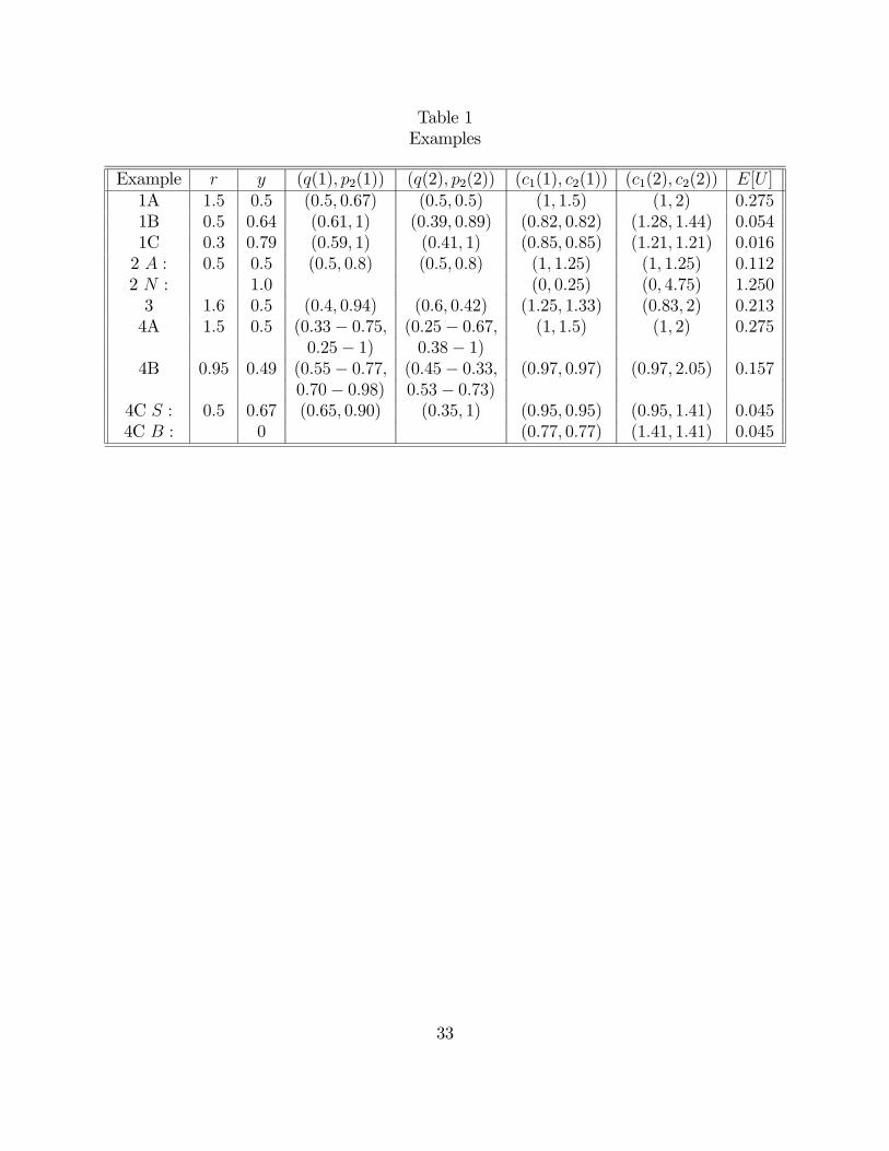
Table 1Examples

Example r y (q(1), p2(1)) (q(2), p2(2)) (c1(1), c2(1)) (c1(2), c2(2)) E[U ]1A 1.5 0.5 (0.5, 0.67) (0.5, 0.5) (1, 1.5) (1, 2) 0.2751B 0.5 0.64 (0.61, 1) (0.39, 0.89) (0.82, 0.82) (1.28, 1.44) 0.0541C 0.3 0.79 (0.59, 1) (0.41, 1) (0.85, 0.85) (1.21, 1.21) 0.0162 A : 0.5 0.5 (0.5, 0.8) (0.5, 0.8) (1, 1.25) (1, 1.25) 0.1122 N : 1.0 (0, 0.25) (0, 4.75) 1.2503 1.6 0.5 (0.4, 0.94) (0.6, 0.42) (1.25, 1.33) (0.83, 2) 0.2134A 1.5 0.5 (0.33− 0.75, (0.25− 0.67, (1, 1.5) (1, 2) 0.275

0.25− 1) 0.38− 1)4B 0.95 0.49 (0.55− 0.77, (0.45− 0.33, (0.97, 0.97) (0.97, 2.05) 0.157

0.70− 0.98) 0.53− 0.73)4C S : 0.5 0.67 (0.65, 0.90) (0.35, 1) (0.95, 0.95) (0.95, 1.41) 0.0454C B : 0 (0.77, 0.77) (1.41, 1.41) 0.045

33

References

Aghion, P., P. Bacchetta and A. Banerjee (2000). “Currency Crises and Monetary Policyin an Economy with Credit Constraints,” working paper, University College, London.

Allen, F. and D. Gale (1994). “Liquidity Preference, Market Participation and Asset PriceVolatility,” American Economic Review 84, 933-955.

– and – (1998). “Optimal Financial Crises,” Journal of Finance 53, 1245-1284.

– and – (1999). Comparing Financial Systems. Cambridge: MIT Press.

– and – (2000a). “Financial Contagion,” Journal of Political Economy 108, 1-33.

– and – (2000b). “Optimal Currency Crises” Carnegie-Rochester Conference Series onPublic Policy 53, 177-230.

– and – (2000c). “Banking and Markets Addendum: Prudential Regulation of Banks,”www.econ.nyu.edu/user/galed/papers.

Alonso, I. (1996). “On Avoiding Bank Runs,” Journal of Monetary Economics 37, 73-87.

Bernanke. B. and M. Gertler (1989). “Agency Costs, Net Worth, and Business Fluctua-tions,” American Economic Review 79, 14-31.

Bhattacharya, S. and D. Gale (1987). “Preference Shocks, Liquidity and Central BankPolicy,” inW. Barnett and K. Singleton, eds., New Approaches to Monetary Economics.New York: Cambridge University Press.

Bhattacharya, S. and A. Thakor (1993) “Contemporary Banking Theory,” Journal of Fi-nancial Intermediation 3, 2-50.

Bisin, A. and P. Gottardi (2000). “Decentralizing Incentive-Compatible Allocations inAdverse Selection Economies,” working paper, New York University.

Bryant, J. (1980). “A Model of Reserves, Bank Runs, and Deposit Insurance,” Journal ofBanking and Finance 4, 335-344.

Calvo, G. (1988). “Servicing the Public Debt: The Role of Expectations,” American Eco-nomic Review 78, 1411-1428.

Champ, B., B. Smith, and S. Williamson (1996). “Currency Elasticity and Banking Panics:Theory and Evidence,” Canadian Journal of Economics 29, 828-864.

Chang, R. and A. Velasco (2000). “Financial Fragility and the Exchange Rate Regime,”Journal of Economic Theory 92, 1-34.

34

– and – (2001). “A Model of Financial Crises in Emerging Markets,” Quarterly Journalof Economics 116, 489-517.

Chari, V. (1989). “Banking Without Deposit Insurance or Bank Panics: Lessons From aModel of the U.S. National Banking System,” Federal Reserve Bank of MinneapolisQuarterly Review 13 (Summer), 3-19.

– and R. Jagannathan (1988). “Banking Panics, Information, and Rational ExpectationsEquilibrium,” Journal of Finance 43, 749-60.

– and P. Kehoe (2000). “Financial Crises as Herds,” working paper, Federal Reserve Bankof Minneapolis.

Cole, H. and T. Kehoe (2000). “Self-Fulfilling Debt Crises,” Review of Economic Studies,67, 91-116.

Cone, K. (1983). Regulation of Depository Institutions. Stanford University Ph.D. disser-tation.

Corsetti, G., P. Pesenti and N. Roubini (1999). “Paper Tigers? A Model of the AsianCrisis,” European Economic Review 43, 1211-1236.

Diamond, D. (1997). “Liquidity, Banks and Markets,” Journal of Political Economy 105,928-956.

– and P. Dybvig (1983). “Bank Runs, Liquidity, and Deposit Insurance,” Journal ofPolitical Economy 91, 401-419.

– and R. Rajan (2001). “Liquidity Risk, Liquidity Creation and Financial Fragility: ATheory of Banking,” Journal of Political Economy 109, 287-327.

Flood, R. and N. Marion (1999). “Perspectives on Recent Currency Crises Literature,”International Journal of Finance and Economics 4, 1-26.

Geanakoplos, J. and H. Polemarchakis (1986). “Existence, Regularity, and ConstrainedSuboptimality of Competitive Allocations When the Asset Market Is Incomplete,” inWalter, Heller, Ross Starr, and David Starrett eds. Essays in honor of Kenneth J.Arrow: Volume 3, Uncertainty, information, and communication. Cambridge, NewYork and Sydney: Cambridge University Press, 65-95. Also reprinted in Debreu, Ger-ard, ed. (1996). General equilibrium theory. Volume 2. Elgar Reference Collection.International Library of Critical Writings in Economics, no. 67. Cheltenham, U.K.:Elgar; distributed by Ashgate, Brookfield, Vt. 67-97.

Gromb, D. and D. Vayanos (2001). “Equilibrium and Welfare in Markets with FinanciallyConstrained Abitrageurs,” working paper, MIT Sloan School of Management.

35

Grossman, S. and O. Hart (1983). “An Analysis of the Principal-Agent Problem,” Econo-metrica 51, 7-45.

Hellwig, M. (1994). “Liquidity Provision, Banking, and the Allocation of Interest RateRisk,” European Economic Review 38, 1363-1389.

– (1998). “Banks, Markets, and the Allocation of Risks in an Economy,” Journal ofInstitutional and Theoretical Economics 154, 328-345.

Jacklin, C. (1986). “Demand Deposits, Trading Restrictions, and Risk Sharing,” in E.Prescott and N.Wallace, eds., Contractual Arrangements for Intertemporal Trade (Uni-versity of Minnesota Press, Minneapolis, MN).

– and S. Bhattacharya (1988). “Distinguishing Panics and Information-Based Bank Runs:Welfare and Policy Implications,” Journal of Political Economy 96, 568-592.

Krugman, P. (1979). “A Model of Balance-of-Payments Crises,” Journal of Money Creditand Banking 11, 311-325.

Martin, A. (2000). “Liquidity Provision vs. Deposit Insurance: Preventing Bank Panicswithout Moral Hazard,” working paper, Federal Reserve Bank of Minneapolis.

Matutes, C. and X. Vives (1996). “Competition for Deposits, Fragility, and Insurance,”Journal of Financial Intermediation 5, 184-216.

– and – (2000). “Imperfect Competition, Risk Taking, and Regulation in Banking,”European Economic Review 44, 1-34.

Morris, S. (2000). “Contagion,” Review of Economic Studies 67, 57-78.

Morris, S. and H. S. Shin (1998). “Unique Equilibrium in a Model of Self-Fulfilling CurrencyAttacks,” American Economic Review 88, 587-597.

Morris, S. and H. S. Shin (2000). “Global Games: Theory and Applications,” workingpaper, Yale University.

Obstfeld, M. (1986). “Rational and Self-Fulfilling Balance of Payments Crises,” AmericanEconomic Review 76, 72-81.

Peck, J. and K. Shell (1999). “Bank Portfolio Restrictions and Equilibrium Bank Runs,”working paper, Cornell University.

Postlewaite, A. and X. Vives (1987). “Bank Runs as an Equilibrium Phenomenon,” Journalof Political Economy 95, 485-491.

Prescott, E. and R. Townsend (1984a). “Pareto Optima and Competitive Equilibria withAdverse Selection and Moral Hazard, Econometrica 52, 21-45.

36

Prescott, E. and R. Townsend (1984b). “General Competitive Analysis in an Economywith Private Information,” International Economic Review 25, 1-20.

von Thadden, E.-L. (1999). “Liquidity Creation through Banks and Markets: MultipleInsurance and Limited Market Access,” European Economic Review 43, 991-1006.

Wallace, N. (1988). “Another Attempt to Explain an Illiquid Banking System: The Di-amond and Dybvig Model with Sequential Service Taken Seriously,” Federal ReserveBank of Minneapolis Quarterly Review 12 (Fall), 3-16.

Wallace, N., (1990). “A Banking Model in which Partial Suspension is Best,” FederalReserve Bank of Minneapolis Quarterly Review 14 (Fall), 11-23.

Zame, W. (1993). “Efficiency and the Role of Default when Security Markets are Incom-plete,” American Economic Review 83, 1142-1164.

37