
Financial Regulation in a Quantitative Model of theModern Banking System∗
Juliane BegenauHarvard University
Tim LandvoigtUniversity of Texas at Austin
December 2015
Abstract
This paper builds a general equilibrium model with commercial banks and shadowbanks to study the unintended consequences of capital requirements. In particular,we investigate how the shadow banking system responds to commercial bank capitalregulation changes. A key feature of our model are defaultable bank liabilities thatprovide liquidity services to households. While the debt of commercial banks is insuredand therefore delivers the full value of liquidity services to households, shadow banks’debt is uninsured. Its value depends on the expected default rate of shadow banks.Commercial banks are subject to a capital requirement. Tightening the requirementfrom the status quo, leads households to substitute shadow bank liquidity for commer-cial bank liquidity and therefore to more shadow banking activity in the economy. Butthis relationship is non-monotonic due to an endogenous leverage constraint on shadowbanks that limits their ability to deliver liquidity services. The basic trade-off of ahigher requirement is between bank liquidity provision and stability. Calibrating themodel to data from the Financial Accounts of the U.S. and commercial banks’ regula-tory fillings, the optimal capital requirement is around 20%.
∗First draft: December 2015. Email addresses: [email protected], [email protected] would like to thank participants at the 2015 CITE conference on New Quantitative Models of FinancialMarkets, the Federal Reserve Bank of Boston, and the University of Texas at Austin.
1

1 Introduction
Unintended consequences are a challenging aspect of macroprudential financial regulation.
More stringent regulation of one sector can potentially strengthen its unregulated competi-
tors. For example, Regulation Q posed a cap on deposit rates. This made the creation
of institutions that provided alternatives to deposit accounts, such as money market mu-
tual funds, more attractive during periods of high interest rates (see Adrian and Ashcraft
(2012)). The construction of asset-backed commercial paper conduits represents an example
for regulatory capital arbitrage (see Acharya, Schnabl, and Suarez (2013)). Thus, banking
regulation has not only effects on targeted depository institutions but also on their compet-
itive environment, i.e. shadow banks. Shadow banks are financial institutions that share
features of depository institutions, e.g. in terms of their liability side such as money market
mutual funds or in terms of assets such as asset-backed security issuers and finance compa-
nies. At the same time, they are not subject to the same regulatory supervision as traditional
banks. A tightening of regulatory measures on traditional banks such as capital requirements
can shift activity to shadow banks, potentially increasing the fragility of the entire financial
system. In this paper, we study and quantify the effects of capital requirements in a general
equilibrium model with regulated (commercial) and unregulated (shadow) banks.
Our general equilibrium model features an endowment economy with households, regulated
(commercial) banks, unregulated (shadow) banks, and a regulator. The general equilibrium
environment is key to analyze the potential side effects of new policies. The main features
of our model are heterogeneous banks that make productive investments, can default on
their debt, and differ in their ability to guarantee the safety of their liabilities, as well as
household preferences for safe and liquid assets in the form of bank debt whose value to
households depends on their safety. While commercial bank debt is insured, shadow bank
2
debt is not. Two trees produce a stochastic endowment. Households have only access to one
tree. Shadow banks and commercial banks compete over shares and intermediate access to
the second tree. Matching the model to data from the Flow of Funds and the FDIC, we find
an optimal capital requirement that is substantially higher compared to current regulation.
The optimal level trades-off the reduction in liquidity provision, against an increase in the
safety of the financial system and consumption.
Key to this result is the model’s mechanism that pins down the relative size of the two
banking sectors. Shadow banks cannot guarantee the safety of their liabilities and therefore
face an endogenous leverage constraint. That is, the price at which they issue debt takes
into account the default probability implied by their leverage choice. The guarantee on their
debt gives commercial banks an advantage in producing liquidity services over shadow banks.
However, as long as commercial bank debt and shadow bank debt are imperfect substitutes,
shadow banks exists. The relative size is mainly determined by the value of their liquidity
services, which does not only depend on the total amount but also on the relative mix
between the two types of bank debt providing these services. With imperfect substitutable
bank liabilities, households like to consume some fraction of their liquidity services from
shadow bank debt as well.
We find that higher capital requirement on regulated banks shifts intermediation activity
from regulated to unregulated banks. When banks default, a fraction of the remaining bank
value is lost. A higher capital requirement forces commercial banks to lower their leverage,
effectively reducing their ability to produce liquidity services. At the same time, they become
safer, reducing expected deadweight losses associated with their failure. The reduction of liq-
uidity production by commercial banks increases the attractiveness of shadow bank liabilities.
Because shadow banks face an endogenous leverage constraint, they can only produce more
liquidity services by lowering their leverage and at the same time increasing their holdings of
3
the intermediated assets. In the process, shadow banks become also safer, reducing expected
deadweight losses to a minimum in the economy and thus increasing consumption. Liquidity
services are decreasing in the capital requirement because given a particular leverage ratio,
shadow banks can never produce the same amount of liquidity services compared to com-
mercial banks as the former always take into account their default probability. The optimal
requirement finds the welfare maximizing balance between a reduction in liquidity services
and the increase in the safety of the financial sector and consumption.
In addition, the simulated dynamic model shows that a greater capital requirement for
commercial banks reduces the volatility of asset prices, liquidity provision, and consumption.
The reduction in the volatility of consumption is another source of welfare gains to households
from increased capital requirements.
The equilibrium in this paper also features excessive liquidity creation by shadow banks
and procyclical shadow banking activity. The failure rate of shadow banks affects households’
valuation of shadow bank debt. In essence, the riskier shadow banks are, the lower the
liquidity services that households can derive from shadow bank debt. Shadow banks do not
internalize this effect on the liquidity value of their liabilities for households, which causes
them to issue too much debt. It further causes procyclical shadow banking activity: positive
aggregate shocks make shadow banks safer and therefore their debt more attractive. This
increases the share of shadow banking activity in good states of the world.
We match the model to aggregate data from the Flow of Funds on financial positions of
U.S. households and financial institutions, interest rates from FRED, as well as microdata
from U.S. depository institutions (FDIC bank call reports). We also use industry reports
to obtain estimates for the share of credit by each financial institution type as well as their
default and recovery rates on bonds. The key parameters are those that determine the
relative size of the two sectors and the spread between their debt securities: the elasticity
4

of substitution between the two types of banking sector debts as well as the parameter that
governs the sensitivity of liquidity services to the default rate of shadow banks. It’s intuitive
to think of commercial bank debt (mostly deposits, but also commercial paper, repo etc)
and shadow bank debt (mostly money market mutual fund shares, commercial paper, repo,
etc) as being slightly different securities. The elasticity of substitution parameter is pinned
down by the relative size of depository institution debt to shadow bank debt from the Flow
of Funds. The shadow bank liquidity value parameter in households’ utility function pins
down the 3-month spread between AA commercial paper for financial institutions and the
implied interest rate on depository institution debt from FDIC reports.
2 The main mechanism in a two period model
This section demonstrates the main mechanisms of our dynamic general equilibrium model
in a two-period model. We first describe the two-period model and the forces that determine
the optimal capital requirement. We discuss the key assumptions of the model in a separate
section.
Households maximize utility from consuming goods and liquidity services. The economy
receives two endowments of goods: one that households directly receive as income and one
that households can only access through financial intermediaries. Two types of intermedi-
aries, C-banks and S-banks, can perform the intermediation. They issue short-term debt to
households to fund the intermediated asset. The short term debt of both banks provides
households with liquidity services.
Both type of banks can declare bankruptcy and default on their debt. However, the debt
of C-banks is riskfree to households since the government provides deposit insurance for
these types of banks. In return, C-banks are subject to capital regulation. S-banks, on the
5
other hand, are not subject to regulation that limits their leverage. But their debt is risky
for households since debt of defaulting S-banks only pays off a fraction of the face value.
S-banks take into account the effect of their leverage choice on the expected payoff of their
debt, and hence endogenously choose to limit their leverage.
2.1 Description of the model
Endowments There are two periods. Households receive an income of Y0 at date 0 and
Y1 at date 1. Further, the intermediated asset is in unit supply and pays off Z at date 1. Y0
is known at date 0 whereas Y1 and Z are stochastic. In particular, trees Z and Y1 have two
realizations G = good and B = bad. Banks are exposed to idiosyncratic valuation shocks ρji
that are uniformly distributed on the interval [ρj, ρj] for bank types j = S,C, respectively.
The shocks ρji are independent of the endowment processes Y1 and Z.
Shadow banks There is a unit mass of S-banks. S-bank i chooses ASi shares of the Z-tree
at the beginning of period 0. The shares trade at a market price of p0. The tree has a
stochastic payoff of Z in period 1. To fund their investment, S-banks issue short term debt
BSi that trades at the price qSi . All trades occur in 0, so all prices must be 0 in t = 1. At the
beginning of period 1, S−banks face idiosyncratic valuation risks ρSi that are proportional to
their assets, with ρSi ∼ F Sρ , i.i.d. across banks. After a large realization of ρSi , S−bank i may
find it optimal to declare bankruptcy. In case of a bankruptcy, the bank’s equity is wiped
out, and its assets are seized by its creditors. In case the bank does not default, it returns
the debt it ows and pays out dividends to households.
The problem for shadow bank i is
V Si = max
ASi ,B
Si
q(ASi , B
Si )B
Si − p0A
Si
+E0
[M(max
{0, ZAS
i −BSi − ρSi A
Si
})].
6

Since ρSi is uniformly distributed, the probability that bank i with assets ASi and debt BS
i
stays in business is given by the probability that ρSi ≤ Z − BSi
ASi, i.e.
F Sρ
(Z − BS
i
ASi
)=Z − BS
i
ASi− ρS
ρS − ρS. (1)
The bank problem has constant returns to scale in AS, allowing for direct aggregation. Since
there is a unit mass of S− banks, we can directly interpret F S as the mass of banks that
do not fail. To further simplify the problem, we exploit the homogeneity in the scale of the
bank AS by defining leverage per asset bSi = BSi /A
Si .
Dropping the i−subscript, we can hence rewrite the problem as
V S = maxAS≥0,bS
ASvS(bS)
where1
vS(bS) = qS(bS)bS − p0 + E0
[M(F Sρ
(Z − bS − ρ−S
))]. (2)
In the above expression, ρ−S is the expected value of ρSi conditional on S− bank’s survival and
a realization of the random variable Z. We define ρ+S as the expected value of ρ conditional
on S−bank’s failure. Investors who hold debt issued by S-banks that go bankrupt recover a
fraction of each bond’s value
rS = (1− ξS)AS(Z − ρ+S
)BS
= (1− ξS)Z − ρ+SbS
. (3)
The date-0 dividend payments are equal to the initial equity required by the bank,
DS0 = AS(p0 − qSbS).
and the date-1 dividends are the payout amounts of the non-bankrupt banks:
DS1 = F SAS(Z − bS − ρ−S ).
1We describe the derivation in more detail in the appendix section A.1.
7

Commercial banks The problem of C-banks is similar to the S-bank problem, with the
important difference that C−banks are subject to a leverage constraint. Moreover, they have
to pay regulators the fee κ per unit of debt to fund the insurance. Defining bC = BC/AC , we
can write the problem for a C−bank as
V C = maxAC ,bC
ACvC(bC)
subject to
bC ≤ (1− θ)p0,
where
vC(bC) =(qC − κ
)bC − p0 + E0
[M(FCρ
(Z − bC − ρ−C
))]. (4)
The term ρ−C in the expression above is defined analogously to the S− banks.
Households who invest in C-bank debt always receive the full face value of the bonds. The
difference between the face value and the recovery value of the bonds for failing C-banks is
provided by the government (deposit insurance). The insurance fund recovers a fraction of
the value of the debt of bankrupt C-banks, per bond issued:
rC = (1− ξC)AC(Z − ρ+C)
BC= (1− ξC)
Z − ρ+CbC
.
As S−banks, C−banks payout DC0 and DC
1 in period 0 and 1, respectively.
Households In period 0, households have logarithmic utility over consumption C0. In
period 1, they have logarithmic utility over consumption C1 and power utility over liquidity
services H. The value function of households is
U(C0, C1, NS, NC) =
{log(C0) + β
(log(C1) + ψ (H/C1)
1−η
1−η
)for η ¿ 1
log(C0) + β (log(C1) + ψ log (H/C1)) for η=1,(5)
8
where η ≥ 1. Liquidity is a composite good (consisting of NS and NC) that is produced in
equilibrium by both types of intermediaries
H(NS, NC
)=
{[(1− ν)
(NS)α + ν
(NC)α]1/α
for α =1(NS)(1−ν)
(NC)ν
for α=1,
where α parameterizes the elasticity of substitution between liquidity services of both types of
banks. Weight ν determines the quality of liquidity services provided by C-banks relative to S-
banks. The weight ν depends on the fraction of defaulting S-banks F S, i.e. ν = 1/(1+(F S)ν),
and consequently
1− ν =(F S)ν
1 + (F S)ν.
Households maximize utility in equation (5) by choosing consumption C0, C1, and liquidity
services from each bank NS, NC , subject to the budget constraints
C0 = Y0 −∑j
Dj0 −
∑j
qjN j,
C1 = Y1 +∑j
Dj1 +NC +NS(F S + (1− F S)rs)− T.
In period 1, households have to pay a lump-sum tax of T that the government raises to
make whole the depositors of failed C-banks. Households are the sole owners of all banks
and therefore receive the dividend payments both at date 0 and date 1.
Government The government pays out on deposit insurance to reimburse depositors of
C-banks. The government covers the deficit by imposing a lump-sum tax on households in
period 1. Therefore the amount of tax funds the government raises is
T = BC [(1− FC)(1− rC)− κ].
9

Markets Asset market clearing in period zero requires
1 = AS + AC
NS = BS
NC = BC .
This implies for the goods market in period 1
C1 = Y1 + Z −∑j
Aj[Eρ(ρj) + ξj(1− F j)(Z − ρ+j )
]. (6)
2.2 Discussion of assumptions
The following paragraphs discuss key assumptions of the model.
Banks’ Role as Intermediaries In the model, banks are special because they provide
liquidity (discussed below) and intermediate assets. The role of banks as intermediaries
can be derived from first principles in numerous ways. For example, in models with asym-
metric information between borrowers and lenders, lenders with access to a cheaper screen-
ing or monitoring technology than other lenders (regular households) become banks (see
Freixas and Rochet (1998) for many other examples).
The Role of Banks as Liquidity Providers In this model, households value bank debt
because it is liquid2 and safe, an interpretation of bank debt in Gorton and Pennacchi (1990)
and in Gorton et al. (2012). The notion of safe and liquid assets includes bank deposits,
money market fund shares, commercial paper, repos, short-term interbank loans, Treasuries,
agency and municipal debt, securitized debt, and high-grade financial sector corporate debt.
2The idea to view banks as liquidity provider goes back to Diamond and Dybvig (1983). Other work hasbuilt upon this idea (e.g. Gorton and Pennacchi (1990))
10

Aside from the government, commercial banks and shadow banks are the most important
providers of these securities.3 The savings glut hypothesis articulated in Bernanke (2005) and
other recent work (e.g. Caballero and Krishnamurthy (2009), Gorton, Lewellen, and Metrick
(2012), Gourinchas and Jeanne (2012), and Krishnamurthy and Vissing-Jorgensen (2012))
rests on the notion that there exists a demand for safe and liquid securities. Economic
agents demanding these assets are for example households that hold deposits for transac-
tion or liquidity reasons as well as corporations, institutional investors, and high net worth
individuals that carry large cash-balances and seek safe and liquid investment vehicles with
higher yields than deposits, such as money market mutual funds. Commercial banks provide
mostly deposits, but also issue money market fund shares, repos, and commercial paper.
Some of these securities that commercial banks hold (most notably deposits) are explicitly
insured through deposit insurance. Others, such as money market fund shares and commer-
cial papers are indirectly insured due to government guarantees.4 Shadow banks generally
do not benefit from government guarantees, but nevertheless carry the characteristics of safe
and liquid assets during normal times.
In the model, liquidity servives are generated through debt issued by shadow banks and
commercial banks. Commercial bank debt represents all commercial bank liabilities precisely
because the demand for safe and liquid assets goes beyond merely deposits. We apply the
same idea to shadow bank debt with one notable difference: the value of shadow bank
liabilities depends on the likelihood at which shadow banks default.
3Historically, money market mutual funds (a type of shadow bank) emerged precisely to satisfy demandfor safe and liquid assets when Regulation Q imposed a ceiling on deposit rates.
4A number of empirical papers presents evidence for market expectations for government guarantees onU.S. banks (see for instance Flannery and Sorescu (1996), Kelly, Lustig, and Van Nieuwerburgh (2011), andGandhi and Lustig (2013)).
11
Liquidity services in households preference We capture the idea that bank liabilities
provide liquidity services with our utility specification. The households in our model represent
a blend of different agents with demands for different types of safe and liquid assets (deposits,
money market mutal fund shares, and so forth) provided by all financial institutions. This
is why our utility specification aggregates the liquidity services of both bank types.
Commercial bank debt always provides liquidity services no matter their default proba-
bility. This is different for shadow banks as the value from their liquidity service depends
on their probability of default. This captures the idea that shadow bank debt is only safe as
long as shadow banks are safe, that is, not too many of them go bankrupt.
The demand for liquidity services is captured with a money-in-the-utility function specifi-
cation. Since Sidrauski (1967) money-in-the-utility specifications have been used to capture
the benefits from money-like-securities for households in macroeconomic models. Feenstra
(1986) proved the functional equivalence of models with money-in-the-utility and models with
transaction or liquidity costs. The specific functional form is a version of Poterba and Rotemberg
(1986) and Christiano, Motto, and Rostagno (2010).5 We further assumed (η ≥ 1) comple-
mentarity between consumption and liquidity. This is intuitive as higher consumption levels
go along with higher transaction volumes and higher savings demand.
2.3 Equilibrium Characterization
Households The stochastic discount factor M1 equals
M = βE0
[C0
C1
(1− ψ
(H
C1
)1−η)]
.
Its first term is the standard discount factor implied by log utility, while the second term
reflects the adjustment to the discount factor resulting from the complementarity between
5In Christiano, Motto, and Rostagno (2010), the money and deposit utility parameter relates to the bankdebt-consumption elasticity η in the following way: σq = 2− η.
12
liquidity services and consumption.
MRSC = νU1
U2
(H
NC
)1−α
and MRSS = (1− ν)U1
U2
(H
NS
)1−α
denote the marginal rates of substitution between consumption and liquidity services by
C−banks and S−banks respectively.
The solution to the HH’s problem is characterized by the two FOCs for deposits, which
are also the HH’s intertemporal Euler equations. The FOC for C-bank deposits NC is
qC = E0
[M(1 +MRSC
)]. (7)
The first term on the RHS of equation (7) is the marginal utility from consuming the payoff of
1 per C-bank deposit bond purchased at time 0. MRSC is the marginal utility from liquidity
services.
The FOC for S-bank deposits NS is
qS = E0
[M[F Sρ +
(1− F S
ρ
)r +MRSS
]](8)
The payoff of one deposit bond issued by S-banks depends on the fraction of surviving banks
F S. For surviving banks, the payoff is simply 1 as for C-bank deposits. For failing banks,
it is given by the recovery value per bond rS. The second term, the marginal utility from
liquidity services, is analogous to C-banks.
Bank Portfolio Choices The optimal choice of asset purchases Aj for each bank type
j = C, S imply
vj(bj) = 0, (9)
13

for any Aj > 0. We can think of condition (9) as determining the relative size of the j-bank
sector. To see this, we show in appendix A that these conditions can be rewritten as
p0 − (qC − κ)bC =E0
(M
√12
2σC(FC)2
), (10)
p0 − qSbS =E0
(M
√12
2σS(F S)2
). (11)
where σj is the standard deviation of ρj.
The FOC for leverage per unit of assets bC is
(vC)′(bC) = 0.
In appendix A, we show that this condition can be expressed as
qC = λC + E0
(M FC
). (12)
This implies that the Lagrange multiplier on C-banks’ leverage constraint is always positive
as long as the marginal value of C-bank liquidity is positive.
The positive multiplier implies a binding constraint, i.e.
bC = (1− θ)p0.
As for C-banks, S-bank leverage per unit of assets is determined trough S-banks’ FOC for
bS
(vS)′(bS) = 0,
which can be written as
qS + bS∂qS(bS)
∂bS= E0
(M1F
S). (13)
Comparing the FOC for C-bank leverage in (12) to the S-bank FOC in (13) above reveals
the fundamental difference between the two types of banks. While C-banks are subject to a
14
constant leverage constraint that in equilibrium is always binding, S-banks choose to limit
their leverage because they internalize the effect of their leverage choice on the price of their
deposits, qS.
Increasing leverage bS will decrease the survival probability F S and hence lower the value
of S-bank deposits to HH, implying ∂qS(bS)∂bS
< 0, as can be seen in equation (8).
When choosing leverage, we assume that shadow banks take into account that their default
risk is priced. In this sense, each shadow bank acts as a monopolist for its own debt. But
it does not internalize how its leverage choice and default risk affects the value of liquidity
services for households. This is intuitive, as shadow bank bond prices are sensitive to the
specific default risk of the issuer. But they also move with changes in aggregate liquidity
conditions, which are caused by actions of all shadow banks, but not by any individual bank.
Thus, it is best to think of the changes in the value of aggregate liquidity services as an
externality arising in general equilibrium.
The following proposition that we prove in the appendix states the resulting endogenous
leverage choice of S-banks:
Proposition. Leverage per units of assets bS of S-banks is
bS = E0
(M
√12σSξS
(1− ν)
(1− ψ (H/C1)
1−η
ψ (H/C1) −η
)(H
NS
)1−α). (14)
For any reasonable parameter combinations, the above equilibrium choices of asset pur-
chases and leverage for both types of banks imply that C−banks have a dominant position
in the intermediated asset (AC > AS). The intuitive reason for this equilibrium outcome is
as follows.
First, C-banks’ debt is insured and therefore C-vanks do not internalize the effect of their
leverage choice on the price of their debt. Since the marginal liquidity benefit is always
15
positive, C-banks always exhaust their leverage constraint. S-banks, however, do internalize
the increase in their default risk. Hence, if C-banks and S-banks are fundamentally equally
risky, S-banks choose lower leverage6. Required initial equity for C-banks is p0 − qCbC .
Leverage bC is a constant fraction the asset price by the collateral constraint and higher than
that of S-banks if θ is sufficiently small. Then the bond price qC must adjust in equilibrium in
order for required initial equity to be equal the expected dividend. For reasonable parameter
combinations, this in turn means that the marginal benefit of C-bank debt to households
must be lower than that of S-bank debt. If debt is further sufficiently substitutable, this
means that C-banks must hold a greater share of the intermediated asset in equilibrium7.
Size of the Banking Sectors & Procyclical Shadow Banking Activity The exact
split between both types of banks depends on several parameters, particularly the elasticity
of substitution between both kinds of liquidity α.
The relative size of both banking sectors is determined in equilibrium by the marginal
benefit of opening each bank in this period and receiving dividends next period. Mathemat-
ically, this means that the holdings of the intermediated asset by both types of banks, AC
and AS, and thus the relative size of both banking sectors, are jointly determined by the
FOCs (10) and (11).
6This statement of course depends on the parameters of the model, in particular the value of θ, i.e. thetightness of C-banks’ leverage constraint. For any values close to the capital requirements of commercialbanks, we found this statement to be true.
7Even for equal shares of asset holdings (AS = AC), C-banks will produce NC > NS due to their higherleverage. If both types of debt are close to being complements, the higher leverage of C-banks by itself issufficient to create the lower marginal benefit. Thus the C-bank share is increasing in the elasticity parameterα.
16

0 0.05 0.1 0.15
C-bank
0.1
0.2
0.3
0.4
0.5
0.6A
S
Cost - good stateBenefit - good stateCost - bad stateBenefit - bad state
-0.6 -0.4 -0.2 0 0.2
S-bank
0.1
0.2
0.3
0.4
0.5
0.6
AS
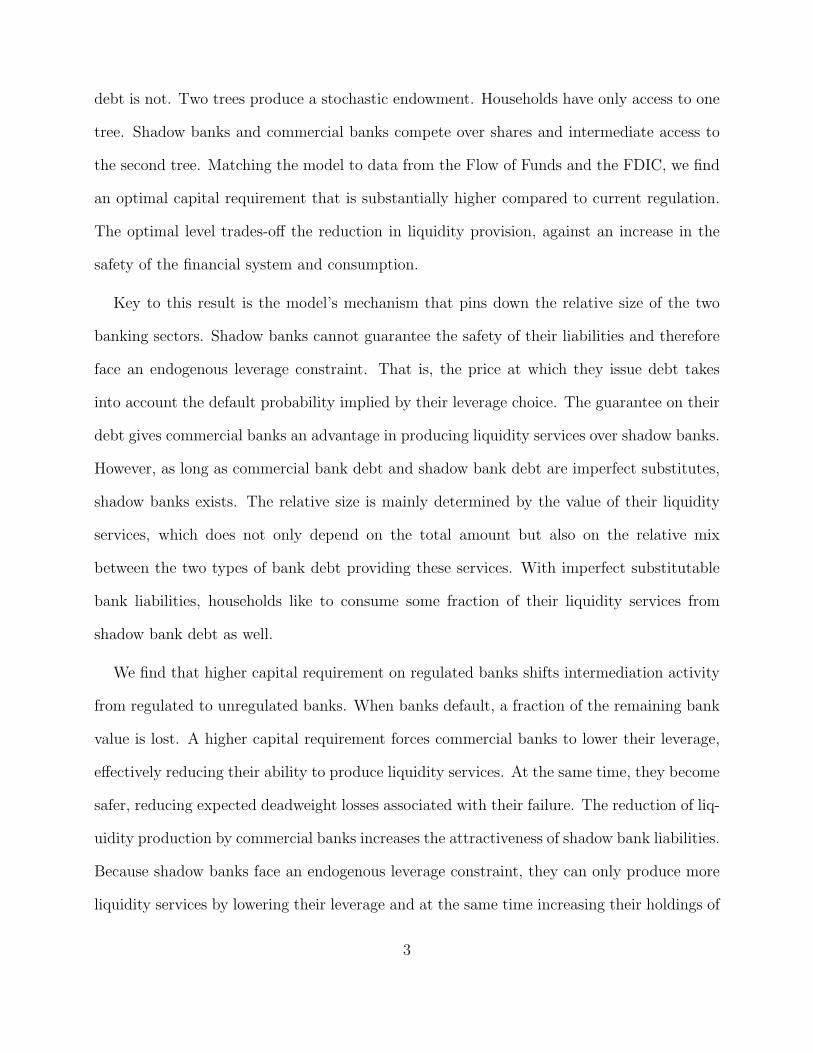
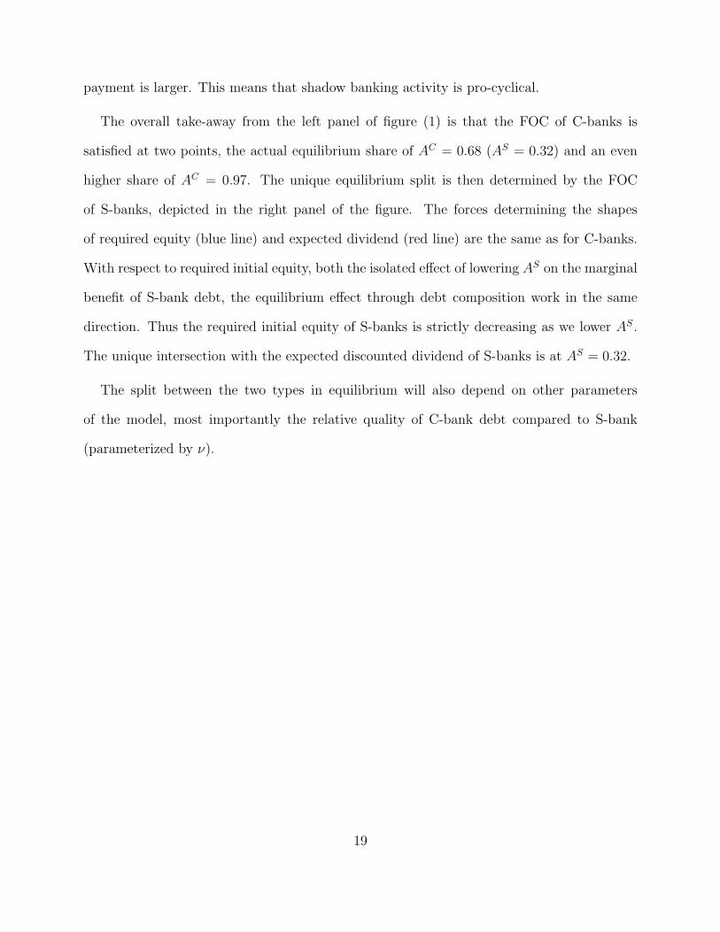
Figure 1: Equilibrium Determination of AC and AS for α = 1/3
Left-hand side (required equity at time 0, blue line) and right-hand side (expected dividendat time 1, red line) of banks’ first-order condition for asset holdings (Aj), while imposingmarket clearing 1 = AC + AS and holding fixed all other variables.
Figure (1) shows the LHS and RHS of both equations graphically for the calibrated model,
depending on the current state of the economy. We first numerically compute the equilibrium
values of all variables. Then we vary the share of S-banks and C-banks, AS and AC , while
holding all other variables fixed (and imposing market clearing AS +AC = 1). The blue lines
trace the value of the LHS of the first-order conditions (10) and (11) as we vary the shares,
p0−qjbj, for j = C, S, respectively. Holding constant p0 and bj, the only source of variation is
through the bond price qj. Since total debt issued by each type is given by asset share times
leverage per unit of assets, N j = bjAj, the marginal benefit of deposits of each type changes
as we vary the asset shares, as can be seen from the pricing equations for the qj, (7) and (8).
In particular, as we increase the share of type j holding total provided liquidity constant,
the marginal liquidity benefit of type j’s deposits will decline (for any α < 1), and therefore
type j’s bond price will also decline. This means that the equity required to purchase the
17

bank’s initial asset position becomes larger for the same face amount of debt issued.
An opposing effect is that, as long as liquidity services provided by both types of debt are
imperfect substitutes, the marginal benefit derived from each type’s debt is also affected by
the composition of the total debt. When we increase the share of C-banks, we decrease the
share of S-banks due to market clearing. Consequently the composition of liquidity services
becomes more unequal and the amount of services derived from total debt issued by both
banks declines, which leads to a general increase in the marginal benefit of both kinds of
liquidity. Both effects, the pure effect of an increase in AC and the equilibrium effect through
the implied decrease in AS can be seen in left panel of (1). Lowering AS from 0.5 to about
0.15 (= raising AC from 0.5 to 0.85) causes a decrease in the marginal benefit of C-bank
debt, which in turn lowers the bond price qC and therefore raises the required initial equity
of C-banks (the blue line in the graph). By lowering AS any further, the composition of debt
becomes so unequal that the marginal benefit of any liquidity rises again, causing both bond
prices (also qC) to increase again. Hence the required equity of C-banks bends backwards,
yielding the overall non-monotonic shape.
The effect on the RHS of equation (11) is depicted by the red lines and quantitatively
smaller. The discounted expected dividend at time 1 (per unit of assets) is only indirectly
affected by a variation in asset shares through the households’ discount factor which depends
on consumption C1. As the share is shifted towards C-banks, consumption C1 decreases
since S-banks have lower leverage and cause lower bankruptcy-induced consumption losses to
households. This decrease in C1 raises the discount factor, leading to a higher present value
of the expected dividend.
The share of shadow banking activity also depends on the economic state. In a boom
(solid line), shadow banks can issue debt at a higher price because they are less likely to
fail next period. Moreover, because the default probability is lower, the expected dividend
18
payment is larger. This means that shadow banking activity is pro-cyclical.
The overall take-away from the left panel of figure (1) is that the FOC of C-banks is
satisfied at two points, the actual equilibrium share of AC = 0.68 (AS = 0.32) and an even
higher share of AC = 0.97. The unique equilibrium split is then determined by the FOC
of S-banks, depicted in the right panel of the figure. The forces determining the shapes
of required equity (blue line) and expected dividend (red line) are the same as for C-banks.
With respect to required initial equity, both the isolated effect of lowering AS on the marginal
benefit of S-bank debt, the equilibrium effect through debt composition work in the same
direction. Thus the required initial equity of S-banks is strictly decreasing as we lower AS.
The unique intersection with the expected discounted dividend of S-banks is at AS = 0.32.
The split between the two types in equilibrium will also depend on other parameters
of the model, most importantly the relative quality of C-bank debt compared to S-bank
(parameterized by ν).
19
0 0.05 0.1 0.15
C-bank
0.1
0.2
0.3
0.4
0.5
0.6A
S
Cost - good stateBenefit - good stateCost - bad stateBenefit - bad state
0.06 0.08 0.1 0.12 0.14
S-bank
0.1
0.2
0.3
0.4
0.5
0.6
AS
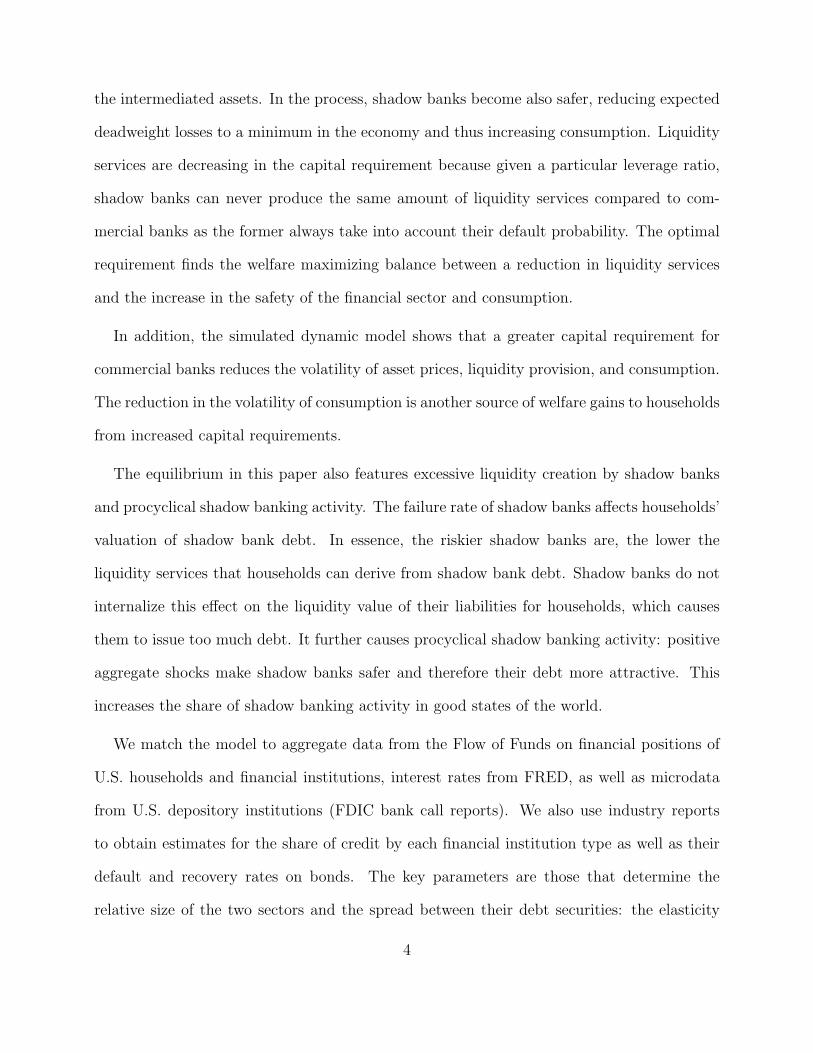
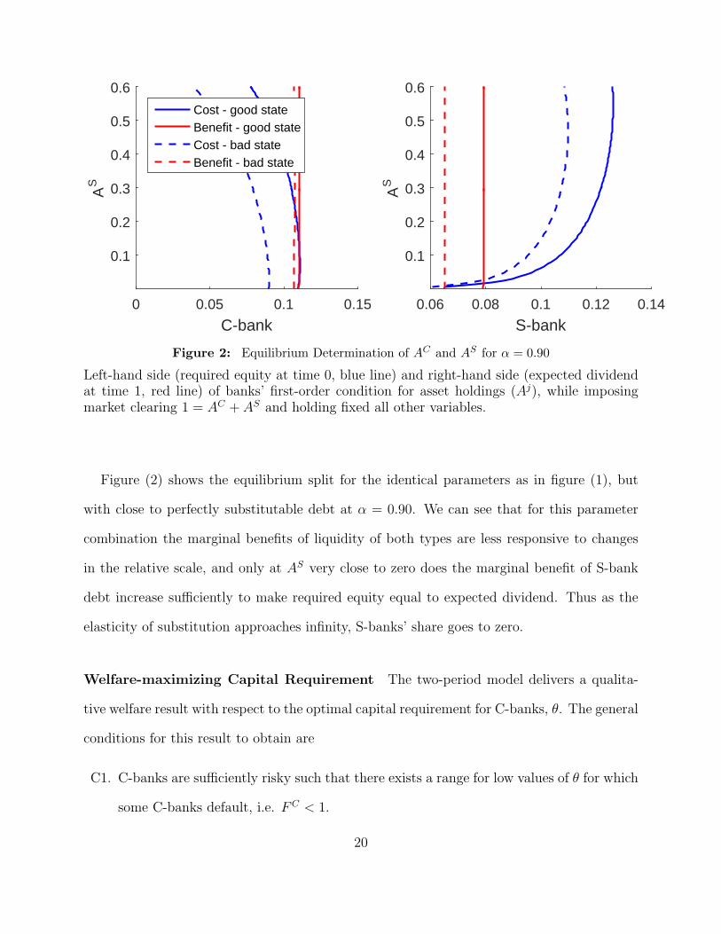
Figure 2: Equilibrium Determination of AC and AS for α = 0.90
Left-hand side (required equity at time 0, blue line) and right-hand side (expected dividendat time 1, red line) of banks’ first-order condition for asset holdings (Aj), while imposingmarket clearing 1 = AC + AS and holding fixed all other variables.
Figure (2) shows the equilibrium split for the identical parameters as in figure (1), but
with close to perfectly substitutable debt at α = 0.90. We can see that for this parameter
combination the marginal benefits of liquidity of both types are less responsive to changes
in the relative scale, and only at AS very close to zero does the marginal benefit of S-bank
debt increase sufficiently to make required equity equal to expected dividend. Thus as the
elasticity of substitution approaches infinity, S-banks’ share goes to zero.
Welfare-maximizing Capital Requirement The two-period model delivers a qualita-
tive welfare result with respect to the optimal capital requirement for C-banks, θ. The general
conditions for this result to obtain are
C1. C-banks are sufficiently risky such that there exists a range for low values of θ for which
some C-banks default, i.e. FC < 1.
20

C2. S-banks are at least as risky as C-banks; in other words, the standard deviation of their
idiosyncratic shocks σS is at least as large as that of C-banks.
C3. Households derive a strictly positive utility benefit from liquidity services (ψ > 0), and
the liquidity services provided by C-banks are at least as good as those of S-banks.
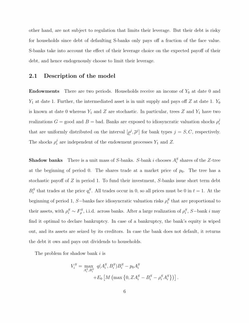
Under these fairly general conditions there exists a trade-off in the model that leads to a
unique utility maximum in θ. Figure (3) illustrates the trade-off: increasing the capital re-
quirement leads to an increase in numeraire consumption (top right graph), as fewer C-banks
default due to lower leverage and hence bankruptcy losses become smaller. At the same time,
decreasing C-bank leverage through tighter capital requirements lowers the amount of liquid-
ity services provided to households (bottom left), as a greater share of the intermediated asset
is shifted to S-banks. Since total utility is a weighted sum of both components, household
utility is maximized when C-banks have become completely safe (FC = 1) and no further
increase in consumption is possible (but liquidity decreases further with higher θ).
21

0.2 0.4 0.6
AC
0.55
0.6
0.65
0.7
0.75
0.8α = 0α = 0.25α = 0.5
0.2 0.4 0.6
C
1.575
1.58
1.585
1.59
1.595
1.6
θ
0.2 0.4 0.6
H
0.05
0.1
0.15
0.2
θ
0.2 0.4 0.6
U
-0.04
-0.02
0
0.02
0.04
0.06
Figure 3: Comparative Statics in Capital Requirement θ
Top left: share of C-banks, top right: consumption at time 1, bottom left: utility fromliquidity services, bottom right: total household utility.
3 Dynamic Model
This section presents the quantitative general equilibrium model.
22

3.1 Model Description
Agents and Environment Time is discrete and infinite. The agent, intermediary, and
endowment ownership structure is identical to the two-period model. The two types of
intermediaries finance Z−tree investments by issuing equity and debt to households. They
have limited liability, i.e., they can choose to declare bankruptcy.
S-Banks There is a unit mass of S-banks, indexed by i. S-bank i holds ASt,i shares of the
Z-tree at the beginning of period t. The shares trade at a market price of pt. To fund their
investment, S-banks can issue short term debt. The debt of S-bank i trades at the price qSt,i.
At the beginning of the period, S-bank i has BSt,i bonds outstanding.
There is an idiosyncratic component to the payoff of Z-shares when held by bank i.
Specifically, the payoff per share held by bank i is Zt. At the beginning of each period,
S-banks can decide to declare bankruptcy. Each period, they face idiosyncratic valuation
risks ρSt,i that are proportional to its assets. ρSt,i is an idiosyncratic loss with ρSt,i ∼ F Sρ , i.i.d.
across banks and time. In case of a bankruptcy, banks’ equity is wiped out, and their assets
are seized by their creditors.
Since the idiosyncratic valuation shocks are uncorrelated over time, it is convenient to
write bank i’s optimization problem after the bankruptcy decision, net of the idiosyncratic
payoff. Conditional on asset holdings ASt,i and debt BS
t,i, all banks have the same value and
face identical problems:
V S(BSt , A
St , Zt) = max
ASt+1,i,B
St+1,i
(Zt + pt − ρSt,i)−BSt,i + qSt B
St+1,i − ptA
St+1,i
+Et
[Mt,t+1V
S(ASt+1,i, B
St+1,i, Zt+1, ρ
St+1,i)
].
As in the two period model, the problem is again homogenous of degree one and identical for
each firm. We can omit subscripts i and define leverage bSt =BS
t
AStand asset growth aSt+1 =
ASt+1
ASt
23
and
vS(bSt , Zt) =V S(AS
t,i, BSt,i, Zt)
ASt,i
= maxaSt+1,b
St+1
Zt + pt − bSt + aSt+1
(qSt b
St+1 − pt + Et
[Mt,t+1v
S(bSt+1, Zt+1)]).
Using ρSt,i ’s independence of Zt the continuation value vS(bSt+1, Zt+1) is derived from
V S(ASt,i, B
St,i, Zt, ρ
St,i) = max{0, V (AS
t,i, BSt,i, Zt)− ρSt,iA
St,i}
= 1{ρSt,i≤
V S(ASt,i
,BSt,,Zt)
ASt,i
}
(V S(AS
t,i, BSt,i, Zt)− ρSt,iA
St,i
).
Taking the expectation with respect to ρ of the last line gives
V (ASt , B
St , Zt) = F S
ρ
(V S(AS
t , BSt , Zt)
ASt
)V (AS
t , BSt , Zt)− AS
t
ˆ V (ASt ,BS
t ,Zt)
ASt
ρ
ρ dFρ(ρ).
Since we take expectations over the idiosyncratic valuation shock, the problem is identical
for each bank and so
vS(bSt , Zt) =V S(AS
t,i, BSt,i, Zt)
ASt,i
.
C-Banks There is a unit mass of C-banks. C-banks are different from S-banks in two
ways: (i) they issue short-term debt that is insured and risk free from the perspective of
creditors, and (ii) they are subject to regulatory capital requirements. The pay an insurance
fee of κ for each bond they issue. The problem of all C banks is identical, thus we can drop
the subscript.
We can write the problem of C-bank i as
vC(bCt , Zt) =V C(AC
t , BCt , Zt)
ACt
= maxaCt+1,b
Ct+1
Zt + pt − bCt + aCt+1
(qCt b
Ct+1 − pt + Et
[Mt,t+1v
C(bCt+1, Zt+1)]).
subject to
(1− θ)Et[pt+1] ≥ bCt .
24

The continuation value Et
[Mt,t+1v
C(bCt , Zt+1)]is analogous to the continuation value of
shadow banks.
Bankruptcy The idiosyncratic asset valuation shock is realized just before the period
starts.
If a S-bank declares bankruptcy, its equity becomes worthless, and creditors seize all of
the banks assets. Before defining the recovery value, it is useful to define the expectations of
idiosyncratic bank losses conditional on survival or bankruptcy as
ρ−(vj(bjt)) = Eρ
[ρjt,i | ρ
jt,i < vj(bjt)
]for surviving banks, and
ρ+(vj(bjt)) = Eρ
[ρjt,i | ρ
jt,i > vj(bjt)
]for failing banks, for j = S,C respectively.
Banks that go bankrupt do no pay a dividend and their equity becomes worthless upon
bankruptcy. After their restructuring has completed, the bankrupt banks are replaced by new
banks who face the same forward-looking portfolio problem as existing banks. The recovery
amount per bond issued is hence
rj(bjt) = (1− ξj)Zt + pt − ρ+j(vj(bjt))
bjt,
with a fraction ξj lost in the bankruptcy proceedings. After the bankruptcy proceedings are
completed, and new shadow bank is set up to replace the bankrupt one. This bank sells its
equity to new owners, and is otherwise identical to an existing shadow bank with zero assets
and liabilities.
If a C-bank declares bankruptcy, its equity becomes worthless as well. The bank is then
taken over by the government that uses lump sum taxes and revenues from deposit insurance,
25

κBCt+1, to pay out the bank’s creditors in full. That is, lump sum taxes are defined
Tt = (1− FC(bCt ))(1− rC(bCt ))BCt − κBC
t+1.
The average dividend conditional on survival for S-banks
dSt =(Zt + pt − ρ−(vS(bSt+1))
)− bSt + aSt+1
(qSt b
St+1 − pt
),
and for C-banks
dCt =(Zt + pt − ρ−(vC(bCt+1))
)− bCt + aCt+1
(qCt b
Ct+1 − pt
).
Households Households derive utility from the consumption Ct of the fruit of both trees.
Households hold a portfolio of all securities that both types of intermediaries issue. In
particular, they buy equity shares of both types of intermediaries, Sjt , that trade at price of
pjt , for j = S,C respectively. They further buy the short terms bonds both types issue, N jt ,
trading at prices qjt , for j = S,C.
Households consume the liquidity services provided by the short term debt they hold at
the beginning of the period. This reflects that the liquidity services accrue at the time when
the deposits from last period are redeemed. Let N jt =´ 1
0N j
t,i di, for j = S,C. Then the total
liquidity services produced are
H(NSt−1, N
Ct−1),
and household utility in period t is
U(Ct, H(NSt−1, N
Ct−1)).
We specify utility as
U(Ct, H(NSt−1, N
Ct−1)) =
C1−γt − 1
1− γ+ ψ
(H(NS
t−1, NCt−1)/Ct
)1−η
1− η,
26

with
H(NSt−1, N
Ct−1) =
[ΛS,t(N
St−1)
α + ΛC,t(NCt−1)
α]1/α
.
The elasticity of substitution between the two types of bank liabilities is 1/(1− α).
We define the weights on the liquidity services of deposits of commercial banks ΛC,t and
shadow banks ΛS,t as follows:
ΛC,t =1
1 + F Sρ (vS (bSt ))
ν
ΛS,t =F Sρ
(vS(bSt))
ν
1 + F Sρ (vS (bSt ))
ν,
with ν > 0. The liquidity productivity of shadow banks is lower than that of commercial
banks. The discount depends on the fraction of surviving shadow banks. If both bank types
are equally safe, that is F Sρ
(vS(bSt))
= 1, the weights amount each to 1/2.
Denoting household wealth at the beginning of the period by Wt, the complete intertem-
poral problem of households is
V H(Wt, NSt−1, N
Ct−1, Yt) = max
Ct,NSt ,NC
t ,SSt ,SC
t
U(Ct, H(NSt−1, N
Ct−1)) + β Et
[V (Wt+1, N
St , N
Ct , Yt+1)
]subject to
Wt + Yt − Tt = Ct +∑j=S,C
pjtSjt +
∑j=S,C
qjtNjt (15)
Wt+1 =∑j=S,C
F jρ
(vj(bjt+1)
)(Dj
t+1 + pjt+1)Sjt
+NSt
[F Sρ
(vS(bSt+1)
)+(1− F S
ρ
(vS(bSt+1)
))rS(bSt+1)
]+NC
t . (16)
The budget constraint in equation (15) shows that households spend their wealth and income
on consumption and purchases of equity and debt of both types of intermediaries. The
securities issued are the same for all banks, independent of the previous bankruptcy status.
27
The equity purchases for banks that have gone through bankruptcy at the beginning of
period t can be understood as initial equity offerings for these banks, while the purchases of
equity of surviving banks are in a secondary market. However, since both new and surviving
banks hold identical portfolios, their securities have the same price and there is no need to
distinguish primary and secondary markets.8
Market Clearing Asset markets
ASt+1 + AC
t+1 = 1
BSt = NS
t−1
BCt = NC
t−1
SSt = 1
SCt = 1.
Resource constraint
Ct = Yt + Zt − µρ −∑j=S,C
ξj(Zt + pt − ρ+,jt )Aj
t
(1− F j
ρ
(vj(bjt)
)).
3.2 Equilibrium Conditions
Household The household’s first-order conditions for purchases of bank equity are, for
j = S,C,
pjt = Et
[Mt,t+1F
jρ
(vj(bjt+1)
)(Dj
t+1 + pjt+1)],
where we have defined the stochastic discount factor
Mt,t+1 = βU1(Ct+1, Ht+1)
U1(Ct, Ht).
8It is possible to show that the price to an equity claim of bank types j, pjt , is equal to the value of thatbank’s security portfolio, Aj
t+1pt − qjtBjt+1.
28
We further define the intratemporal marginal rate of substitution between consumption
and liquidity services
Qt =U2(Ct, Ht)
U1(Ct, Ht).
Then the first-order conditions for purchases of bonds of either type of bank are
qCt = Et
[Mt,t+1
(1 +Qt+1ΛC,t+1
(Ht+1
NCt
)1−α)]
, (17)
qSt = Et
{Mt,t+1
[F Sρ
(v(bSt+1)
)+(1− F S
ρ
(v(bSt+1)
))rS(bSt+1) +Qt+1ΛS,t+1
(Ht+1
NSt
)1−α]}
.
(18)
The payoff of commercial bank bonds is 1, whereas the payoff of shadow bank bonds
depends on their default probability and recovery value. The last terms in each expression
represent the marginal benefit of liquidity services to households.
Banks S-banks are subject to an endogenous borrowing constraint. Each S-banks is a
monopolist for its own debt, and hence internalizes the effect of supplying additional bonds
on the bond price.
Specifically, each S-bank views the price of its debt as a function of its supply of bonds
qSt = q(bSt+1) that is determined by households’ first order condition in equation 18.
It follows that the FOC of S-banks for leverage is
q(bSt+1) + bSt+1 q′(bSt+1) = Et
[Mt,t+1F
Sρ
(vS(bSt+1, Zt+1
))]. (19)
The partial derivative q′(bSt+1) can be obtained directly from households’ FOC for purchases
of shadow bank debt. In the appendix we show that differentiating equation (18) yields
q′(bSt+1) = −Et
{Mt,t+1
[fρ(v(bSt+1
)) (1− r
(bSt+1
))(20)
+(1− F S
ρ
(v(bSt+1
))) r(bSt+1)
bSt+1
+1− ξSbSt+1
fρ(v(bSt+1
)) (v(bSt+1
)− ρ+,S
t
)]}.
29

The RHS is strictly negative, implying that the price of shadow bank debt is decreasing in
shadow bank leverage bSt+1. The first term on the RHS is the loss for lenders from a marginal
increase in the probability of default. The second term reflects that the recovery value per
bond in case of bankruptcy is marginally decreased if the shadow bank issues more debt.
The third term is positive and captures that the conditional expectation of the idiosyncratic
losses of bankrupt firms decreases as leverage increases.
The debt price of commercial banks is independent of their leverage choice. Therefore the
FOC of C-banks for leverage is
qCt − κ =λCtaCt+1
+ Et
[Mt,t+1Fρ
(vC(bCt+1, Zt+1)
)].
with λCt being the Lagrange multiplier on the leverage constraint. This FOC and the house-
hold FOC for purchases of commercial bank debt (17) jointly imply that the Lagrange mul-
tiplier is positive and hence the C−bank leverage constraint is binding9, i.e.
(1− θ)Et[pt+1] = bCt .
3.3 Calibration
The stochastic process for the Y-tree is a AR(1) in logs
log(Yt+1) = (1− ρY )log(µY ) + ρY log(Yt) + ϵYt+1,
where ϵYt is i.i.d. with mean zero and volatility σY . To capture the correlation of asset payoffs
with fundamental income shocks, we model the payoff of the intermediated asset as
Zt = ϕY Yt exp(ϵZt ),
where ϵZt is i.i.d. with mean zero and volatility σZ , independent of ϵYt . This structure of the
shocks implies that Zt inherits all stochastic properties of aggregate income Yt, and is subject
9The constraint is binding if the marginal liquidity benefit from commercial bank debt is positive and thedeposit insurance fee is not too large. This is the case for all relevant parameter combinations.
30
to an additional temporary shock that reflects risks specific to intermediated assets, such as
credit risk.
We quantify the model with data from the Flow of Funds10, Compustat, and NIPA. We
use quarterly data from 1999 (after the passage of the Gramm-Leach-Bliley Act that revoked
parts of the Glass-Steagall Act) until the second quarter of 2015. We choose depository insti-
tutions as data counterparts for C−banks and shadow bank institutions as data counterparts
for S−banks. Shadow banks are defined on their asset side as security broker and dealer,
finance companies, insurance companies, asset-backed security issuers and so on and on their
liability side as money market mutual funds.
We normalize each bank’s balance sheet position, as well as consumption and safe asset
by total financial assets of each intermediary type. For C-Banks this amounts to dividing
by total depository institution financial assets. For S-Banks this means that we need to
aggregate total financial assets of all shadow-banking institutions from the Flow of Funds
tables.
10The Flow of Funds tables are organized according to institutions and instruments. We focus on thebalance sheet information on institutions. This is important, as we want to take into account all bank andshadow-bank positions when we quantify the model.
31

Table 1: Parametrization
Parameters Function Value Target
β discount rate 0.985 Literatureα maps into CES par. 1− 1/σelast = 0.1056 S−bank share GS report, 41%ψ utility weight on safe assets 0.016 S−bank book leverage 30ν liquidity factor 0.67 spread on C−& S−bank debt
CP AA fin.- FDIC r exp, 2.17%η compl. bw cons & safe assets 2 vol(consumption/safe assets)
κ deposit insurance fee 0.0006168 deposit ins. rates(25 bp p.a)θ C− bank capital req. 0.10 Effective Tier 1 cap ratioξCρ bankruptcy loss 0.72 recovery rate (37.1%)
ξSρ bankruptcy loss 0.48 recovery rate (37.1%)
µCρ mean of ρ shock 0 assumption
σCρ vol of ρ shock 0.1 FDIC default rate 0.42 %
µSρ mean of ρ shock 0 assumption
σSρ vol of ρ shock 0.2 qS : FRED CP ON AA fin. sector
σZ vol of Z shock 0.005µY mean of Y 0.1 normalizationρY persistence of Y 0.85 normalizationσY vol of Y shock 0.0025 agg. TFP vol
The key parameters are those that determine the relative size of the two sectors. These are
the elasticity of substitution of HH (α =1 − 1/elasticity) between the two liquidity services
provided by the two types of banking sector liabilities, and the sensitivity of liquidity services
provided by shadow banks to their default rate (ν).
It’s intuitive to think of commercial bank debt (mostly deposits, but also commercial pa-
per, repo etc) and shadow bank debt (mostly money market mutual fund shares, commercial
paper, repo, etc) as being slightly different securities. The elasticity of substitution param-
eter is pinned down by the relative size of depository institution debt to shadow bank debt
from the Flow of Funds. The shadow bank liquidity value parameter in households’ utility
function is determined by the 3-month spread between AA commercial paper for financial
32
institutions and the implied interest rate on depository institution debt from FDIC reports.
We set κ, the deposit insurance fee to 0.0006168. This is in the range of quarterly FDIC
assessment rates. The parameters ξS and ξC (loss in bankruptcy) are set to match the
average recovery value of 30.5 percent from Moody’s report.11 We set σCρ such that the
default probability of bank C equals that of the data. The FDIC publishes12 estimates for
average default probabilities of bank holding companies ( 0.4175 percent) for the 2006−2008
period13. We set σCρ such that the probability of default equals 4.2%. We set σS
ρ of shadow
banks idiosyncratic risk such that the price of shadow banking debt in the model, matches
the 3 month AA-rated financial sector commercial paper rate from FRED.
3.4 Results
We solve the dynamic model using second-order approximation around the model’s deter-
ministic steady state. We then simulate the model for many periods and compute moments
of the simulated series, for different values of the capital requirement θ. Table (2) reports
first and second moments for capital requirements ranging from 10% to 25%.
As for the two-period model, there is a unique maximum in aggregate welfare. The welfare
maximum for the quantitative model occurs in the interval between 22 and 23 percent. The
main forces leading to this result are the same as in the simple model. Increasing θ makes the
debt of both types of banks safer, thus reducing bankruptcy losses and increasing aggregate
consumption. At the same time, a higher level of θ restricts the amount of liabilities and
thus liquidity commercial banks can produce for each unit of assets.
11We use Moody’s 1984-2004 report. Exhibit 9 in the report presents the recovery rates of defaulted bondfor financial institutions. We use the mean for financial institutions over all bonds and preferred stocks.
12We take the average default probability from table 1 on the FDIC website.13 That is 0.13+3.21
8 = 0.4175
33
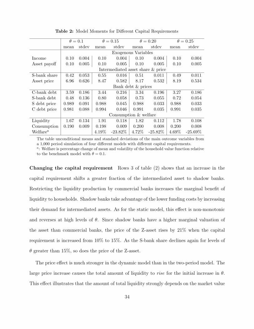
Table 2: Model Moments for Different Capital Requirements
θ = 0.1 θ = 0.15 θ = 0.20 θ = 0.25mean stdev mean stdev mean stdev mean stdev
Exogenous VariablesIncome 0.10 0.004 0.10 0.004 0.10 0.004 0.10 0.004Asset payoff 0.10 0.005 0.10 0.005 0.10 0.005 0.10 0.005
Intermediated asset share & price
S-bank share 0.42 0.053 0.55 0.016 0.51 0.011 0.49 0.011Asset price 6.96 0.626 8.47 0.582 8.17 0.532 8.19 0.534
Bank debt & prices
C-bank debt 3.59 0.186 3.44 0.216 3.34 0.196 3.27 0.186S-bank debt 0.48 0.136 0.80 0.058 0.73 0.055 0.72 0.054S debt price 0.989 0.091 0.988 0.045 0.988 0.033 0.988 0.033C debt price 0.981 0.088 0.994 0.046 0.991 0.035 0.991 0.035
Consumption & welfare
Liquidity 1.67 0.134 1.91 0.118 1.82 0.112 1.78 0.108Consumption 0.190 0.009 0.198 0.009 0.200 0.008 0.200 0.008Welfarea 4.19% -23.82% 4.72% -25.82% 4.69% -25.69%
The table unconditional means and standard deviations of the main outcome variables froma 1,000 period simulation of four different models with different capital requirements.a: Welfare is percentage change of mean and volatility of the household value function relativeto the benchmark model with θ = 0.1.
Changing the capital requirement Rows 3 of table (2) shows that an increase in the
capital requirement shifts a greater fraction of the intermediated asset to shadow banks.
Restricting the liquidity production by commercial banks increases the marginal benefit of
liquidity to households. Shadow banks take advantage of the lower funding costs by increasing
their demand for intermediated assets. As for the static model, this effect is non-monotonic
and reverses at high levels of θ. Since shadow banks have a higher marginal valuation of
the asset than commercial banks, the price of the Z-asset rises by 21% when the capital
requirement is increased from 10% to 15%. As the S-bank share declines again for levels of
θ greater than 15%, so does the price of the Z-asset.
The price effect is much stronger in the dynamic model than in the two-period model. The
large price increase causes the total amount of liquidity to rise for the initial increase in θ.
This effect illustrates that the amount of total liquidity strongly depends on the market value
34
of the intermediated asset. The θ = 15% economy produces more liquidity services (1.91)
than the θ = 10% economy (1.67). This is because the value of the asset backing the banks’
liabilities increases so much that it more than compensates for the fact that commercial
banks can now only turn 85% of their asset value into liquidity-producing deposits. The
large increase in the asset price allows shadow banks to almost double their deposits (from
0.48 to 0.80), even though their leverage slightly declines (unreported in table) and their
asset share only increases by 30%.
Both types of banks become safer as in the two-period model when θ is raised. Bankruptcy
losses approach zero around a capital requirement of 18%. Further increases in the require-
ment only reduce liquidity, but do not yield any additional consumption benefit. Why then is
the welfare maximum at a level beyond 20%, where liquidity provision is already decreasing in
θ? The reason is that in the dynamic model increasing the requirement yields the additional
benefit of lower consumption and liquidity volatility. For the risk-averse household, this leads
to a further utility gain, albeit a small one. However, the effect of the capital requirement
on second moments of consumption and liquidity is an important difference between the
two-period and the dynamic model.
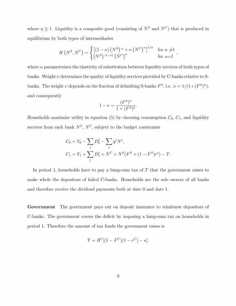
Dynamic responses The lower volatility of prices and quantities in the economies with
higher capital requirements can be seen clearly in figure (4).
35

Quarters5 10 15 20 25
% r
el. Y
sho
ck
0
0.2
0.4
C
Quarters5 10 15 20 25
% r
el. Y
sho
ck
0
2
4
6
H
Quarters5 10 15 20 25
% r
el. Y
sho
ck
0
2
4
AS
Quarters5 10 15 20 25
% r
el. Y
sho
ck-10
0
10
20
30
p
θ = 10%θ = 15%θ = 20%
Figure 4: Impulse responses for different levels of θ
Top left: Consumption, Top right: Utility from liquidity services, Bottom left: Share ofS-banks, Bottom right: Price of Z-asset.
The dynamic responses of consumption and the price of the intermediated asset to an
aggregate income and payoff shock decline in amplitude for higher levels of θ. The responses
of all four variables shown in the figure are less persistent. For low values of θ, the shadow
bank share is procyclical. For levels of θ that are high enough to make both types of banks
safe and hence their liquidity services equally valuable, the asset share hardly responds at
all to aggregate shocks. In addition, the cyclicality reverses, and the shadow bank share now
becomes slightly countercyclical.
36

4 Conclusion
This paper proposes a novel model to study the consequences of higher bank capital re-
quirements for the economy. The optimal level of capital regulation trades-off a reduction in
liquidity services against an increase in the safety of the banking system and consumption.
Increasing the capital requirement for regulated banks leads to more intermediation activity
by the shadow banking system and thus a higher valuation for the intermediated asset be-
cause households’ substitute shadow bank liquidity for commercial bank liquidity. This effect
is non-monotonic as shadow banks’ endogenous borrowing constraint restricts their ability
to provide liquidity services. Moreover, a higher capital requirement makes both bank types
safer: they affect commercial banks directly through a mandated reduction in leverage while
they make shadow banks indirectly safer through their effect on the intermediated asset
valuation.
37
References
Acharya, V. V., P. Schnabl, and G. Suarez (2013): “Securitization without risk
transfer,” Journal of Financial economics, 107, 515–536.
Adrian, T. and A. B. Ashcraft (2012): “Shadow banking: a review of the literature,”
FRB of New York Staff Report.
Adrian, T. and H. S. Shin (2010): “Liquidity and leverage,” Journal of financial inter-
mediation, 19, 418–437.
Azar, J., J.-F. Kagy, and M. C. Schmalz (2014): “Can changes in the cost of carry
explain the dynamics of corporate ”cash” holdings?” Tech. rep., Working paper, University
of Michigan.
Bernanke, B. S. (2005): “The global saving glut and the US current account deficit,”
Tech. rep.
Caballero, R. J. and A. Krishnamurthy (2009): “Global Imbalances and Financial
Fragility,” American Economic Review, 99, 584–88.
Chernenko, S. and A. Sunderam (2014): “Frictions in Shadow Banking: Evidence from
the Lending Behavior of Money Market Mutual Funds,” Review of Financial Studies, 27,
1717–1750.
Christiano, L., R. Motto, and M. Rostagno (2010): “Financial Factors in economic
Fluctuations,” .
Diamond, D. W. and P. H. Dybvig (1983): “Bank Runs, Deposit Insurance, and Liq-
uidity,” Journal of Political Economy, 91, 401–419.
38

Diamond, D. W. and R. G. Rajan (2001): “Liquidity Risk, Liquidity Creation, and
Financial Fragility: A Theory of Banking,” Journal of Political Economy, 109, 287–327.
Feenstra, R. C. (1986): “Functional Equivalence between Liquidity Costs and the Utility
of Money,” Journal of Monetary Economics, 17, 271–291.
Flannery, M. J. and S. M. Sorescu (1996): “Evidence of bank market discipline in
subordinated debenture yields: 1983–1991,” The Journal of Finance, 51, 1347–1377.
Freixas, X. and J.-c. Rochet (1998): Microeconomics of Banking, MIT Press, Cam-
bridge, Massachusetts.
Gandhi, P. and H. Lustig (2013): “Size anomalies in US bank stock returns,” The Journal
of Finance.
Gennaioli, N., A. Shleifer, and R. W. Vishny (2013): “A model of shadow banking,”
The Journal of Finance, 68, 1331–1363.
Gertler, M. and P. Karadi (2011): “A model of unconventional monetary policy,”
Journal of monetary Economics, 58, 17–34.
Gertler, M. and N. Kiyotaki (2010): “Financial intermediation and credit policy in
business cycle analysis,” Handbook of monetary economics, 3, 547–599.
Gertler, M., N. Kiyotaki, and A. Prespitino (2015): “Wholesale Banking and Bank
Runs in Macroeconomic Modelling of Financial Crises,” .
Gomes, J., U. Jermann, and L. Schmid (2014): “Sticky leverage,” .
Goodhart, C. A., A. K. Kashyap, D. P. Tsomocos, and A. P. Vardoulakis (2012):
“Financial regulation in general equilibrium,” Tech. rep., National Bureau of Economic
Research.
39
Gorton, G., S. Lewellen, and A. Metrick (2012): “The Safe-Asset Share,” The
American Economic Review, 102, 101–106.
Gorton, G. and G. Pennacchi (1990): “Financial Intermediaries and Liqduity Creation,”
The Journal of Finance, 45, 49–71.
Gourinchas, P.-O. and O. Jeanne (2012): “Global safe assets,” .
Gu, C., F. Mattesini, C. Monnet, and R. Wright (2013): “Banking: A new mone-
tarist approach,” The Review of Economic Studies, 80, 636–662.
Kelly, B. T., H. Lustig, and S. Van Nieuwerburgh (2011): “Too-systemic-to-fail:
What option markets imply about sector-wide government guarantees,” Tech. rep., Na-
tional Bureau of Economic Research.
Krishnamurthy, A. and A. Vissing-Jorgensen (2012): “The aggregate demand for
treasury debt,” Journal of Political Economy, 120, 233–267.
——— (2013): “Short-term debt and financial crises: What we can learn from US Treasury
supply,” unpublished, Northwestern University, May.
Meeks, R., B. Nelson, and P. Alessandri (2013): “Shadow banks and macroeconomic
instability,” Bank of Italy Temi di Discussione (Working Paper) No, 939.
Moreira, A. and A. Savov (2014): “The macroeconomics of shadow banking,” Tech.
rep., National Bureau of Economic Research.
Plantin, G. (2014): “Shadow banking and bank capital regulation,” Review of Financial
Studies, hhu055.
Poterba, J. M. and J. J. Rotemberg (1986): “Money in the Utility Function: An
Empirical Implementation,” .
40

Pozsar, Z. (2013): “Institutional cash pools and the Triffin dilemma of the US banking
system,” Financial Markets, Institutions & Instruments, 22, 283–318.
Pozsar, Z., T. Adrian, A. Ashcraft, and H. Boesky (2012): “Shadow Banking,”
Tech. rep., Federal Reserve Bank of New York.
Sidrauski, M. (1967): “Inflation and Economic Growth,” Journal of Political Economy,
75, 796–810.
Sunderam, A. (2014): “Money creation and the shadow banking system,” Review of Fi-
nancial Studies.
41
A Appendix
A.1 Two-period model
Preliminaries Since ρji is uniformly distributed, the probability that bank i with assets
Aji and debt Bj
i stays in business is given by the probability that ρji ≤ Z − Bji
Aji
, i.e.
F jρ
(Z − Bj
i
Aji
)=Z − bji − ρj
ρj − ρj. (21)
Furthermore, ρ−j is the expected value of ρji conditional on j−bank’s survival and a real-
ization of the random variable Z:
ρ−j = Eρ[ρj | ρj < Z − bj] =1
2
(Z − bj + ρj
). (22)
The expected value of ρ conditional on j−bank’s failure is
ρ+j = Eρ[ρj | ρj > Z − bj] =1
2
(Z − bj + ρj
). (23)
First-order conditions with respect to Aj The first-order condition for holdings of the
intermediated asset for both types of banks is
vj(bj) = 0,
which implies
qjbj − p0 = E0
[M(F jρ (Z − bS − ρ−j )
)]using the expressions for vj(bj) defined in equations (4) and (2) for j = C, S, respectively.
We can now substitute the expressions for F jρ given in equation (21) and for ρ−j given in
equation (22) into the condition above, which yields
qjbj − p0 = E0
[M
2(ρj − ρj)
(Z − bj − ρj
)2].
42

Using once more the definition of F jρ this becomes
qjbj − p0 = E0
[M(ρj − ρj)
2
(F jρ
)2].
Recognizing that the standard deviation of a uniform random variable with support [ρj, ρj]
is given by
σj =ρj − ρj√12
and plugging in gives the result in equations (10) and (11), respectively.
First-order condition for bC Starting with the definition of vC(bC) in equation (4), and
substituting the expressions for FCρ and ρ−C given in equations (21) and (22), we get
vC(bC) = (qC − κ)bC − p0 − E0
[M
2(ρC − ρC)
(Z − bC − ρC
)2].
Taking the derivative with respect to bC (including the leverage constraint bC ≤ (1 − θ)p0)
then yields
qC − κ = λC + E0
[M
(Z − bC − ρj
ρj − ρj
)],
which gives the result in equation (12).
First-order condition for bS To derive the FOC of the S-bank, it is helpful to first rewrite
several expressions. As for the C-bank, we can write the continuation value as
F S(Z − bS − ρ−S ) =1
2(ρS − ρS)(Z − bS − ρS)2.
Furthermore, noting that Z − ρ+S = 12(Z + bS − ρS), we get for the recovery value on the
bonds of bankrupt S-banks
(1− F S
)rS =
1− ξS2(ρS − ρS)
(bS)2 − (Z − ρS
)2bS
.
43

Using these expressions, we can rewrite HH’s FOC for NS (see equation 8) as
qS = E0
{M1
1
(ρS − ρS)
[Z − bS − ρS + 0.5 (1− ξS)
(bS)2 − (Z − ρS
)2bS
+MRSS
]}.
Taking the derivative of this equation with respect to bS
∂qS(bS)
∂bS= −E0
{M1
(ξS
ρS − ρS+(1− F S
) rSbS
)}. (24)
We can now derive the S-bank’s FOC with respect to its leverage ratio bS
qS + bS∂qS(bS)
∂bS= E0
[M1
Z − bS − ρS
ρS − ρS
].
Plugging in from equation (24), and noting that the last term on the right-hand side equal
the survival probability F S
qS − E0M1
[bSξS
ρS − ρS+ (1− F S)rS
]= E0M1F
S,
which can be rearranged to yield
qS − E0M1
[F S + (1− F S)rS
]= E0M1
1
ρS − ρSξSb
S.
Using the HH’s FOC for shadow bank debt (8), we can substitute for the difference on the
LHS
E0
[M1 (1− ν)
U1
U2
(H
NS
)1−α]= E0
[M1
1
ρS − ρSξSb
S
],
and solve for bS, which yields the expression in equation (14).
Equations and Solution Method The equilibrium of the economy needs to be computed
numerically. The equilibrium can be reduced to a system of four nonlinear equations in four
unknowns. We numerically find a unique solution for every parameter combination we have
tried. The four variables are (p0, AS, C1, b
S). Using the variables, we can first compute the
C-bank leverage ratio as
bC = (1− θ)p0
44

Using the market clearing conditions NS = bSAS, NC = ACbC(1− (1− FC)(1− rC) + κ
)and AC = 1− AS, we can get the two bond prices (qS, qC) from the HH FOCs for deposits.
Then the four equations are
p0 = (qC − κ)bC + E0
(M1
1
4σ2√3(Z − bC − ρC)2
)p0 = qSbS + E0
(M1
1
4σ2√3(Z − bS − ρS)2
)C1 = Y1 +
∑j
Dj1 +NC +NS(F S + (1− F S)rs)
bS = E0
(√12σSξS
(1− ν)
(1− ψ (H/C1)
1−η
ψ (H/C1) −η
)(H
NS
)1−α).
45


