
Finding the Best System — Ranking andSelection Methods
Dave Goldsman
School of ISyEGeorgia Institute of Technology
Atlanta, GA, [email protected]
September 14, 2016
1 / 80

Outline1 Introduction
Classical Confidence IntervalsRanking and Selection
2 Find the Normal Distribution with the Largest MeanSingle-Stage ProcedureTwo-Stage ProcedureSequential Procedure
3 Find the Bernoulli Distrn with the Largest Success ProbSingle-Stage ProcedureSequential Procedure
4 Find the Most Probable Multinomial CellSingle-Stage ProcedureCurtailed ProcedureSequential ProcedureNonparametric Applications
2 / 80

Introduction
Statistics / Simulation experiments are typically performed to analyzeor compare a “small” number of systems, say ≤ 200.
The appropriate method depends on the type of comparison desiredand properties of the output data.
If we analyze one system, we could use traditional confidenceintervals (CIs) based on the normal or t-distributions from our babystatistics class.
If we compare two systems, we could again use CIs from baby stats— maybe even clever ones based on paired observations.
If we compare > 2 systems, we may want to use ranking andselection techniques.
3 / 80

Introduction
Classical Confidence Intervals
Confidence Intervals
One-Sample Case: If we are interested in obtaining a two-sided100(1− α)% CI for the unknown mean µ of independent andidentically distributed (i.i.d.) normal data X1, X2, . . . , Xn withunknown variance σ2, then one would use the well-knownt-distribution based CI, which I’ll quickly derive for your viewingpleasure.
First of all, recall that
The sample mean Xn ≡∑n
i=1Xi/n ∼ Nor(µ, σ2/n).
The sample varianceS2X ≡
∑ni=1(Xi − Xn)2/(n− 1) ∼ σ2χ2(n− 1)/(n− 1).
Xn and S2X are independent.
4 / 80

Introduction
Classical Confidence Intervals
With these facts in mind, we have
T =Xn − µ√S2X/n
=
Xn−µ√σ2/n√S2X/σ
2∼ Nor(0, 1)√
χ2(n−1)n−1
∼ t(n− 1).
Letting the notation tγ,ν denotes the 1− γ quantile of a t-distributionwith ν degrees of freedom, we have
1− α = P (−tα/2,n−1 ≤ T ≤ tα/2,n−1)
= P
(−tα/2,n−1 ≤
Xn − µ√S2X/n
≤ tα/2,n−1
)= P
(Xn − tα/2,n−1SX/
√n ≤ µ ≤ Xn + tα/2,n−1SX/
√n).
So we have the following 100(1− α)% CI for µ,
µ ∈ Xn ± tα/2,n−1SX/√n.
5 / 80

Introduction
Classical Confidence Intervals
Two-Sample Case: Suppose that X1, X2, . . . , Xn are i.i.d.Nor(µX , σ2
X) and Y1, Y2, . . . , Ym are i.i.d. Nor(µY , σ2Y ).
A CI for the difference between µX − µY can be carried out by any ofthe following methods, all of which are readily available in anystandard statistics textbook.
pooled CI (use when σ2X and σ2
Y are equal but unknown)
approximate CI (use when σ2X and σ2
Y are unequal and unknown)
paired CI (use when Cov(Xi, Yi) > 0)
In what follows, Xn, Ym, S2X , and S2
Y are the obvious sample meansand variances of the X’s and Y ’s.
6 / 80

Introduction
Classical Confidence Intervals
Pooled CI: If the X’s and Y ’s are independent but with common,unknown variance, then the usual CI for the difference in means is
µX − µY ∈ Xn − Ym ± tα/2,n+m−2 SP
√1
n+
1
m,
where
S2P ≡
(n− 1)S2X + (m− 1)S2
Y
n+m− 2
is the pooled variance estimator for σ2.
7 / 80

Introduction
Classical Confidence Intervals
Approximate CI: If the X’s and Y ’s are independent but with arbitraryunknown variances, then the usual CI for the difference in means is
µX − µY ∈ X − Y ± tα/2,ν
√S2X
n+S2Y
m.
This CI requires an approximation.
t? ≡ X − Y − (µX − µY )√S2Xn +
S2Ym
≈ t(ν),
where the approximate degrees of freedom is given by
ν ≡
(S2Xn +
S2Ym
)2
(S2X/n)2
n+1 +(S2
Y /m)2
m+1
− 2.
8 / 80

Introduction
Classical Confidence Intervals
Example: Two normal populations. Let’s get a 95% CI for µX − µY .Suppose it turns out that
n = 25 X = 100 S2X = 400
m = 16 Y = 80 S2Y = 100
You can tell from S2X and S2
Y that there’s no way that the two var’sare equal. So we’ll have to use the approximation method, with d.f.
ν =
(40025 + 100
16
)2
(400/25)2
26 + (100/16)2
17
− 2 = 38.77 ≈ 38,
where we round d.f. down to be conservative (i.e., slightly longer CI).
Noting that tα/2,ν = t0.025,38 = 2.02, we obtain
µX − µY ∈ 20± 2.02√
22.25 = 20± 9.53. 2
9 / 80

Introduction
Classical Confidence Intervals
Paired CI: Again consider two competing normal pop’ns withunknown means µX and µY . Suppose we collect observations fromthe two pop’ns in pairs.
Different pairs are independent, but the two obs’ns within the samepair may not be indep.
indep
Pair 1 : (X1, Y1)
Pair 2 : (X2, Y2)...
...
Pair n : (Xn, Yn)︸ ︷︷ ︸not indep
Example: Think sets of twins. One twin takes a new drug, the othertakes a placebo.
10 / 80
Introduction
Classical Confidence Intervals
Idea: By setting up such experiments, we hope to be able to capturethe difference between the two normal pop’ns more precisely, sincewe’re using the pairs to eliminate extraneous noise.
Here’s the set-up. Take n pairs of observations:
X1, X2, . . . , Xniid∼ Nor(µX , σ2
X)
Y1, Y2, . . . , Yniid∼ Nor(µY , σ2
Y ).
(Technical assumption: All Xi’s and Yj’s are jointly normal.)
We assume that the variances σ2X and σ2
Y are unknown and possiblyunequal.
Further, pair i is indep of pair j (between pairs), but Xi may not beindep of Yi (within a pair).
11 / 80

Introduction
Classical Confidence Intervals
Define the pair-wise differences, Di ≡ Xi − Yi, i = 1, 2, . . . , n.
Then D1, D2, . . . , Dniid∼ Nor(µD, σ2
D), where µD ≡ µX − µY(which is what we want the CI for), and
σ2D ≡ σ2
X + σ2Y − 2Cov(Xi, Yi).
Now the problem reduces to the old Nor(µ, σ2) case with unknown µand σ2. So let’s calculate the sample mean and variance as before.
D ≡ 1
n
n∑i=1
Di ∼ Nor(µD, σ2D/n)
S2D ≡ 1
n− 1
n∑i=1
(Di − D)2 ∼σ2Dχ
2(n− 1)
n− 1.
Just like before, get the CI
µD ∈ D ± tα/2,n−1
√S2D/n.
12 / 80

Introduction
Classical Confidence Intervals
Example: Times for people to parallel park two cars (assume normal).
Person Park Honda Park Cadillac Difference
1 10 20 −10
2 25 40 −15
3 5 5 0
4 20 35 −15
5 15 20 −5
Clearly, the people are indep, but the times for the same individual topark the two cars may not be indep.
We have n = 5, D = −9, S2D = 42.5. Thus, the 90% two-sided CI is
µD ∈ −9± 2.13√
42.5/5 = −9± 6.21. 2
13 / 80

Introduction
Classical Confidence Intervals
So why didn’t we just use the “usual” CI for the difference of twomeans? Namely,
µX − µY ∈ X − Y ± tα/2,ν
√S2X
n+S2Y
m.
Main reason: This CI requires that the X’s must be indep of the Y ’s.(Recall that the paired-t method allows Xi and Yi to be dependent.)
Good thing: The approx d.f. ν from the “usual” method wouldprobably be larger than the d.f. n− 1 from the paired-t method. Thiswould make the CI smaller.
Bad thing: You’d introduce much more noise into the system by usingthe “usual” method. This could make the CI much larger.
14 / 80

Introduction
Classical Confidence Intervals
Example: Back to the car example.
A guy parks Same guy Different guy
Honda Xi parks Caddy parks Caddy Yi10 20 30
25 40 15
5 5 40
20 35 10
15 20 25
Just concentrate on the Xi and Yi columns. (The middle column isfrom the last example for comparison purposes.)
The Xi’s and Yj’s have the same sample averages as before, but nowthere’s more natural variation since we’re using 10 different people.
15 / 80

Introduction
Classical Confidence Intervals
Now all of the Xi’s are indep of all of the Yi’s.
X = 15, Y = 24, S2X = 62.5, S2
Y = 142.5.
Then we have
ν =
(S2Xn +
S2Yn
)2
(S2X/n)2
n+1 +(S2
Y /n)2
n+1
− 2 ≈ 8.
This gives us the following 90% CI,
µX − µY ∈ X − Y ± t0.05,8
√S2X
n+S2Y
n= −9± 11.91.
This CI is wider than the paired-t version, even though we have mored.f. here. 2
Moral: Use paired-t when you can.16 / 80

Introduction
Ranking and Selection
Ranking and Selection
For > 2 systems, we could use methods such as simultaneous CIs andANOVA. But those methods don’t tell us much except that “at leastone of the systems is different than the others”, which is no surprise.
And what measures do you use to compare different systems?
* Which has the biggest mean?
* The smallest variance?
* The highest probability of yielding a success?
* The lowest risk?
* A combination of criteria?
17 / 80

Introduction
Ranking and Selection
Remainder of this module: We present ranking & selectionprocedures to find the best system with respect to one parameter.
Examples:
Great Expectations: Which of 10 fertilizers produces the largest meancrop yield? (Normal)
Great Expectorants: Find the pain reliever that has the highestprobability of giving relief for a cough. (Binomial)
Great Ex-Patriots: Who is the most-popular former New Englandfootball player? (Multinomial)
18 / 80

Introduction
Ranking and Selection
R&S selects the best system, or a subset of systems that includes thebest.
Guarantee a probability of a correct selection.
Multiple Comparisons Procedures (MCPs) add in certainconfidence intervals.
R&S is relevant in simulation:
Normally distributed data by batching.
Independence by controlling random numbers.
Multiple-stage sampling by retaining the seeds.
19 / 80

Find the Normal Distribution with the Largest Mean
Outline1 Introduction
Classical Confidence IntervalsRanking and Selection
2 Find the Normal Distribution with the Largest MeanSingle-Stage ProcedureTwo-Stage ProcedureSequential Procedure
3 Find the Bernoulli Distrn with the Largest Success ProbSingle-Stage ProcedureSequential Procedure
4 Find the Most Probable Multinomial CellSingle-Stage ProcedureCurtailed ProcedureSequential ProcedureNonparametric Applications
20 / 80

Find the Normal Distribution with the Largest Mean
We give procedures for selecting that one of k normal distributionshaving the largest mean.
We use the indifference-zone approach.
Assumptions: Independent Yi1, Yi2, . . . (1 ≤ i ≤ k) are taken fromk ≥ 2 normal populations Π1, . . . ,Πk. Here Πi has unknown mean µiand known or unknown variance σ2
i .
Denote the vector of means by µ = (µ1, . . . , µk) and the vector ofvariances by σ2 = (σ2
1, . . . , σ2k).
The ordered (but unknown) µi’s are µ[1] ≤ · · · ≤ µ[k].
The system having the largest mean µ[k] is the “best.”
21 / 80

Find the Normal Distribution with the Largest Mean
Goal: To select the population associated with mean µ[k].
A correct selection (CS) is made if the Goal is achieved.
Indifference-Zone Probability Requirement: For specified constants(P ?, δ?) with δ? > 0 and 1/k < P ? < 1, we require
P{CS} ≥ P ? whenever µ[k] − µ[k−1] ≥ δ?. (1)
The constant δ? can be thought of as the “smallest difference worthdetecting.”
The probability in (1) depends on the differences µi − µj , the samplesize n, and σ2.
22 / 80
Find the Normal Distribution with the Largest Mean
Parameter configurations µ satisfying µ[k] − µ[k−1] ≥ δ? are in thepreference-zone for a correct selection.
Configurations satisfying µ[k] − µ[k−1] < δ? are in theindifference-zone.
Any procedure that guarantees (1) is said to be employing theindifference-zone approach.
There are 100’s of such procedures. Highlights:
* Single-Stage Procedure (Bechhofer 1954)
* Two-Stage Procedure (Rinott 1979)
* Sequential Procedure (Kim and Nelson 2001)
23 / 80

Find the Normal Distribution with the Largest Mean
Single-Stage Procedure
Single-Stage Procedure NB (Bechhofer 1954)
This procedure takes all necessary observations and makes theselection decision at once (in a single stage).
Assumes pop’ns have common known variance.
For the given k and specified (P ?, δ?/σ), determine sample size n(usually from a table).
Take a random sample of n observations Yij (1 ≤ j ≤ n) in a singlestage from Πi (1 ≤ i ≤ k).
Calculate the k sample means, Yi =∑n
j=1 Yij/n (1 ≤ i ≤ k).
Select the pop’n that yielded the largest sample mean,Y[k] = max{Y1, . . . , Yk}, as the one associated with µ[k].
Very intuitive — all you have to do is figure out n.24 / 80

Find the Normal Distribution with the Largest Mean
Single-Stage Procedure
δ?/σ
k P ? 0.1 0.2 0.3 0.4 0.5 0.6 0.7 0.8 0.9 1.0
0.75 91 23 11 6 4 3 2 2 2 1
2 0.90 329 83 37 21 14 10 7 6 5 4
0.95 542 136 61 34 22 16 12 9 7 6
0.99 1083 271 121 68 44 31 23 17 14 11
0.75 206 52 23 13 9 6 5 4 3 3
3 0.90 498 125 56 32 20 14 11 8 7 5
0.95 735 184 82 46 30 21 15 12 10 8
0.99 1309 328 146 82 53 37 27 21 17 14
0.75 283 71 32 18 12 8 6 5 4 3
4 0.90 602 151 67 38 25 17 13 10 8 7
0.95 851 213 95 54 35 24 18 14 11 9
0.99 1442 361 161 91 58 41 30 23 18 15
Common Sample Size n per Pop’n Required by NB
25 / 80

Find the Normal Distribution with the Largest Mean
Single-Stage Procedure
Remark: Don’t really need the above table. You can directly calculate
n =
⌈2(σZ
(1−P ?)k−1,1/2/δ
?)2⌉,
where d·e rounds up, and the constant Z(1−P ?)k−1,1/2 is an upper
equicoordinate point of a certain multivariate normal distribution.
The value of n satisfies (1) for any µ such that
µ[1] = µ[k−1] = µ[k] − δ?. (2)
Configuration (2) is the slippage configuration (since µ[k] is largerthan the other µi’s by a fixed amount). It turns out that for ProcedureNB, (2) is also the least-favorable (LF) configuration because, forfixed n, it minimizes the P{CS} among all µ in the preference-zone.
26 / 80

Find the Normal Distribution with the Largest Mean
Single-Stage Procedure
How to calculate n yourself (without multivariate normal tables).Assume without loss of generality that Πk has the largest µi. Then set
P ? = P{CS |LF} = P{Yi < Yk, i = 1, . . . , k − 1 |LF}
= P
{Yi − µk√σ2/n
<Yk − µk√σ2/n
, i = 1, . . . , k − 1
∣∣∣∣LF
}
=
∫RP
{Yi − µk√σ2/n
< x, i = 1, . . . , k − 1
∣∣∣∣LF
}φ(x) dx
=
∫RP
{Yi − µi√σ2/n
< x+
√nδ?
σ, i = 1, . . . , k − 1
}φ(x) dx
=
∫R
Φk−1
(x+
√nδ?
σ
)φ(x) dx =
∫R
Φk−1(x+ h)φ(x) dx,
where φ(·) and Φ(·) denote the standard normal p.d.f. and c.d.f. Nowsolve numerically for h, and then set n = d(hσ/δ?)2e.
27 / 80

Find the Normal Distribution with the Largest Mean
Single-Stage Procedure
Example: Suppose k = 4 and we want to detect a difference in meansas small as 0.2 standard deviations with P{CS} ≥ 0.99. The table forNB calls for n = 361 observations per pop’n.
If, after taking n = 361 obns, we find that Y1 = 13.2, Y2 = 9.8,Y3 = 16.1, and Y4 = 12.1, then we select pop’n 3 as the best.
Note that increasing δ? and/or decreasing P ? requires a smaller n. Forexample, when δ?/σ = 0.6 and P ? = 0.95, NB requires only n = 24observations per pop’n. 2
Robustness of Procedure: How does NB do under different types ofviolations of the underlying assumptions on which it’s based?
Lack of normality — not so bad.
Different variances — sometimes a big problem.
Dependent data — usually a nasty problem (e.g., in simulations).28 / 80

Find the Normal Distribution with the Largest Mean
Two-Stage Procedure
Two-Stage Procedure NR (Rinott 1979)
Assumes pop’ns have unknown and unequal variances. Takes a firststage of observations to estimate the variances of each system, andthen uses those estimates to determine how many observations to takein the second stage — the higher the variance estimate, the moreobservations needed.
For the given k, specify (P ?, δ?), and a common first-stage samplesize n0 ≥ 2.
Look up the constant g(P ?, n0, k) in an appropriate table or (if youhave the urge) solve the following equation for g:∫ ∞
0
∫ ∞0
Φk−1
(g
(n0 − 1)( 1x + 1
y )
)f(x)f(y) dx dy = P ?,
where f(·) is the χ2(n0 − 1) p.d.f.29 / 80

Find the Normal Distribution with the Largest Mean
Two-Stage Procedure
Take an i.i.d. sample Yi1, Yi2, . . . , Yin0 from each of the k scenariossimulated independently.
Calculate the first-stage sample means and variances,
Yi(n0) =1
n0
n0∑j=1
Yij and S2i =
∑n0j=1
(Yij − Yi(n0)
)2n0 − 1
,
and then the final sample sizes
Ni = max{n0,⌈(gSi/δ
?)2⌉}, i = 1, 2, . . . , k.
Take Ni − n0 additional i.i.d. observations from scenario i,independently of the first-stage sample and the other scenarios, fori = 1, 2, . . . , k.
30 / 80

Find the Normal Distribution with the Largest Mean
Two-Stage Procedure
Compute overall sample means ¯Yi = 1Ni
∑Nij=1 Yij , ∀i.
Select the scenario with the largest ¯Yi as best.
Bonus: Simultaneously form MCP confidence intervals
µi−maxj 6=i
µj ∈
[−(
¯Yi −maxj 6=i
¯Yj − δ?)−
,
(¯Yi −max
j 6=i¯Yj + δ?
)+]
∀i, where (a)+ ≡ max{0, a} and −(b)− ≡ min{0, b}.
31 / 80

Find the Normal Distribution with the Largest Mean
Two-Stage Procedure
k
P ? n0 2 3 4 5 6 7
9 2.656 3.226 3.550 3.776 3.950 4.09110 2.614 3.166 3.476 3.693 3.859 3.99311 2.582 3.119 3.420 3.629 3.789 3.91812 2.556 3.082 3.376 3.579 3.734 3.86013 2.534 3.052 3.340 3.539 3.690 3.81214 2.517 3.027 3.310 3.505 3.654 3.77315 2.502 3.006 3.285 3.477 3.623 3.741
0.95 16 2.489 2.988 3.264 3.453 3.597 3.71317 2.478 2.973 3.246 3.433 3.575 3.68918 2.468 2.959 3.230 3.415 3.556 3.66919 2.460 2.948 3.216 3.399 3.539 3.65020 2.452 2.937 3.203 3.385 3.523 3.63430 2.407 2.874 3.129 3.303 3.434 3.53940 2.386 2.845 3.094 3.264 3.392 3.49550 2.373 2.828 3.074 3.242 3.368 3.469
g Constant Required by NR
32 / 80

Find the Normal Distribution with the Largest Mean
Two-Stage Procedure
Example: A Simulation Study of Airline Reservation Systems
Consider k = 4 different airline reservation systems.
Objective: Find the system with the largest expected time to failure(E[TTF]). Let µi denote the E[TTF] for system i.
From past experience we know that the E[TTF]’s are roughly 100,000minutes (about 70 days) for all four systems.
Goal: Select the best system with probability at least P ? = 0.90 if thedifference in the expected failure times for the best and second bestsystems is ≥ δ? = 3000 minutes (about two days).
The competing systems are sufficiently complicated that computersimulation is required to analyze their behavior.
33 / 80
Find the Normal Distribution with the Largest Mean
Two-Stage Procedure
Let Tij (1 ≤ i ≤ 4, j ≥ 1) denote the observed time to failure fromthe jth independent simulation replication of system i.
Application of the Rinott procedure NR requires i.i.d. normalobservations from each system.
If each simulation replication is initialized from a particular systemunder the same operating conditions, but with independent randomnumber seeds, the resulting Ti1, Ti2, . . . will be i.i.d. for each system.
However, the Tij aren’t normal — in fact, they’re skewed right.
34 / 80

Find the Normal Distribution with the Largest Mean
Two-Stage Procedure
Instead of using the raw Tij in NR, apply the procedure to theso-called macroreplication estimators of the µi.
These estimators group the {Tij :j ≥ 1} into disjoint batches and usethe batch averages as the “data” to which NR is applied.
Fix a number m of simulation replications that comprise eachmacroreplication (that is, m is the batch size) and let
Yij ≡1
m
m∑k=1
Ti,(j−1)m+k, 1 ≤ i ≤ 4, 1 ≤ j ≤ bi,
where bi is the number of macroreplications to be taken from system i.
35 / 80

Find the Normal Distribution with the Largest Mean
Two-Stage Procedure
The macroreplication estimators from the ith system,Yi1, Yi2, . . . , Yibi , are i.i.d. with expectation µi.
If m is sufficiently large, say at least 20, then the CLT yieldsapproximate normality for each Yij .
No assumptions on the variances of the macroreplications.
To apply NR, first conduct a pilot study to serve as the first stage ofthe procedure. Each system was run for n0 = 20 macroreplicationswith each macroreplication consisting of the averages of m = 20simulations of the system.
Rinott table with k = 4 and P ? = 0.90 gives g = 2.720.
The total sample sizes Ni are computed for each system and aredisplayed in the summary table.
36 / 80

Find the Normal Distribution with the Largest Mean
Two-Stage Procedure
i 1 2 3 4
Yi(n0) 108286 107686 96167 89747
Si 29157 24289 25319 20810
Ni 699 485 527 356¯Yi 110816 106411 99093 86568
std. error 872 1046 894 985
Summary of Airline Rez Example
37 / 80

Find the Normal Distribution with the Largest Mean
Two-Stage Procedure
E.g., System 2 requires an additional N2 − 20 = 465macroreplications in the second stage (each macroreplication againbeing the average of m = 20 system simulations).
In all, a total of about 40,000 simulations of the four systems wererequired to implement procedure NR. The combined sample meansfor each system are listed in row 4 of the summary table.
Clearly establish System 1 as having the largest E[TTF]. 2
38 / 80
Find the Normal Distribution with the Largest Mean
Sequential Procedure
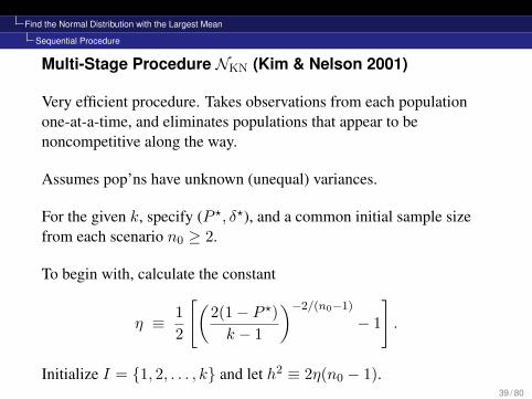
Multi-Stage Procedure NKN (Kim & Nelson 2001)
Very efficient procedure. Takes observations from each populationone-at-a-time, and eliminates populations that appear to benoncompetitive along the way.
Assumes pop’ns have unknown (unequal) variances.
For the given k, specify (P ?, δ?), and a common initial sample sizefrom each scenario n0 ≥ 2.
To begin with, calculate the constant
η ≡ 1
2
[(2(1− P ?)k − 1
)−2/(n0−1)
− 1
].
Initialize I = {1, 2, . . . , k} and let h2 ≡ 2η(n0 − 1).39 / 80

Find the Normal Distribution with the Largest Mean
Sequential Procedure
Take an initial random sample of n0 ≥ 2 observations Yij(1 ≤ j ≤ n0) from population i (1 ≤ i ≤ k).
For population i, compute the sample mean based on the n0
observations, Yi(n0) =∑n0
j=1 Yij/n0 (1 ≤ i ≤ k).
For all i 6= `, compute the sample variance of the difference betweenpopulations i and `,
S2i` =
1
n0 − 1
n0∑j=1
(Yij − Y`j − [Yi(n0)− Y`(n0)]
)2.
For all i 6= `, set Ni` =⌊h2S2
i`/(δ?)2⌋
and then Ni = max`6=iNi`.
40 / 80

Find the Normal Distribution with the Largest Mean
Sequential Procedure
If n0 > maxiNi, stop and select the population with the largestsample mean Yi(n0) as one having the largest mean. Otherwise, setthe sequential counter r = n0 and go to the Screening phase of theprocedure.
Screening: Set Iold = I and re-set
I = {i : i ∈ Iold and Yi(r) ≥ Y`(r)−Wi`(r),
for all ` ∈ Iold, ` 6= i},
where
Wi`(r) = max
{0,δ?
2r
(h2S2
i`
(δ?)2− r)}
.
Keep those surviving populations that aren’t “too far” from thecurrent leader.
41 / 80

Find the Normal Distribution with the Largest Mean
Sequential Procedure
Stopping Rule: If |I| = 1, then stop and select the treatment withindex in I as having the largest mean.
If |I| > 1, take one additional observation Yi,r+1 from each treatmenti ∈ I .
Increment r = r+ 1 and go to the screening stage if r < maxiNi + 1.
If r = maxiNi + 1, then stop and select the treatment associated withthe largest Yi(r) having index i ∈ I .
42 / 80

Find the Normal Distribution with the Largest Mean
Sequential Procedure
Normal Extensions
Correlation between populations.
Better fully sequential procedures.
Better elimination of pop’ns that aren’t competitive.
Different variance estimators.
43 / 80

Find the Bernoulli Distrn with the Largest Success Prob
Outline1 Introduction
Classical Confidence IntervalsRanking and Selection
2 Find the Normal Distribution with the Largest MeanSingle-Stage ProcedureTwo-Stage ProcedureSequential Procedure
3 Find the Bernoulli Distrn with the Largest Success ProbSingle-Stage ProcedureSequential Procedure
4 Find the Most Probable Multinomial CellSingle-Stage ProcedureCurtailed ProcedureSequential ProcedureNonparametric Applications
44 / 80

Find the Bernoulli Distrn with the Largest Success Prob
Examples:
Which anti-cancer drug is most effective?
Which simulated system is most likely to meet design specs?
There are 100’s of such procedures. Highlights:
Single-Stage Procedure (Sobel and Huyett 1957)
Sequential Procedure (Bechhofer, Kiefer, Sobel 1968)
“Optimal” Procedures (Bechhofer, et al., 1980’s)
Again use the indifference-zone approach.
45 / 80

Find the Bernoulli Distrn with the Largest Success Prob
Single-Stage Procedure
A Single-Stage Procedure (Sobel and Huyett 1957)
We have k competing Bern populations with success parametersp1, p2, . . . , pk. Denote the ordered p’s by p[1] ≤ p[2] ≤ · · · ≤ p[k].
Probability Requirement: For specified constants (P ?,∆?) with1/k < P ? < 1 and 0 < ∆? < 1, we require
P{CS} ≥ P ? whenever p[k] − p[k−1] ≥ ∆?.
The P{CS} depends on the entire vector p and on the number n ofobservations taken from each of the k treatments.
Note that the probability requirement is defined in terms of thedifference p[k] − p[k−1], and we interpret ∆? as the “smallestdifference worth detecting.”
46 / 80

Find the Bernoulli Distrn with the Largest Success Prob
Single-Stage Procedure
Procedure BSH
For the specified (P ?,∆?), find n from a table.
Take a sample of n observations Xij (1 ≤ j ≤ n) in a single stagefrom each population (1 ≤ i ≤ k).
Calculate the k sample sums Yin =∑n
j=1Xij .
Select the treatment that yielded the largest Yin as the one associatedwith p[k]; in the case of ties, randomize.
47 / 80

Find the Bernoulli Distrn with the Largest Success Prob
Single-Stage Procedure
P ?
k ∆? 0.60 0.75 0.80 0.85 0.90 0.95 0.99
0.10 20 52 69 91 125 184 327
0.20 5 13 17 23 31 46 81
3 0.30 3 6 8 10 14 20 35
0.40 2 4 5 6 8 11 20
0.50 2 3 3 4 5 7 12
0.10 34 71 90 114 150 212 360
0.20 9 18 23 29 38 53 89
4 0.30 4 8 10 13 17 23 39
0.40 3 5 6 7 9 13 21
0.50 2 3 4 5 6 8 13
Smallest n for BSH to Guarantee Prob Reqt48 / 80

Find the Bernoulli Distrn with the Largest Success Prob
Single-Stage Procedure
Example: Suppose we want to select the best of k = 4 treatmentswith probability at least P ? = 0.95 whenever p[4] − p[3] ≥ 0.10.
The table shows that we need n = 212 observations.
Suppose that, at the end of sampling, we have Y1,212 = 70,Y2,212 = 145, Y3,212 = 95 and Y4,212 = 102.
Then we select population 2 as the best. 2
49 / 80
Find the Bernoulli Distrn with the Largest Success Prob
Sequential Procedure
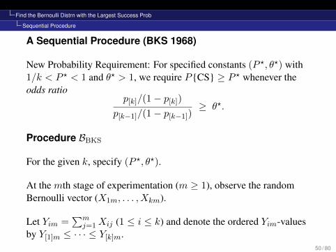
A Sequential Procedure (BKS 1968)
New Probability Requirement: For specified constants (P ?, θ?) with1/k < P ? < 1 and θ? > 1, we require P{CS} ≥ P ? whenever theodds ratio
p[k]/(1− p[k])
p[k−1]/(1− p[k−1])≥ θ?.
Procedure BBKS
For the given k, specify (P ?, θ?).
At the mth stage of experimentation (m ≥ 1), observe the randomBernoulli vector (X1m, . . . , Xkm).
Let Yim =∑m
j=1Xij (1 ≤ i ≤ k) and denote the ordered Yim-valuesby Y[1]m ≤ · · · ≤ Y[k]m.
50 / 80

Find the Bernoulli Distrn with the Largest Success Prob
Sequential Procedure
After the mth stage of experimentation, compute
Zm =
k−1∑i=1
(1/θ?)Y[k]m−Y[i]m .
Stop at the first value of m (call it N ) for which Zm ≤ (1− P ?)/P ?.Note that N is a random variable.
Select the treatment that yielded Y[k]N as the one associated with p[k].
51 / 80
Find the Bernoulli Distrn with the Largest Success Prob
Sequential Procedure
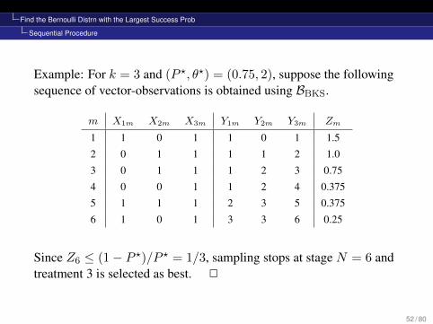
Example: For k = 3 and (P ?, θ?) = (0.75, 2), suppose the followingsequence of vector-observations is obtained using BBKS.
m X1m X2m X3m Y1m Y2m Y3m Zm
1 1 0 1 1 0 1 1.5
2 0 1 1 1 1 2 1.0
3 0 1 1 1 2 3 0.75
4 0 0 1 1 2 4 0.375
5 1 1 1 2 3 5 0.375
6 1 0 1 3 3 6 0.25
Since Z6 ≤ (1− P ?)/P ? = 1/3, sampling stops at stage N = 6 andtreatment 3 is selected as best. 2
52 / 80

Find the Bernoulli Distrn with the Largest Success Prob
Sequential Procedure
Bernoulli Extensions
Correlation between populations.
More-efficient sequential procedures.
Elimination of populations that aren’t competitive.
53 / 80

Find the Most Probable Multinomial Cell
Outline1 Introduction
Classical Confidence IntervalsRanking and Selection
2 Find the Normal Distribution with the Largest MeanSingle-Stage ProcedureTwo-Stage ProcedureSequential Procedure
3 Find the Bernoulli Distrn with the Largest Success ProbSingle-Stage ProcedureSequential Procedure
4 Find the Most Probable Multinomial CellSingle-Stage ProcedureCurtailed ProcedureSequential ProcedureNonparametric Applications
54 / 80

Find the Most Probable Multinomial Cell
Examples:
Who is the most popular political candidate?
Which television show is most watched during a particular timeslot?
Which simulated warehouse configuration is most likely tomaximize throughput?
Yet again, use the indifference-zone approach.
55 / 80

Find the Most Probable Multinomial Cell
Experimental Set-Up:
• k possible outcomes (categories).
• pi is the probability of the ith category.
• n independent replications of the experiment.
• Yi is the number of outcomes falling in category i after the nobservations have been taken.
56 / 80

Find the Most Probable Multinomial Cell
Definition: If the k-variate discrete vector random variableY = (Y1, Y2, . . . , Yk) has the probability mass function
P{Y1 = y1, Y2 = y2, . . . , Yk = yk} =n!∏ki=1 yi!
k∏i=1
pyii ,
then Y has a multinomial distribution with parameters n andp = (p1, . . . , pk), where
∑ki=1 pi = 1 and pi > 0 for all i.
57 / 80

Find the Most Probable Multinomial Cell
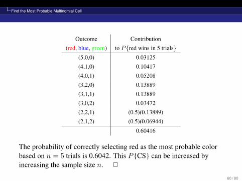
Example: Suppose three of the faces of a fair die are red, two are blue,and one is green, i.e., p = (3/6, 2/6, 1/6).
Toss it n = 5 times. Then the probability of observing exactly threereds, no blues and two greens is
P{Y = (3, 0, 2)} =5!
3!0!2!(3/6)3(2/6)0(1/6)2 = 0.03472. 2
Example (continued): Suppose we did not know the probabilities forred, blue, and green in the previous example and that we want toselect the most probable color.
The selection rule is to choose the color that occurs the mostfrequently during the five trials, using randomization to break ties.
58 / 80

Find the Most Probable Multinomial Cell
Let Y = (Yr, Yb, Yg) denote the number of occurrences of (red, blue,green) in five trials. The probability that we correctly select red isgiven by
P{red wins in 5 trials}= P{Yr > Yb and Yg}+ 0.5P{Yr = Yb, Yr > Yg}
+ 0.5P{Yr > Yb, Yr = Yg}= P{Y = (5, 0, 0), (4, 1, 0), (4, 0, 1), (3, 2, 0), (3, 1, 1), (3, 0, 2)}
+ 0.5P{Y = (2, 2, 1)}+ 0.5P{Y = (2, 1, 2)}.
We can list the outcomes favorable to a correct selection (CS) of red,along with the associated probabilities of these outcomes,randomizing for ties.
59 / 80
Find the Most Probable Multinomial Cell
Outcome Contribution
(red, blue, green) to P{red wins in 5 trials}(5,0,0) 0.03125
(4,1,0) 0.10417
(4,0,1) 0.05208
(3,2,0) 0.13889
(3,1,1) 0.13889
(3,0,2) 0.03472
(2,2,1) (0.5)(0.13889)
(2,1,2) (0.5)(0.06944)
0.60416
The probability of correctly selecting red as the most probable colorbased on n = 5 trials is 0.6042. This P{CS} can be increased byincreasing the sample size n. 2
60 / 80
Find the Most Probable Multinomial Cell
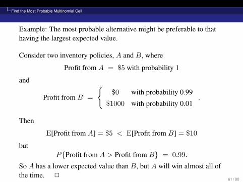
Example: The most probable alternative might be preferable to thathaving the largest expected value.
Consider two inventory policies, A and B, where
Profit from A = $5 with probability 1
and
Profit from B =
{$0 with probability 0.99
$1000 with probability 0.01.
Then
E[Profit from A] = $5 < E[Profit from B] = $10
butP{Profit from A > Profit from B} = 0.99.
So A has a lower expected value than B, but A will win almost all ofthe time. 2
61 / 80

Find the Most Probable Multinomial Cell
Assumptions and Notation
•Xj = (X1j , . . . , Xkj) (j ≥ 1) are independent observations takenfrom a multinomial distribution having k ≥ 2 categories withassociated unknown probabilities p = (p1, . . . , pk).
• Xij = 1 [0] if category i does [does not] occur on the jthobservation.
• The (unknown) ordered pi’s are p[1] ≤ · · · ≤ p[k].
• The category with p[k] is the most probable or best.
• The cumulative sum for category i after m multinomialobservations have been taken is Yim =
∑mj=1Xij .
• The ordered Yim’s are Y[1]m ≤ · · · ≤ Y[k]m.62 / 80

Find the Most Probable Multinomial Cell
Indifference-Zone Procedures
Goal: Select the category associated with p[k].
A correct selection (CS) is made if the Goal is achieved.
Probability Requirement: For specified constants (P ?, θ?) with1/k < P ? < 1 and θ? > 1, we require
P{CS} ≥ P ? whenever p[k]/p[k−1] ≥ θ?. (3)
The probability in (3) depends on the entire vector p and on thenumber n of independent multinomial observations to be taken.
θ? is the “smallest p[k]/p[k−1] ratio worth detecting.”
Now we will consider a number of procedures to guaranteeprobability requirement (3).
63 / 80

Find the Most Probable Multinomial Cell
Single-Stage Procedure
Single-Stage ProcedureMBEM (Bechhofer, Elmaghraby,and Morse 1959):
For the given k, P ? and θ?, find n from the table.
Take n multinomial observationsXj = (X1j , . . . , Xkj) (1 ≤ j ≤ n)in a single stage.
Calculate the ordered sample sums Y[1]n ≤ · · · ≤ Y[k]n. Select thecategory with the largest sample sum, Y[k]n, as the one associated withp[k], randomizing to break ties.
Remark: The n-values are computed so thatMBEM achievesP{CS} ≥ P ? when the cell probabilities p are in the least-favorable(LF) configuration (Kesten and Morse 1959),
p[1] = p[k−1] = 1/(θ? + k − 1) and p[k] = θ?/(θ? + k − 1). (4)
64 / 80

Find the Most Probable Multinomial Cell
Single-Stage Procedure
Example: A soft drink producer wants to find the most popular ofk = 3 proposed cola formulations.
The company will give a taste test to n people.
The sample size n is to be chosen so that P{CS} ≥ 0.95 wheneverthe ratio of the largest to second largest true (but unknown)proportions is at least 1.4.
Entering the table with k = 3, P ? = 0.95, and θ? = 1.4, we find thatn = 186 individuals must be interviewed.
If we find that Y1,186 = 53, Y2,186 = 110, and Y3,186 = 26, then weselect formulation 2 as the best. 2
65 / 80

Find the Most Probable Multinomial Cell
Single-Stage Procedure
k = 2 k = 3 k = 4 k = 5
P ? θ? n n0 n n0 n n0 n n0
2.0 5 5 12 13 20 24 29 341.8 5 7 17 18 29 35 41 50
0.75 1.6 9 9 26 32 46 57 68 861.4 17 19 52 71 92 124 137 1841.2 55 67 181 285 326 495 486 730
2.0 15 15 29 34 43 53 58 711.8 19 27 40 50 61 75 83 104
0.90 1.6 31 41 64 83 98 126 134 1721.4 59 79 126 170 196 274 271 3741.2 199 267 437 670 692 1050 964 1460
2.0 23 27 42 52 61 74 81 981.8 33 35 59 71 87 106 115 142
0.95 1.6 49 59 94 125 139 180 185 2401.4 97 151 186 266 278 380 374 5101.2 327 455 645 960 979 1500 1331 2000
Sample Sizes n forMBEM and Truncation Numbers n0 forMBG to Guarantee (3)
66 / 80
Find the Most Probable Multinomial Cell
Curtailed Procedure
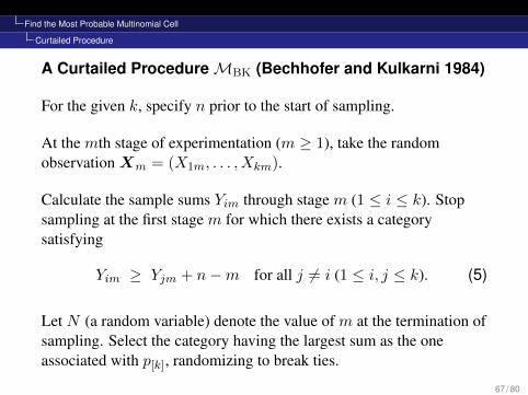
A Curtailed ProcedureMBK (Bechhofer and Kulkarni 1984)
For the given k, specify n prior to the start of sampling.
At the mth stage of experimentation (m ≥ 1), take the randomobservationXm = (X1m, . . . , Xkm).
Calculate the sample sums Yim through stage m (1 ≤ i ≤ k). Stopsampling at the first stage m for which there exists a categorysatisfying
Yim ≥ Yjm + n−m for all j 6= i (1 ≤ i, j ≤ k). (5)
Let N (a random variable) denote the value of m at the termination ofsampling. Select the category having the largest sum as the oneassociated with p[k], randomizing to break ties.
67 / 80

Find the Most Probable Multinomial Cell
Curtailed Procedure
Remark: The LHS of (5) is the current total number of occurrences ofcategory i; the RHS is the current total of category j plus theadditional number of potential occurrences of j if all of the (n−m)remaining outcomes after stage m were also to be associated with j.
Thus, curtailment takes place when one of the categories hassufficiently more successes than all of the other categories, i.e.,sampling stops when the leader can do no worse than tie.
ProcedureMBK saves observations and achieves the same P{CS} asdoesMBEM with the same n. In fact,. . .
P{CS usingMBK |p} = P{CS usingMBEM |p}
andE{N usingMBK |p} ≤ n usingMBEM .
68 / 80

Find the Most Probable Multinomial Cell
Curtailed Procedure
Example: For k = 3 and n = 2, stop sampling if
m X1m X2m X3m Y1m Y2m Y3m
1 1 0 0 1 0 0
and select category 1 becauseY1m = 1 ≥ Yjm + n−m = 0 + 2− 1 = 1 for j = 2 and 3. 2
Example: For k = 3 and n = 3 or 4, stop sampling if
m X1m X2m X3m Y1m Y2m Y3m
1 0 1 0 0 1 0
2 0 1 0 0 2 0
and select category 2 because Y2m = 2 ≥ Yjm + n−m = 0 + n− 2for n = 3 or n = 4 and both j = 1 and 3. 2
69 / 80

Find the Most Probable Multinomial Cell
Curtailed Procedure
Example: For k = 3 and n = 3 suppose that
m X1m X2m X3m Y1m Y2m Y3m
1 1 0 0 1 0 0
2 0 0 1 1 0 1
3 0 1 0 1 1 1
Because Y13 = Y23 = Y33 = 1, we stop sampling and randomizeamong the three categories. 2
70 / 80
Find the Most Probable Multinomial Cell
Sequential Procedure
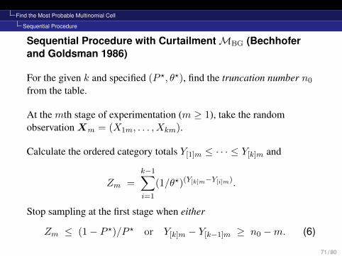
Sequential Procedure with CurtailmentMBG (Bechhoferand Goldsman 1986)
For the given k and specified (P ?, θ?), find the truncation number n0
from the table.
At the mth stage of experimentation (m ≥ 1), take the randomobservationXm = (X1m, . . . , Xkm).
Calculate the ordered category totals Y[1]m ≤ · · · ≤ Y[k]m and
Zm =k−1∑i=1
(1/θ?)(Y[k]m−Y[i]m).
Stop sampling at the first stage when either
Zm ≤ (1− P ?)/P ? or Y[k]m − Y[k−1]m ≥ n0 −m. (6)
71 / 80

Find the Most Probable Multinomial Cell
Sequential Procedure
Let N denote the value of m at the termination of sampling. Selectthe category that yielded Y[k]N as the one associated with p[k];randomize in the case of ties.
Remark: The truncation numbers n0 given in the previous table arecalculated assuming that ProcedureMBG has the sameLF-configuration (3) as doesMBEM. (This hasn’t been proven yet.)
Example: Suppose k = 3, P ? = 0.75, and θ? = 3.0. The table tells usto truncate sampling at n0 = 5 observations. For the data
m X1m X2m X3m Y1m Y2m Y3m
1 0 1 0 0 1 0
2 0 1 0 0 2 0
we stop sampling by the first criterion in (6) becauseZ2 = (1/3)2 + (1/3)2 = 2/9 ≤ (1− P ?)/P ? = 1/3, and we selectcategory 2. 2
72 / 80

Find the Most Probable Multinomial Cell
Sequential Procedure
Example: Again suppose k = 3, P ? = 0.75, and θ? = 3.0 (so thatn0 = 5). For the data
m X1m X2m X3m Y1m Y2m Y3m
1 0 1 0 0 1 0
2 1 0 0 1 1 0
3 0 1 0 1 2 0
4 1 0 0 2 2 0
5 1 0 0 3 2 0
we stop sampling by the second criterion in (6) because m = n0 = 5observations, and we select category 1. 2
73 / 80

Find the Most Probable Multinomial Cell
Sequential Procedure
Example: Yet again suppose k = 3, P ? = 0.75, and θ? = 3.0 (so thatn0 = 5). For the data
m X1m X2m X3m Y1m Y2m Y3m
1 0 1 0 0 1 0
2 1 0 0 1 1 0
3 0 1 0 1 2 0
4 1 0 0 2 2 0
5 0 0 1 2 2 1
we stop according to the second criterion in (6) because m = n0 = 5.However, we now have a tie between Y1,5 and Y2,5 and thus randomlyselect between categories 1 and 2. 2
74 / 80

Find the Most Probable Multinomial Cell
Sequential Procedure
Example: Still yet again suppose k = 3, P ? = 0.75, and θ? = 3.0 (sothat n0 = 5). Suppose we observe
m X1m X2m X3m Y1m Y2m Y3m
1 0 1 0 0 1 0
2 1 0 0 1 1 0
3 0 1 0 1 2 0
4 0 0 1 1 2 1
Because categories 1 and 3 can do no better than tie category 2 (if wewere to take the potential remaining n0 −m = 5− 4 = 1observation), the second criterion in (6) tells us to stop; we selectcategory 2. 2
75 / 80
Find the Most Probable Multinomial Cell
Sequential Procedure
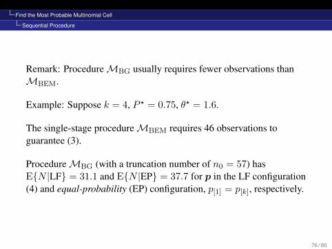
Remark: ProcedureMBG usually requires fewer observations thanMBEM.
Example: Suppose k = 4, P ? = 0.75, θ? = 1.6.
The single-stage procedureMBEM requires 46 observations toguarantee (3).
ProcedureMBG (with a truncation number of n0 = 57) hasE{N |LF} = 31.1 and E{N |EP} = 37.7 for p in the LF configuration(4) and equal-probability (EP) configuration, p[1] = p[k], respectively.
76 / 80

Find the Most Probable Multinomial Cell
Nonparametric Applications
Nonparametric ApplicationsLet’s take i.i.d. vector-observationsWj = (W1j , . . . ,Wkj) (j ≥ 1),where the Wij can be either discrete or continuous.
For a particular vector-observationWj , suppose the experimenter candetermine which of the k observations Wij (1 ≤ i ≤ k) is the “mostdesirable.” The term “most desirable” is based on some criterion ofgoodness designated by the experimenter, and it can be quite general,e.g.,. . .
The largest crop yield based on a vector-observation of kagricultural plots using competing fertilizers.
The smallest sample average customer waiting time based on asimulation run of each of k competing queueing strategies.
The smallest estimated variance of customer waiting times (fromthe above simulations).
77 / 80

Find the Most Probable Multinomial Cell
Nonparametric Applications
For a particular vector-observationWj , suppose Xij = 1 or 0according as Wij (1 ≤ i ≤ k) is the “most desirable” of thecomponents ofWj or not. Then (X1j , . . . , Xkj) (j ≥ 1) has amultinomial distribution with probability vector p, where
pi = P{Wi1 is the “most desirable” component ofW1}.
Selection of the category corresponding to the largest pi can bethought of as that of finding the component having the highestprobability of yielding the “most desirable” observation of those froma particular vector-observation. This problem can be approachedusing the multinomial selection methods described in this module.
78 / 80
Find the Most Probable Multinomial Cell
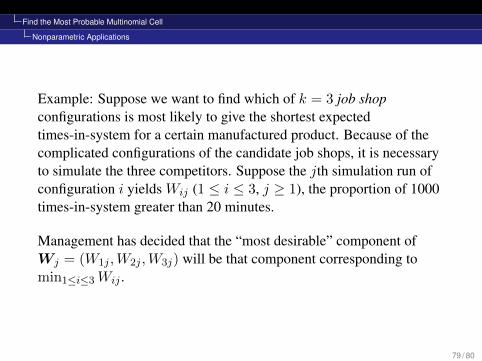
Nonparametric Applications
Example: Suppose we want to find which of k = 3 job shopconfigurations is most likely to give the shortest expectedtimes-in-system for a certain manufactured product. Because of thecomplicated configurations of the candidate job shops, it is necessaryto simulate the three competitors. Suppose the jth simulation run ofconfiguration i yields Wij (1 ≤ i ≤ 3, j ≥ 1), the proportion of 1000times-in-system greater than 20 minutes.
Management has decided that the “most desirable” component ofWj = (W1j ,W2j ,W3j) will be that component corresponding tomin1≤i≤3Wij .
79 / 80
Find the Most Probable Multinomial Cell
Nonparametric Applications
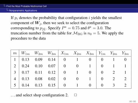
If pi denotes the probability that configuration i yields the smallestcomponent ofWj , then we seek to select the configurationcorresponding to p[3]. Specify P ? = 0.75 and θ? = 3.0. Thetruncation number from the table forMBG is n0 = 5. We apply theprocedure to the data
m W1m W2m W3m X1m X2m X3m Y1m Y2m Y3m
1 0.13 0.09 0.14 0 1 0 0 1 0
2 0.24 0.10 0.07 0 0 1 0 1 1
3 0.17 0.11 0.12 0 1 0 0 2 1
4 0.13 0.08 0.02 0 0 1 0 2 2
5 0.14 0.13 0.15 0 1 0 0 3 2
. . . and select shop configuration 2. 2
80 / 80


