
Gasoline consumptionefficiency:An equivalence estimate from energydemand function and production function
David C. BroadstockXiaoqi ChenJune 2017, Singapore

BACKGROUND
I There are two fundamental approaches to obtaining measures ofenergy efficiency. One can choose to take either the traditionalapproach embedded in the context of classical production theory, orinstead follow more recently devised methods grounded in demandtheory (Filippini and Hunt 2011).
I Given the absence of academic literature for the comparison ofproduction function and consumer function, we analyze thetheories and discuss the connections between these two different wayson measure gasoline consumption efficiency.
MOTIVATIONS
I In 2015, President Xi in China put forwarded "Supply Side StructuralReform" and "Demand Expansion". As policy maker, they want toknow what is the most efficiency way to implement the reform policy:demand side or production side.
I If our results hold, it would suggest that in certain cases we can useefficiency estimates from a demand function as a proxy for productionrelated efficiency and vice versa.
I Energy demand function is derived form production function. We canregard energy as a final product and service.

PRESENTATION OUTLINEA presentation in two or three parts, depending on your preferences
I Specify and estimate a ‘Frontier demand function’I Specify and estimate an ‘inverted production function’ (energy
oriented sub-vector input distance function)
I Compare estimates of gasoline efficiency obtained using these twoapproaches
I This stage of comparison is somehow optional to the reader - it is a simpleinterpretive exercise, and the estimates of a gasoline demand function anda general production function hold value even without these comparisons
I We note that:I The demand function provides a consumer theory motivated measure of
efficiencyI Conversely the production function adopts a producer-theory based view
of efficiency
DATA CONSIDERATIONS
There are a number of data sources that can be consulted, although a singleconsistent source is not a luxury that should be taken for granted.
I Main variable is gasoline consumption per capitaI Data cover the years 1995-2014I We exclude TibetI China Energy Statistical YearbookI National Bureau of Statistics of People’s Republic of ChinaI Bloomberg database (HDD, CDD)

SOME KEY STATISTICS AND TRENDSAn initial glance at the trend of gasoline
●● ●
●
● ●●
●●
●
●
●
●
●
●
●
●
●
●
●
1995 1998 2001 2004 2007 2010 2013
020
040
060
080
010
0012
00
Consumption of Gasoline
BeijingShanghai
●●
●
●
●
●
●
●
●
●
●
●
● ●
●
●
●
●
●
●
●●
●●
●
●
●
●
●
●
● ●●
●
●
●
●
●
●
1995 1998 2001 2004 2007 2010 2013
0.00
0.05
0.10
0.15
0.20
Consumption of Gasoline per capital
(10
000
tons
)
BeijingShanghai

ECONOMETRIC DEMAND FUNCTION SET-UPSFA model
git = a + appit + ay yit + ahdd hddit + acdd cddit + at t + at2t2 + vit + uit
For the frontier demand function approach, the present study mimics closely theempirical specification of Filippini and Zhang (2011).
I Price (based on 1995)I Income (natural logarithm of of GDP)I weather proxiesI UEDT ( Underlying Energy Demand Trends)I vit (the normal noise term assumed to be normally distributed.)I uit (contains information on the distance between the frontier and the actual input
and is interpreted as an indicator of the inefficiency levels.

DEMAND FUNCTION ESTIMATION RESULTS
I Income elasticitiy a-prioriI Price elasticitiy a-prioriI Dummies for coastal and
city (Coastal:Tianjin LiaoningHebei Shandong JiangsuZhejiang Shanghai FujianGuangdong GuangxiHainanCity: Beijing ChongqingShanghai Tianjin )
Estimation method: ——————— SFA ———————Model specification: (1) (2) (3) (4)
Estimated coefficientsIntercept -1.531 -1.385 -2.021∗ -1.873∗
Income (Y) 1.078∗∗∗ 1.019∗∗∗ 0.979∗∗∗ 0.925 ∗∗∗
Price of gasoline (P) -0.653∗∗∗ -0.702∗∗∗ -0.616∗∗∗ -0.649 ∗∗∗
Heating degree days (HDD) 0.026 0.033 0.041 0.046
Cooling degree days (CDD) 0.111 0.102 0.118∗ 0.103
Time 0.028∗ 0.037∗ 0.033 ∗ 0.039∗∗
Time squared -0.002∗∗∗ -0.002∗∗∗ -0.001 ∗∗∗ -0.002∗∗∗
Coastal dummy 0.160 ∗ 0.172∗
City-province dummy 0.209 ∗ 0.224∗
Model diagnostics/additional informationObservations 600 600 600 600Provinces 30 30 30 30Years 20 20 20 20log-likelihood values -10.860 -8.861 -8.936 -6.699
Note: ∗∗ These tests are comparing only models using the same estimation method.
THE INVERTED PRODUCTION FUNCTIONSFA model
-git = β0+βl lit +βk kit +βy yit +βkekeit +βngngit +βccit +βl,l l2it +βk,k k2
it +βy,y y2it +
βke,keke2it +βng,ngng2
it +βc,cc2it +βl,k [lit ∗kit ]+βl,y [lit ∗yit ]+...+at t+at2
t2+Vit +Uit
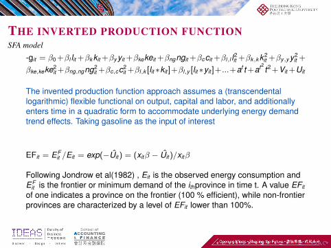
The invented production function approach assumes a (transcendentallogarithmic) flexible functional on output, capital and labor, and additionallyenters time in a quadratic form to accommodate underlying energy demandtrend effects. Taking gasoline as the input of interest
EFit = EFit /Eit = exp(−Uit) = (xitβ − Uit)/xitβ
Following Jondrow et al(1982) , Eit is the observed energy consumption andEF
it is the frontier or minimum demand of the ithprovince in time t. A value EFit
of one indicates a province on the frontier (100 % efficient), while non-frontierprovinces are characterized by a level of EFit lower than 100%.

THE INVERTED PRODUCTION FUNCTIONIt is difficult to ‘validate’ these estimates directly
Variables ——————— SFA ———————(1) (2) (3) (4)
Estimated coefficients(level terms)βy -1.843 ∗∗∗ -1.859 ∗∗∗ -1.807 ∗∗∗ -1.826 ***βc 0.526∗ 0.513∗ 0.540∗ 0.529∗
(squared-terms)βy2 -0.120 ∗∗ -0.115 ∗∗ -0.116 ∗∗ -0.114 ∗∗
βng2 0.003 ∗ 0.003∗ 0.004∗ 0.004∗
(cross-products)βy,c 0.228 ∗∗∗ 0.227 ∗∗∗ 0.224 ∗∗∗ 0.225∗∗∗
βy,k 0.212 ∗∗∗ 0.204 ∗∗∗ 0.215 ∗∗∗ 0.208∗∗∗
βy,cok -0.086 ∗∗ -0.086 ∗∗∗ -0.086 ∗∗∗ -0.086∗∗∗
βc,k -0.191 ∗∗ -0.182 ∗∗ -0.194 ∗∗ -0.187 ∗∗
βk,cok 0.077 ∗ 0.076 ∗ 0.079∗ 0.078 ∗
(other variables)βt2 0.001 ∗∗∗ 0.001 ∗∗∗ 0.001 ∗∗∗
βcoastal -0.088 -0.069βcity 0.129 0.108

DO THE TWO SHOW SOME SIMILARITIESOn the strength of the statistical correlations between the efficiencies
The pattern of correlation between the scores is not, perfect, but is very high with a net
correlation across all years well in excess of 0.9. This implies a high degree of
observational equivalence between the scores from the two alternative approaches.
●
●
●
●
●
●
●
●
●
●
●
●
●
●
●
●●
● ●
●
●●
●●
●●
●
●●
●
0.0 0.2 0.4 0.6 0.8 1.0
0.0
0.2
0.4
0.6
0.8
1.0
Year 2000
Demand efficiency
Pro
duct
ion
effic
ienc
y
●
●
●
●
●
●
●
●
●
●
●
●
●
●
●
●●
● ●
●
●●
●●
●●
●
●●
●
0.0 0.2 0.4 0.6 0.8 1.0
0.0
0.2
0.4
0.6
0.8
1.0
Year 2014
Demand efficiency
Pro
duct
ion
effic
ienc
y
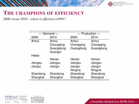
THE CHAMPIONS OF EFFICIENCY2000 versus 2014 - where is efficiency>90%?
— Demand — — Production —2000 2014 2000 2014Anhui Anhui Anhui Anhui
Chongqing Chongqing ChongqingGuangdong Guangdong GuangdongGuangxi
HebeiHenan Henan Henan
Jiangsu Jiangsu Jiangsu JiangsuJiangxi Jiangxi Jiangxi Jiangxi
Ningxia NingxiaShandong Shandong Shandong ShandongShanghai Shanghai Shanghai Shanghai

CONCLUSIONSWhat can we learn from this study so far?
I This paper compares and contrasts the efficiency scores obtained fromtwo popular re- cent model variants. A surprising degree ofobservational equivalence is found, at least in the context of Chinesegasoline consumption efficiency. In light of this the study will seek toelaborate on the reasons which might imply equivalence and whatimplica- tions/opportunities this might create energy policy.

THANKS FOR [email protected]


