
Gaussian processes for uncertainty quantification incomputer experiments
Richard Wilkinson
University of Nottingham
Gaussian process summer school, Sheffield 2013
Richard Wilkinson (Nottingham) GPs for UQ in DACE June 2013 1 / 70

Talk plan
(a) UQ and computer experiments
(b) Gaussian process emulators
(c) 3 examples:
(i) calibration using emulators(ii) simulator discrepancy modelling(iii) accelerating ABC using GPs
Richard Wilkinson (Nottingham) GPs for UQ in DACE June 2013 2 / 70

Computer experiments
Baker 1977 (Science):
‘Computerese is the new lingua franca of science’
Rohrlich (1991): Computer simulation is
‘a key milestone somewhat comparable to the milestone thatstarted the empirical approach (Galileo) and the deterministicmathematical approach to dynamics (Newton and Laplace)’
The gold-standard of empirical research is the designed experiment, whichusually involves concepts such as replication, blocking, and randomization.
However, in the past three decades computer experiments (in silicoexperiments) have become commonplace in nearly all fields.
Richard Wilkinson (Nottingham) GPs for UQ in DACE June 2013 3 / 70

EngineeringCarbon capture and storage technology - PANACEA project
Knowledge about the geology of the wells is uncertain.
Richard Wilkinson (Nottingham) GPs for UQ in DACE June 2013 4 / 70

Climate SciencePredicting future climate
Richard Wilkinson (Nottingham) GPs for UQ in DACE June 2013 5 / 70

Challenges of computer experimentsClimate Predictions
Richard Wilkinson (Nottingham) GPs for UQ in DACE June 2013 6 / 70

Challenges for statistics
The statistical challenges posed by computer experiments are somewhatdifferent to physical experiments and have only recently begun to betackled by statisticians.
For example, replication, randomization and blocking are irrelevantbecause a computer model will give identical answers if run multiple times.
Key questions: How do we make inferences about the world from asimulation of it?
how do we relate simulators to reality? (model error)
how do we estimate tunable parameters? (calibration)
how do we deal with computational constraints? (stat. comp.)
how do we make uncertainty statements about the world thatcombine models, data and their corresponding errors? (UQ)
There is an inherent a lack of quantitative information on the uncertaintysurrounding a simulation - unlike in physical experiments.
Richard Wilkinson (Nottingham) GPs for UQ in DACE June 2013 7 / 70
Incorporating and accounting for uncertainty
Perhaps the biggest challenge faced is incorporating uncertainty incomputer experiments.
We are used to dealing with uncertainty in physical experiments. But ifyour computer model is deterministic, there is no natural source ofvariation and so the experimenter must carefully assess where errors mightarise.
Types of uncertainty:
Parametric uncertainty
Model inadequacy
Observation errors
Code uncertainty
Richard Wilkinson (Nottingham) GPs for UQ in DACE June 2013 8 / 70
Code uncertaintyWe think of the simulator as a function
η : X → YTypically both the input and output space will be subsets of Rn for somen.
Monte Carlo (brute force) methods can be used for most tasks if sufficientcomputational resource is available.
For example, uncertainty analysis is finding the distribution of η(θ) whenθ ∼ π(·):
draw a sample of parameter values from the prior θ1, . . . , θN ∼ π(θ),
Look at η(θ1), . . . , η(θN) to find the distribution π(η(θ)).
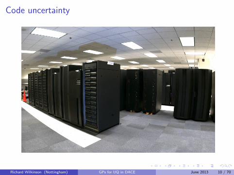
However, for complex simulators, run times might be long.Consequently, we will only know the simulator output at a finite numberof points:
code uncertainty
Richard Wilkinson (Nottingham) GPs for UQ in DACE June 2013 9 / 70

Code uncertaintyWe think of the simulator as a function
η : X → YTypically both the input and output space will be subsets of Rn for somen.
Monte Carlo (brute force) methods can be used for most tasks if sufficientcomputational resource is available.For example, uncertainty analysis is finding the distribution of η(θ) whenθ ∼ π(·):
draw a sample of parameter values from the prior θ1, . . . , θN ∼ π(θ),
Look at η(θ1), . . . , η(θN) to find the distribution π(η(θ)).
However, for complex simulators, run times might be long.Consequently, we will only know the simulator output at a finite numberof points:
code uncertaintyRichard Wilkinson (Nottingham) GPs for UQ in DACE June 2013 9 / 70
Code uncertainty
Richard Wilkinson (Nottingham) GPs for UQ in DACE June 2013 10 / 70

Code uncertainty
For slow simulators, we are uncertain about the simulator value at allpoints except those in a finite set.
All inference must be done using a finite ensemble of model runs
Dsim = {(θi , η(θi ))}i=1,...,N
If θ is not in the ensemble, then we are uncertainty about the valueof η(θ).
If θ is multidimensional, then even short run times can rule out bruteforce approaches
θ ∈ R10 then 1000 simulator runs is only enough for one point ineach corner of the design space.
Richard Wilkinson (Nottingham) GPs for UQ in DACE June 2013 11 / 70

Meta-modelling
Idea: If the simulator is expensive, build a cheap model of it and use thisin any analysis.
‘a model of the model’
We call this meta-model an emulator of our simulator.
We use the emulator as a cheap approximation to the simulator.
ideally an emulator should come with an assessment of its accuracy
rather just predict η(θ) it should predict π(η(θ)|Dsim) - ouruncertainty about the simulator value given the ensemble Dsim.
Richard Wilkinson (Nottingham) GPs for UQ in DACE June 2013 12 / 70

Meta-modellingGaussian Process Emulators
Gaussian processes provide a flexible nonparametric distributions for ourprior beliefs about the functional form of the simulator:
η(·) ∼ GP(m(·), σ2c(·, ·))
where m(·) is the prior mean function, and c(·, ·) is the prior covariancefunction (semi-definite).
If we observe the ensemble of model runs Dsim, then update our priorbelief about η in light of the ensemble of model runs:
η(·)|Dsim ∼ GP(m∗(·), σ2c∗(·, ·))
where m∗ and c∗ are the posterior mean and covariance functions (simplefunctions of Dsim, m and c).
Richard Wilkinson (Nottingham) GPs for UQ in DACE June 2013 13 / 70

Gaussian Process IllustrationZero mean
0 2 4 6 8 10
−2
02
46
810
Prior Beliefs
X
Y
Richard Wilkinson (Nottingham) GPs for UQ in DACE June 2013 14 / 70

Gaussian Process Illustration
0 2 4 6 8 10
−2
02
46
810
Ensemble of model evaluations
X
Y
Richard Wilkinson (Nottingham) GPs for UQ in DACE June 2013 15 / 70

Gaussian Process Illustration
0 2 4 6 8 10
−2
02
46
810
Posterior beliefs
X
Y
Richard Wilkinson (Nottingham) GPs for UQ in DACE June 2013 16 / 70
Emulator choices
η(x) = h(x)β + u(x)
emulator = mean structure + residual
u(x) can be taken to be a zero-mean Gaussian process
u(·) ∼ GP(0, c(·, ·))
Emulator choices:
mean structure h(x)I 1, x , x2, . . ., Legendre polynomials?I Allows us to build in known trends and exploit power of linear
regression
covariance function c(·, ·) - cf Nicolas’ talkI Stationary? Smooth?I Length-scale?I Nb - we don’t a nugget term
Richard Wilkinson (Nottingham) GPs for UQ in DACE June 2013 17 / 70

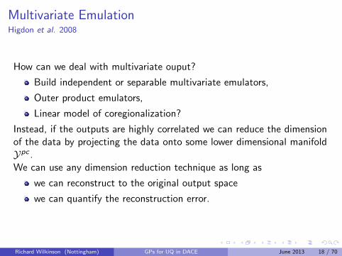
Multivariate EmulationHigdon et al. 2008
How can we deal with multivariate ouput?
Build independent or separable multivariate emulators,
Outer product emulators,
Linear model of coregionalization?
Instead, if the outputs are highly correlated we can reduce the dimensionof the data by projecting the data onto some lower dimensional manifoldYpc .We can use any dimension reduction technique as long as
we can reconstruct to the original output space
we can quantify the reconstruction error.
Richard Wilkinson (Nottingham) GPs for UQ in DACE June 2013 18 / 70

Multivariate EmulationHigdon et al. 2008
How can we deal with multivariate ouput?
Build independent or separable multivariate emulators,
Outer product emulators,
Linear model of coregionalization?
Instead, if the outputs are highly correlated we can reduce the dimensionof the data by projecting the data onto some lower dimensional manifoldYpc .
We can use any dimension reduction technique as long as
we can reconstruct to the original output space
we can quantify the reconstruction error.
Richard Wilkinson (Nottingham) GPs for UQ in DACE June 2013 18 / 70
Multivariate EmulationHigdon et al. 2008
How can we deal with multivariate ouput?
Build independent or separable multivariate emulators,
Outer product emulators,
Linear model of coregionalization?
Instead, if the outputs are highly correlated we can reduce the dimensionof the data by projecting the data onto some lower dimensional manifoldYpc .We can use any dimension reduction technique as long as
we can reconstruct to the original output space
we can quantify the reconstruction error.
Richard Wilkinson (Nottingham) GPs for UQ in DACE June 2013 18 / 70

We can then emulate the function that maps the input space Θ to thereduced dimensional output space Ypc , i.e., ηpc(·) : Θ→ Ypc
It doesn’t matter what dimension reduction scheme we use, as long as wecan reconstruct from Ypc and quantify the error in the reconstruction.
Richard Wilkinson (Nottingham) GPs for UQ in DACE June 2013 19 / 70
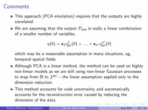
Comments
This approach (PCA emulation) requires that the outputs are highlycorrelated.
We are assuming that the output Dsim is really a linear combinationof a smaller number of variables,
η(θ) = v1η1pc(θ) + . . .+ vn∗ηn∗
pc (θ)
which may be a reasonable assumption in many situations, eg,temporal spatial fields.
Although PCA is a linear method, the method can be used on highlynon-linear models as we are still using non-linear Gaussian processesto map from Θ to Ypc – the linear assumption applied only to thedimension reduction.
This method accounts for code uncertainty and automaticallyaccounts for the reconstruction error caused by reducing thedimension of the data.
Richard Wilkinson (Nottingham) GPs for UQ in DACE June 2013 20 / 70

Example 1: Calibration
Richard Wilkinson (Nottingham) GPs for UQ in DACE June 2013 21 / 70

CalibrationInverse problems
For forwards models we specify parameters θ and i.c.s and the modelgenerates output Dsim. Usually, we are interested in the inverse-problem,i.e., observe data Dfield , want to estimate parameter values.
We have three sources of information that we wish to combine
1 Scientific knowledge captured by the model, η
2 Empirical information contained in the data, Dfield
3 Expert opinion based upon experience.
We want to combine all three sources to produce the ‘best’ parameterestimates we can.
Richard Wilkinson (Nottingham) GPs for UQ in DACE June 2013 22 / 70

Carbon feedbacks
Terrestrial ecosystems currently absorb a considerable fraction ofanthropogenic carbon emissions.
However, the fate of this sink is highly uncertain due to insufficientknowledge about key feedbacks.
I We are uncertain about the sensitivity of soil respiration to increasingglobal temperature.
I GCM predictions don’t agree on the sign of the net terrestrial carbonflux.
The figure shows inter-model spread in uncalibrated GCM modelpredictions.
How much additional spread is there from parametric uncertainty?(as opposed to model structural uncertainty?)
Would calibration reduce the range of the ensemble predictions? Orwould it increase our uncertainty?
We can’t answer these questions with full GCMs at present, but we canbegin to investigate with simplified EMIC models.
Richard Wilkinson (Nottingham) GPs for UQ in DACE June 2013 23 / 70

Carbon feedbacks
Terrestrial ecosystems currently absorb a considerable fraction ofanthropogenic carbon emissions.
However, the fate of this sink is highly uncertain due to insufficientknowledge about key feedbacks.
I We are uncertain about the sensitivity of soil respiration to increasingglobal temperature.
I GCM predictions don’t agree on the sign of the net terrestrial carbonflux.
The figure shows inter-model spread in uncalibrated GCM modelpredictions.
How much additional spread is there from parametric uncertainty?(as opposed to model structural uncertainty?)
Would calibration reduce the range of the ensemble predictions? Orwould it increase our uncertainty?
We can’t answer these questions with full GCMs at present, but we canbegin to investigate with simplified EMIC models.Richard Wilkinson (Nottingham) GPs for UQ in DACE June 2013 23 / 70

Friedlingstein et al. 2006 - ‘uncalibrated’ GCM carbon cycle predictions
Climate simulators tend to be ‘tuned’ rather than calibrated, due to their complexity.
Richard Wilkinson (Nottingham) GPs for UQ in DACE June 2013 24 / 70

UVic Earth System Climate ModelRicciutio et al. 2011, Wilkinson 2010
UVic ESCM is an intermediate complexity model with a generalcirculation ocean and dynamic/thermodynamic sea-ice componentscoupled to a simple energy/moisture balance atmosphere. It has adynamic vegetation and terrestrial carbon cycle model (TRIFFID) as wellas an inorganic carbon cycle.
Inputs: Q10 = soil respiration sensitivity to temperature (carbonsource) and Kc = CO2 fertilization of photosynthesis (carbon sink).
Output: time-series of CO2 values, cumulative carbon fluxmeasurements, spatial-temporal field of soil carbon measurements.
The observational data are limited, and consist of 60 measurementsDfield :
40 instrumental CO2 measurements from 1960-1999 (the Mauna Loadata)
17 ice core CO2 measurements
3 cumulative ocean carbon flux measurements
Richard Wilkinson (Nottingham) GPs for UQ in DACE June 2013 25 / 70

UVic Earth System Climate ModelRicciutio et al. 2011, Wilkinson 2010
UVic ESCM is an intermediate complexity model with a generalcirculation ocean and dynamic/thermodynamic sea-ice componentscoupled to a simple energy/moisture balance atmosphere. It has adynamic vegetation and terrestrial carbon cycle model (TRIFFID) as wellas an inorganic carbon cycle.
Inputs: Q10 = soil respiration sensitivity to temperature (carbonsource) and Kc = CO2 fertilization of photosynthesis (carbon sink).
Output: time-series of CO2 values, cumulative carbon fluxmeasurements, spatial-temporal field of soil carbon measurements.
The observational data are limited, and consist of 60 measurementsDfield :
40 instrumental CO2 measurements from 1960-1999 (the Mauna Loadata)
17 ice core CO2 measurements
3 cumulative ocean carbon flux measurementsRichard Wilkinson (Nottingham) GPs for UQ in DACE June 2013 25 / 70

CalibrationThe aim is to combine the physics coded into UVic with the empiricalobservations to learn about the carbon feedbacks.However, UVic takes approximately two weeks to run for a single inputconfiguration. Consequently, all inference must be done from a limitedensemble of model runs.
48 member ensemble, grid design D, output Dsim (48× n).
1.0 1.5 2.0 2.5 3.0 3.5 4.0
0.5
1.0
1.5
Q10
Kc
- this is overkill for this model - benefit of sequential designsRichard Wilkinson (Nottingham) GPs for UQ in DACE June 2013 26 / 70

Model runs and data
1800 1850 1900 1950 2000
280
300
320
340
360
380
400
year
CO
2 level
Richard Wilkinson (Nottingham) GPs for UQ in DACE June 2013 27 / 70

PC Plots
1800 1850 1900 1950 2000
0.0
00
.05
0.1
00
.15
0.2
0
Leading Principal Component
year
PC
1
1800 1850 1900 1950 2000
−0
.10
−0
.05
0.0
00
.05
0.1
00
.15
Second Principal Component
year
PC
2
Leading PC Loading with Data Projection
Q10
Kc
1.0 1.5 2.0 2.5 3.0 3.5 4.0
0.5
1.0
1.5
Second PC Loading with Data Projection
Q10
Kc
1.0 1.5 2.0 2.5 3.0 3.5 4.0
0.5
1.0
1.5
Richard Wilkinson (Nottingham) GPs for UQ in DACE June 2013 28 / 70

Diagnostics
Diagnostic checks are vital if we are to trust the use of the emulator inplace of the simulator.
For the PC emulator, we ultimately want to predict the spatial field - somost diagnostic effort should be spent on the reconstructed emulator.
Looking only at the percentage of variance explained by the principalcomponents can be misleading, even if the emulators are perfect, as wecan find that PCs that have small eigenvalues (so explain a small amountof variance) can play an important role in prediction.
Richard Wilkinson (Nottingham) GPs for UQ in DACE June 2013 29 / 70

Leave-one-out (LOA) plots for PC1Leave-one-out plots are a type of cross-validation to asses whether thefinal emulator is working well both in terms of the mean prediction, andthe uncertainty estimates.
We leave each ensemble member, we leave it out of the training set andbuild a new emulator. We then predict the left-out ensemble memberusing the emulator
−50
50
150
250
OSA plot for PC score 1
Run Number
Score
1 2 3 4 5 39 6 7 8 9 10 11 12 13 14 15 16 17 18 40 41 42 43 44 19 20 21 22 23 24 45 46 25 26 27 28 47 48 29 30 31 32 33 34 35 36 37 38
−50
50
150
250
LOO for PC score 1
Run Number
Score
1 2 3 4 5 39 6 7 8 9 10 11 12 13 14 15 16 17 18 40 41 42 43 44 19 20 21 22 23 24 45 46 25 26 27 28 47 48 29 30 31 32 33 34 35 36 37 38
We would like accurate coverage.Richard Wilkinson (Nottingham) GPs for UQ in DACE June 2013 30 / 70

One-step-ahead (OSA) plots for PC1
One-step-ahead diagnostics are created by first ordering the ensembleaccording to one of the input variables, in this case θ1. We then train anemulator using only the first n − 1 ensemble members, before predictingthe nth ensemble member.
One-step-ahead diagnostics primarily test whether the uncertaintyestimates of the emulator are accurate. Because the size of the ensemblegrows, we can check more easily whether the length-scale and covariancestructure of the emulator are satisfactory.
−50
50
150
250
OSA plot for PC score 1
Run Number
Score
1 2 3 4 5 39 6 7 8 9 10 11 12 13 14 15 16 17 18 40 41 42 43 44 19 20 21 22 23 24 45 46 25 26 27 28 47 48 29 30 31 32 33 34 35 36 37 38
−50
50
150
250
LOO for PC score 1
Run Number
Score
1 2 3 4 5 39 6 7 8 9 10 11 12 13 14 15 16 17 18 40 41 42 43 44 19 20 21 22 23 24 45 46 25 26 27 28 47 48 29 30 31 32 33 34 35 36 37 38
Richard Wilkinson (Nottingham) GPs for UQ in DACE June 2013 31 / 70

Calibration FrameworkKennedy and O’Hagan 2001
Assume that reality ζ(t) is the computer model run at the ‘true’ value ofthe parameter θ̂ plus model error:
ζ(t) = η(t, θ̂) + δ(t)
We observe reality plus noise:
Dfield (t) = ζ(t) + ε(t)
so thatDfield (t) = η(t, θ̂) + δ(t) + ε(t).
We then aim to find π(θ̂|Dsim,Dfield ).
Richard Wilkinson (Nottingham) GPs for UQ in DACE June 2013 32 / 70

Model DiscrepancyThe calibration framework used is:
Dfield (t) = η(θ, t) + δ(t) + ε(t)
The model predicts the underlying trend, but real climate fluctuatesaround this. We model
discrepancy as an AR1 process: δ(0) ∼ N(0, σ2δ ), and
δ(t) = ρδ(t − 1) + N(0, σ2δ ).
Measurement error as heteroscedastic independent random noiseε(t) ∼ N(0, λ(t)).
5 10 15
−0.2
0.0
0.2
0.4
0.6
0.8
Lag
Part
ial A
CF
Once we have specified all these choices, we can then find the posteriorusing an MCMC scheme.Richard Wilkinson (Nottingham) GPs for UQ in DACE June 2013 33 / 70

Results
Q10
0.5 1.0 1.5
0.80 0.0066
−80 −60 −40 −20 0 20 40
1.0
2.0
3.0
4.0
0.0095
0.5
1.0
1.5 Kc
0.009 0.009
sigma2
10
00
20
00
30
00
40
00
0.011
1.0 1.5 2.0 2.5 3.0 3.5 4.0
−8
0−
40
04
0
1000 1500 2000 2500 3000 3500 4000
beta
Richard Wilkinson (Nottingham) GPs for UQ in DACE June 2013 34 / 70

Example 2: simulator discrepancy
Richard Wilkinson (Nottingham) GPs for UQ in DACE June 2013 35 / 70

All models are wrong, but ...Kennedy and O’Hagan 2001
Lets acknowledge that most models are imperfect.
Consequently,
predictions will be wrong, or will be made with misleading degree ofconfidence
solving the inverse problem y(x) = f (x , θ) + e may not give sensibleestimates of θ.
I e is measurement errorI f (x , θ) is our computer modelI y is our data
Can we
account for the error?
correct the error?
Richard Wilkinson (Nottingham) GPs for UQ in DACE June 2013 36 / 70

All models are wrong, but ...Kennedy and O’Hagan 2001
Lets acknowledge that most models are imperfect. Consequently,
predictions will be wrong, or will be made with misleading degree ofconfidence
solving the inverse problem y(x) = f (x , θ) + e may not give sensibleestimates of θ.
I e is measurement errorI f (x , θ) is our computer modelI y is our data
Can we
account for the error?
correct the error?
Richard Wilkinson (Nottingham) GPs for UQ in DACE June 2013 36 / 70

Dynamic modelsWilkinson et al. 2011
Kennedy and O’Hagan (2001) suggested we introduce reality ζ into ourstatistical inference
Reality ζ(x) = f (x , θ̂) + δ(x), the best model prediction plus modelerror δ(x).
Data y(x) = ζ(x) + e where e represents measurement error
In many cases, we may have just a single realisation from which to learn δ
For dynamical systems the model sequentially makes predictions beforethen observing the outcome.
Embedded in this process is information about how well the modelperforms for a single time-step.
We can specify a class of models for the error, and then try to learnabout the error from our predictions and the realised data.
Richard Wilkinson (Nottingham) GPs for UQ in DACE June 2013 37 / 70

Mathematical Framework
Suppose we have
State vector xt which evolves through time. Let x0:T denote(x0, x1, . . . , xT ).
Computer model f which encapsulates our beliefs about thedynamics of the state vector
xt+1 = f (xt , ut)
which depends on forcings ut . We treat f as a black-box.
Observationsyt = h(xt)
where h(·) usually contains some stochastic element
Richard Wilkinson (Nottingham) GPs for UQ in DACE June 2013 38 / 70

Moving from white to coloured noise
A common approach is to treat the model error as white noise
State evolution: xt+1 = f (xt , ut) + εt where εt are iid rvs.
Instead of the white noise model error, we ask whether there is a strongersignal that could be learnt:
State evolution: xt+1 = f (xt , ut) + δ(xt , ut) + εt
Observations: yt = h(xt).
Our aim is to learn a functional form plus stochastic error description of δ
Richard Wilkinson (Nottingham) GPs for UQ in DACE June 2013 39 / 70

Why this is difficult?
x0:T is usually unobserved, but given observations y0:T and a fullyspecified model we can infer x0:T .
I the filtering/smoothing problem
When we want to learn the discrepancy δ(x) we are in the situationwhere we estimate δ from x0:T , . . .
but we must estimate x0:T from a description of δ.
Richard Wilkinson (Nottingham) GPs for UQ in DACE June 2013 40 / 70

Toy Example: Freefall
Consider an experiment where we drop a weightfrom a tower and measure its position xt every∆t seconds.
Noisy observation: yn ∼ N(xn, σ2obs)
Suppose we are given a computer model based on
dv
dt= g
Which gives predictions at the observations of
xn+1 = xn + vk ∆t + 12g(∆t)2
vn+1 = vn + g∆t
Richard Wilkinson (Nottingham) GPs for UQ in DACE June 2013 41 / 70

Toy Example: Freefall
Assume that the ‘true’ dynamics include aStokes’ drag term
dv
dt= g − kv
Which gives single time step updates
xn+1 = xn +1
k(g
k− vt)(e−k∆t − 1) +
g∆t
k
vn+1 = (vn −g
k)e−k∆t +
g
k
Richard Wilkinson (Nottingham) GPs for UQ in DACE June 2013 42 / 70

Toy Example: Freefall
Assume that the ‘true’ dynamics include aStokes’ drag term
dv
dt= g − kv
Which gives single time step updates
xn+1 = xn +1
k(g
k− vt)(e−k∆t − 1) +
g∆t
k
vn+1 = (vn −g
k)e−k∆t +
g
k
Richard Wilkinson (Nottingham) GPs for UQ in DACE June 2013 42 / 70

Model Error Term
In this toy problem, the true discrepancy function can be calculated.
It is a two dimensional function
δ =
(δx
δv
)= ζ − f
giving the difference between the one time-step ahead dynamics ofreality and the prediction from our model.
If we expand e−k∆t to second order we find
δ(x , v , t) =
(δx
δv
)=
(0
−gk(∆t)2
2
)− vt
(k(∆t)2
2
k∆t(1− k∆t2 )
)
This is solely a function of v .
Note, to learn δ we only have the observations y1, . . . , yn ofx1, . . . , xn - we do not observe v .
Richard Wilkinson (Nottingham) GPs for UQ in DACE June 2013 43 / 70

Expected form of the discrepancy
Forget the previous slide.
There are three variables in this problem, displacement, velocity and time(x , v , t) so we might think to model δ as a function of these three terms.
However, universality suggests that δ should be independent of x and t.
With input from an experienced user of our model, it is feasible we mightbe able to get other information such as that δ approximately scales withv , or at least that the error is small at low speeds and large at high speeds.
Richard Wilkinson (Nottingham) GPs for UQ in DACE June 2013 44 / 70

Basic ideaWe can use GPs as non-parametric models of the simulator discrepancy
δ(·) ∼ GP(m(·), σ2c(·, ·))
We can infer δ(x) by looping around two steps:
1 Given an estimate for δ, estimate the true trajectory x0:T fromπ(x0:T | y0:T , δ).
2 Given samples from π(x0:T | y0:T , δ), estimate a value for δ.
An EM style argument provides the formal justification for why thisapproach should work.
We require samples from the smoothing distribution π(x0:T |y0:T , θ)
We can generate approximate samples using the KF and itsextensions, but this can be difficult to achieve good results
Sequential Monte Carlo methods can be used to generate a moreaccurate approximation but at great computational cost
Richard Wilkinson (Nottingham) GPs for UQ in DACE June 2013 45 / 70

Results
0.0 0.2 0.4 0.6
−0.0
6−
0.0
4−
0.0
20.0
0
Thinned discrepancy − Estimate 1
s2=0.00807, l2=0.000118, B=0.58
x
Dis
cre
pancy
0.0 0.2 0.4 0.6
−0.1
0−
0.0
50.0
00.0
5
Thinned discrepancy − Estimate 4
s2=0.000109, l2=5.92e−05, B=0.044
x
Dis
cre
pancy
0.0 0.2 0.4 0.6
−0.1
0−
0.0
50.0
0
Thinned discrepancy − Estimate 7
s2=0.00049, l2=4.21e−05, B=0.215
x
Dis
cre
pancy
0.0 0.2 0.4 0.6
−0.2
5−
0.2
0−
0.1
5−
0.1
0−
0.0
50.0
0
Thinned discrepancy − Estimate 20
s2=0.714, l2=1.04e−05, B=1.44
x
Dis
cre
pancy
Richard Wilkinson (Nottingham) GPs for UQ in DACE June 2013 46 / 70

Example 3: accelerating ABC
Richard Wilkinson (Nottingham) GPs for UQ in DACE June 2013 47 / 70

Approximate Bayesian Computation (ABC)
ABC algorithms are a collection of Monte Carlo methods used forcalibrating simulators
they do not require explicit knowledge of the likelihood functionπ(x |θ)
inference is done using simulation from the model (they are‘likelihood-free’).
ABC methods have become popular in the biological sciences and versionsof the algorithm exist in most modelling communities.
ABC methods can be crude but they have an important role to play.
Scientists are building simulators (intractable ones), and fitting themto data.
I There is a need for simple methods that can be credibly applied.I Likelihood methods for complex simulators are complex.I Modelling is something that can be done well by scientists not trained
in complex statistical methods.
Richard Wilkinson (Nottingham) GPs for UQ in DACE June 2013 48 / 70

Approximate Bayesian Computation (ABC)
ABC algorithms are a collection of Monte Carlo methods used forcalibrating simulators
they do not require explicit knowledge of the likelihood functionπ(x |θ)
inference is done using simulation from the model (they are‘likelihood-free’).
ABC methods have become popular in the biological sciences and versionsof the algorithm exist in most modelling communities.ABC methods can be crude but they have an important role to play.
Scientists are building simulators (intractable ones), and fitting themto data.
I There is a need for simple methods that can be credibly applied.I Likelihood methods for complex simulators are complex.I Modelling is something that can be done well by scientists not trained
in complex statistical methods.
Richard Wilkinson (Nottingham) GPs for UQ in DACE June 2013 48 / 70

Uniform ABC algorithms
Uniform ABC
Draw θ from π(θ)
Simulate X ∼ f (θ)
Accept θ if ρ(D,X ) ≤ ε
As ε→∞, we get observations from the prior, π(θ).
If ε = 0, we generate observations from π(θ | D)
ε reflects the tension between computability and accuracy.
The hope is that πABC (θ) ≈ π(θ|D,PSH) for ε small, wherePSH=‘perfect simulator hypothesis’There are uniform ABC-MCMC, ABC-SMC, ABC-EM, ABC-EP,ABC-MLE algorithms, etc.
Richard Wilkinson (Nottingham) GPs for UQ in DACE June 2013 49 / 70

Uniform ABC algorithms
Uniform ABC
Draw θ from π(θ)
Simulate X ∼ f (θ)
Accept θ if ρ(D,X ) ≤ ε
As ε→∞, we get observations from the prior, π(θ).
If ε = 0, we generate observations from π(θ | D)
ε reflects the tension between computability and accuracy.
The hope is that πABC (θ) ≈ π(θ|D,PSH) for ε small, wherePSH=‘perfect simulator hypothesis’
There are uniform ABC-MCMC, ABC-SMC, ABC-EM, ABC-EP,ABC-MLE algorithms, etc.
Richard Wilkinson (Nottingham) GPs for UQ in DACE June 2013 49 / 70

Uniform ABC algorithms
Uniform ABC
Draw θ from π(θ)
Simulate X ∼ f (θ)
Accept θ if ρ(D,X ) ≤ ε
As ε→∞, we get observations from the prior, π(θ).
If ε = 0, we generate observations from π(θ | D)
ε reflects the tension between computability and accuracy.
The hope is that πABC (θ) ≈ π(θ|D,PSH) for ε small, wherePSH=‘perfect simulator hypothesis’There are uniform ABC-MCMC, ABC-SMC, ABC-EM, ABC-EP,ABC-MLE algorithms, etc.
Richard Wilkinson (Nottingham) GPs for UQ in DACE June 2013 49 / 70
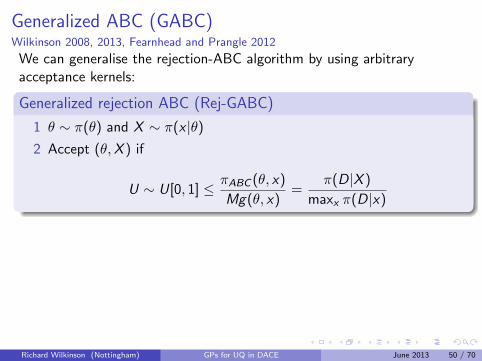
Generalized ABC (GABC)Wilkinson 2008, 2013, Fearnhead and Prangle 2012
We can generalise the rejection-ABC algorithm by using arbitraryacceptance kernels:
Generalized rejection ABC (Rej-GABC)
1 θ ∼ π(θ) and X ∼ π(x |θ)
2 Accept (θ,X ) if
U ∼ U[0, 1] ≤ πABC (θ, x)
Mg(θ, x)=
π(D|X )
maxx π(D|x)
In uniform ABC we take
π(D|X ) =
{1 if ρ(D,X ) ≤ ε0 otherwise
this reduces the algorithm to
2’ Accept θ ifF ρ(D,X ) ≤ εie, we recover the uniform ABC algorithm.
Richard Wilkinson (Nottingham) GPs for UQ in DACE June 2013 50 / 70

Generalized ABC (GABC)Wilkinson 2008, 2013, Fearnhead and Prangle 2012
We can generalise the rejection-ABC algorithm by using arbitraryacceptance kernels:
Generalized rejection ABC (Rej-GABC)
1 θ ∼ π(θ) and X ∼ π(x |θ)
2 Accept (θ,X ) if
U ∼ U[0, 1] ≤ πABC (θ, x)
Mg(θ, x)=
π(D|X )
maxx π(D|x)
In uniform ABC we take
π(D|X ) =
{1 if ρ(D,X ) ≤ ε0 otherwise
this reduces the algorithm to
2’ Accept θ ifF ρ(D,X ) ≤ εie, we recover the uniform ABC algorithm.Richard Wilkinson (Nottingham) GPs for UQ in DACE June 2013 50 / 70

Uniform ABC algorithm
This allows us to interpret uniform ABC. Suppose X ,D ∈ R
Proposition
Accepted θ from the uniform ABC algorithm (with ρ(D,X ) = |D − X |)are samples from the posterior distribution of θ given D where we assumeD = f (θ) + e and that
e ∼ U[−ε, ε]
In general, uniform ABC assumes that
D|x ∼ U{d : ρ(d , x) ≤ ε}
We can think of this as assuming a uniform error term when we relate thesimulator to the observations.
ABC gives ‘exact’ inference under a different model!
Richard Wilkinson (Nottingham) GPs for UQ in DACE June 2013 51 / 70

Problems with Monte Carlo methods
Monte Carlo methods are generally guaranteed to succeed if we run themfor long enough.
This guarantee comes at a cost.
Most methods sample naively - they don’t learn from previoussimulations.
They don’t exploit known properties of the likelihood function, suchas continuity
They sample randomly, rather than using space filling designs.
This naivety can make a full analysis infeasible without access to a largeamount of computational resource.
If we are prepared to lose the guarantee of eventual success, we canexploit the continuity of the likelihood function to learn about its shape,and to dramatically improve the efficiency of our computations.
Richard Wilkinson (Nottingham) GPs for UQ in DACE June 2013 52 / 70

Likelihood estimation
The GABC framework assumes
π(D|θ) =
∫π(D|X )π(X |θ)dX
≈ 1
N
∑π(D|Xi )
where Xi ∼ π(X |θ). Or in Wood (2010),
π(D|θ) = φ(D;µθ,Σθ)
For many problems, we believe the likelihood is continuous and smooth,so that π(D|θ) is similar to π(D|θ′) when θ − θ′ is small
We can model π(D|θ) and use the model to find the posterior in place ofrunning the simulator.
Richard Wilkinson (Nottingham) GPs for UQ in DACE June 2013 53 / 70

Example: Ricker Model
The Ricker model is one of the prototypic ecological models.
used to model the fluctuation of the observed number of animals insome population over time
It has complex dynamics and likelihood, despite its simplemathematical form.
Ricker Model
Let Nt denote the number of animals at time t.
Nt+1 = rNte−Nt +er
where et are independent N(0, σ2e ) process noise
Assume we observe counts yt where
yt ∼ Po(φNt)
Used in Wood to demonstrate the synthetic likelihood approach.
Richard Wilkinson (Nottingham) GPs for UQ in DACE June 2013 54 / 70
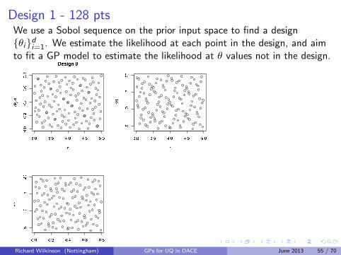
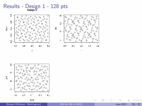
Design 1 - 128 ptsWe use a Sobol sequence on the prior input space to find a design{θi}d
i=1. We estimate the likelihood at each point in the design, and aimto fit a GP model to estimate the likelihood at θ values not in the design.
Richard Wilkinson (Nottingham) GPs for UQ in DACE June 2013 55 / 70
Difficulties
i. The likelihood is too difficult to model, so we model thelog-likelihood instead.
l̂(D|θ) = log
(1
N
∑π(D|Xi )
)ii. Use bootstrapped replicates of the log-likelihood to estimate the
variance of the nugget term (we could estimate it as part of the GPfitting, but typically this is very poorly behaved).
iii. Var(l̂(D|θ)) is far from constant as a function of θ - this causes aproblem as simple GP covariance functions assume the nugget isconstant through space.
1 Crude fix: pick a small sensible value estimated for a θ value near themode of the posterior.
Richard Wilkinson (Nottingham) GPs for UQ in DACE June 2013 56 / 70

History matching wavesThe log-likelihood varies across too wide a range of values, e.g., -10 nearthe mode, but essentially −∞ at the extremes of the prior range.Consequently, any Gaussian process model will struggle to model thelog-likelihood across the entire input range.
To fix this we introduce the idea of waves, similar to those used inMichael Goldstein’s approach to history-matching.In each wave, we build a GP model that can rule out large swathes ofspace as implausible.
We decide that θ is implausible if
m(θ) + 3σ < maxθi
log π(D|θi )− 10
where m(θ) is the Gaussian process estimate of log π(D|θ), and σ isthe variance of the GP estimate.
I We subtract 10, as for the Ricker model, a difference of 10 on the logscale between two likelihoods, means that assigning the θ with thesmaller log-likelihood a posterior density of 0 (by saying it isimplausible) is a good approximation.
Richard Wilkinson (Nottingham) GPs for UQ in DACE June 2013 57 / 70

History matching wavesThe log-likelihood varies across too wide a range of values, e.g., -10 nearthe mode, but essentially −∞ at the extremes of the prior range.Consequently, any Gaussian process model will struggle to model thelog-likelihood across the entire input range.
To fix this we introduce the idea of waves, similar to those used inMichael Goldstein’s approach to history-matching.In each wave, we build a GP model that can rule out large swathes ofspace as implausible.We decide that θ is implausible if
m(θ) + 3σ < maxθi
log π(D|θi )− 10
where m(θ) is the Gaussian process estimate of log π(D|θ), and σ isthe variance of the GP estimate.
I We subtract 10, as for the Ricker model, a difference of 10 on the logscale between two likelihoods, means that assigning the θ with thesmaller log-likelihood a posterior density of 0 (by saying it isimplausible) is a good approximation.
Richard Wilkinson (Nottingham) GPs for UQ in DACE June 2013 57 / 70
Difficulties II ctd
This still wasn’t enough in some problems, so for the first wave wemodel log(− log π(D|θ))
For the next wave, we begin by using the Gaussian processes fromthe previous waves to decide which parts of the input space areimplausible.
We then extend the design into the not-implaussible range and builda new Gaussian process
This new GP will lead to a new definition of implausibility
. . .
Richard Wilkinson (Nottingham) GPs for UQ in DACE June 2013 58 / 70
Results - Design 1 - 128 pts
Richard Wilkinson (Nottingham) GPs for UQ in DACE June 2013 59 / 70

Diagnostics for GP 1 - threshold = 5.6
Richard Wilkinson (Nottingham) GPs for UQ in DACE June 2013 60 / 70

Results - Design 2 - 314 pts - 38% of space implausible
Richard Wilkinson (Nottingham) GPs for UQ in DACE June 2013 61 / 70

Diagnostics for GP 2 - threshold = -21.8
Richard Wilkinson (Nottingham) GPs for UQ in DACE June 2013 62 / 70

Design 3 - 149 pts - 62% of space implausible
Richard Wilkinson (Nottingham) GPs for UQ in DACE June 2013 63 / 70

Diagnostics for GP 3 - threshold = -20.7
Richard Wilkinson (Nottingham) GPs for UQ in DACE June 2013 64 / 70

Design 4 - 400 pts - 95% of space implausible
Richard Wilkinson (Nottingham) GPs for UQ in DACE June 2013 65 / 70

Diagnostics for GP 4 - threshold = -16.4
Richard Wilkinson (Nottingham) GPs for UQ in DACE June 2013 66 / 70

MCMC Results
3.0 3.5 4.0 4.5 5.0
01
23
45
67
Wood’s MCMC posterior
r
Density
0.0 0.2 0.4 0.6 0.8
0.0
1.0
2.0
3.0
Green = GP posterior
sig.e
Density
5 10 15 20
0.0
0.2
0.4
Black = Wood’s MCMC
phi
Density
Richard Wilkinson (Nottingham) GPs for UQ in DACE June 2013 67 / 70
Computational details
The Wood MCMC method used 105 × 500 simulator runs
The GP code used (128 + 314 + 149 + 400) = 991× 500 simulatorruns
I 1/100th of the number used by Wood’s method.
By the final iteration, the Gaussian processes had ruled out over 98% ofthe original input space as implausible,
the MCMC sampler did not need to waste time exploring thoseregions.
Richard Wilkinson (Nottingham) GPs for UQ in DACE June 2013 68 / 70

Conclusions
Richard Wilkinson (Nottingham) GPs for UQ in DACE June 2013 69 / 70
ReferencesMUCM toolkit. www.mucm.aston.ac.uk/MUCM/MUCMToolkit
Kennedy M and O’Hagan A 2001 Bayesian calibration of computer models (withdiscussion). Journal of the Royal Statistical Society, Series B 63, 425–464.
Higdon D, Gattiker J, Williams B and Rightley M 2008 Computer modelcalibration using high-dimensional output. JASA 103, 570-583.
Oakley, J. and O’Hagan, A. (2002). Bayesian inference for the uncertaintydistribution of computer model outputs. Biometrika 89, 769-784.
Oakley, J. and O’Hagan, A. (2004). Probabilistic sensitivity analysis of complexmodels: a Bayesian approach. Journal of the Royal Statistical Society, Series B66, 751-769.
Wilkinson, Bayesian calibration of expensive multivariate computer experiments.In ‘Large-scale inverse problems and quantification of uncertainty’, 2010, Wiley.
Wilkinson, M. Vrettas, D. Cornford, J. E. Oakley, Quantifying simulatordiscrepancy in discrete-time dynamical simulators. Journal of Agricultural,Biological, and Environmental Statistics: 16(4), 554-570, 2011.
Wilkinson, Approximate Bayesian computation (ABC) gives exact results underthe assumption of model error, Statistical Applications in Genetics and MolecularBiology, 12(2), 129-142, 2013.
Wilkinson, Accelerating ABC methods using Gaussian processes. In submission.
Richard Wilkinson (Nottingham) GPs for UQ in DACE June 2013 70 / 70


