
Gender Inequality, Income, andGrowth: Are Good Times Goodfor Women?
David DollarRoberta Gatti
May 1999The World BankDevelopment Research Group/Poverty Reduction and Economic Management Network
POLICY RESEARCH REPORT ONGENDER AND DEVELOPMENTWorking Paper Series, No. 1
The PRR on Gender and Development Working Paper Series disseminates the findings of work in progress to encourage theexchange of ideas about the Policy Research Report. The papers carry the names of the authors and should be cited accordingly.The findings, interpretations, and conclusions are the author’s own and do not necessarily represent the view of the World Bank, itsBoard of Directors, or any of its member countries.Copies are available online at http: //www.worldbank.org/gender/prr.
Gender differentials in educationand health are not an efficienteconomic choice. Societies thatunderinvest in women pay aprice for it in terms of slowergrowth and lower income.Furthermore, gender inequalitycan be explained to a significantextent by religious preference,regional factors, and civilfreedom.
1
Gender Inequality, Income, and Growth:
Are Good Times Good for Women?
David Dollar and Roberta GattiDevelopment Research Group
The World Bank
Abstract
The relative status of women is poor in the developing world,compared to developed countries. Increases in per capita incomelead to improvements in different measures of gender equality,suggesting that there may be market failures hinderinginvestment in girls in developing countries, and that these aretypically overcome as development proceeds. Gender inequalityin education and health can also be explained to a considerableextent by religious preference, regional factors, and civilfreedom. These systematic patterns in gender differentialssuggest that low investment in women is not an efficienteconomic choice, and we can show that gender inequality ineducation is bad for economic growth. Thus, societies that havea preference for not investing in girls pay a price for it in termsof slower growth and reduced income.
Views expressed are those of the authors and do not necessarily reflect those of the World Bank or its membercountries. We would like to thank Bill Easterly, Beth King, Aart Kraay, Andrew Mason, and participants in aseminar at the World Bank for helpful comments, and Charles Chang for excellent research assistance.
1
If a test of civilization be sought, none can be so sure as the condition of that
half of society [women] over which the other half [men] has power.
– Harriet Martineau, “Women” (1837)
1. Introduction
Social observers have long noted that the status of women and overall socio-economic
development tend to go hand-in-hand (witness the above quote from 19th-century social critic
Harriet Martineau). In the poorest quartile of countries in 1990, only 5% of adult women had
any secondary education, one-half of the level for men. In the richest quartile, on the other
hand, 51% of adult women had at least some secondary education, 88% of the level for men.
Other measures of gender inequality (in health or legal rights) paint a similar picture. In the
poorest countries, women are particularly inadequately served in terms of education, health, or
legal rights.
What to make of this association is not obvious, however. It is possible that income
affects gender inequality; that gender inequality affects growth and hence income; or both. Or,
it may simply be that common underlying factors determine both income and gender inequality.
In this paper, we investigate the relationships among gender inequality, income, and growth,
using data for over 100 countries over the past three decades. Our primary focus is on gender
inequality in educational attainment, but it is useful to bring in other measures as well because
they reinforce our basic story.
We are interested in what macroeconomic data reveal about three specific questions:
1. Is lower investment in girls’ education simply an efficient economic choice for developing
countries?
2
2. Does gender inequality reflect different social or cultural preferences about gender roles?
and
3. Is there evidence of market failures that may lead to under-investment in girls, failures that
may decline as countries develop?
The answers to these questions are important if one is interested in reducing gender inequality.
If under-investment is efficient, then promoting girls’ education is swimming upstream. If, on
the other hand, it is not efficient for growth but reflects cultural preferences, then promoting
girls education may raise a country’s income but reduce the welfare of those who have a
preference for gender inequality. Finally, to the extent that under-investment in girls may be
the result of market failures, then a campaign to increase girls schooling could be truly “win-
win,” that is, making everyone better off.
In the next section of the paper, we develop several measures of gender inequality and
preview the data. Section 3 then considers the relevant background literature and our
methodology for addressing the above questions. In section 4, we attempt to explain the
different measures of gender inequality in terms of exogenous variables such as religious
preference, and of income (which is endogenous). Section 5 then examines the relationship in
the other direction, explaining per capita income growth in terms of exogenous factors and,
potentially, of gender inequality. The final section concludes.
We find several pieces of evidence suggesting that under-investment in girls schooling
is not simply an efficient economic choice. To a large extent, gender inequality in education
and in other areas can be explained by religious preference and underlying characteristics of
societies, such as the extent of civil liberties. These systematic relationships make it highly
unlikely that the observed inequality is economically efficient. We find further support for this
3
view in growth regressions, where an interesting and robust result is that gender inequality in
secondary education is bad for growth – but only for countries at lower middle income status
and above. From the point of view of growth, it may be that gender inequality in education is
a minor distortion at low levels of development (largely agricultural societies) and a more
significant distortion at higher levels (as societies become more industrial).
The econometric evidence suggests that societies have to pay a price for gender
inequality in terms of slower growth. However, the fact that religion variables systematically
explain differences in gender inequality suggests that some societies have a preference for
inequality and are willing to pay a price for it. (It would perhaps be more accurate to say that
those who control resources in the society have a preference for gender inequality that they are
willing to pay for.)
Finally, we find that the evidence is quite strong that increases in per capita income lead
to reductions in gender inequality. In the important area of secondary education, however, the
relationship is convex: there is little relative improvement in female attainment as countries go
from being very poor to lower middle income, and then accelerating progress as countries
move to a higher stage of development. One plausible explanation of this relationship is that
there are market failures that hinder investment in girls and that these failures diminish as
countries develop.
The basic story that emerges is that gender equality and economic development are
mutually reinforcing. Female education is a good investment that raises national income, and
higher income in turn leads to more gender equality – in education and in other areas.

4
2. Measuring Gender Inequality
There are different dimensions to gender inequality, and we consider four different
types of measures:
1. access and achievement in education (especially secondary);
2. improvement in health (as measured by gender-disaggregated life expectancy);
3. indexes of legal and economic equality of women in society and marriage; and
4. measures of women’s empowerment (percentage of women in parliament, year when
women earned the right to vote).
These different measures are positively, but not perfectly, correlated (Table 1, which
looks across countries in 1990). For example, if we take the difference between female
secondary and male secondary attainment as a measure of gender inequality, its correlation is
.35 with gender differences in life expectancy, .20 with an index of women’s legal rights in
economic matters, .28 with women’s legal rights in marriage, and -.05 with the prevalence of
women in parliament. One thing that will emerge from our analysis is that some societies can
be relatively egalitarian in one dimension (say, women’s education) but relatively unequal in
other dimensions. For this reason, it is important to look at a broad range of indicators when
considering the issue of women’s status in society.
One of the strongest empirical regularities is that all measures of gender equality are
positively correlated with per capita income. The correlations of gender measures with income
are all around .6, except for women in parliament (.43) and gender differences in secondary
education, where the correlation is a much lower .28 (Table 1). If we divide countries based on
their 1990 per capita income, the gender differences between the poorest quartile and the
richest quartile are striking (Table 2). In the poorest group, 5.4% of adult women have some

5
secondary education, compared to 11.6% of adult males.1 In the richest countries, the
comparable figures are 50.8% of women and 57.9% of men, so that the gender difference in
this case has been largely eliminated. Women live longer than men in virtually all societies, but
the difference is small in poor countries (life expectancy of 48.3 years for men and 51.3 years
for women) and large in rich countries (73.0 years for men and 79.1 years for women). In the
area of legal rights, Humana (1992) ranks countries on a scale from 1-4 for different aspects of
rights. For women’s economic rights (equal pay for equal work), the average rating is 2 for
the poorest countries and 2.9 for the richest. Differences are more striking in terms of
women’s rights within marriage, 2.3 in poor countries and 3.6 in rich ones. Similarly, the share
of parliament seats held by women averages 7% in poor countries and 17% in rich ones. The
median year in which women attained the vote was 1962 for poor countries and 1926 for rich
ones. There is little doubt that women’s freedom and overall economic development go hand-
in-hand.
The Human Development Report 1995 (p. 43) provides some concrete illustrations of
the inequality of women and men under the law in many countries:
• Right to nationality. In much of West Asia and North Africa, women married to foreigners
cannot transfer citizenship to their husbands, though men in similar situations can.
• Right to manage property. Married women are under the permanent guardianship of their
husbands and have no right to manage property in Botswana, Chile, Lesotho, Namibia, and
Swaziland.
• Right to income-earning opportunities. Husbands can restrict a wife’s employment
outside the home in Bolivia, Guatemala, and Syria.
6
• Right to travel. In some Arab countries, a husband’s consent is necessary for a wife to
obtain a passport, but not vice versa. Women cannot leave the country without their
husband’s permission in Iran.
We highlighted above that gender inequality tends to vary with income. There are also
sharp differences in gender measures across regions of the world. In educational attainment,
Latin America stands out as having relatively low attainment compared to East Asia or Europe
and Central Asia, but strikingly low gender inequality as well (Figure 1).2 South Asia, at the
other extreme, has the largest gender differential. In general, the regional patterns are similar
when it comes to gender inequality in legal rights or women in parliament (Figure 2). Europe
and Central Asia rank highly in terms of gender equality, whereas South Asia is consistently at
the bottom. The countries that make up these regions differ in terms of per capita income,
religion, and other characteristics, and one of the main objectives of the paper is to go beneath
the regional variation and understand the sources of these differences.
3. Background and Methodology
We would like to explain gender inequality across countries and over time, and also
consider the possibility that gender inequality affects growth. That is, we would like to
estimate the following equations
(1) ititit Zyg εγβα +++=
(2) itit
it
uXgyy +++=
πψδ&
where g is some measure of gender inequality;

7
y is per capita income and y
y& is per capita income growth;
Z are exogenous variables that affect gender inequality;
X are exogenous variables that affect growth;
ε and u are error terms with the usual properties.
According to the estimation technique, equations (1) and (2) might also include country-
specific fixed effects. Some of the variables in Z and X may be the same, but as long as the
variables that affect gender inequality and the variables that affect growth are not identical, we
potentially have instruments that can be used to address the problem that OLS estimates of
either (1) or (2) are likely to be biased.
There is a small macro literature that attempts to estimate either equation (1) or (2),
but before turning to a review of this previous literature, it is useful to briefly discuss the much
more extensive micro literature on gender inequality, because that literature provides some
motivation for our work. The issue of gender inequality in schooling, in particular, has drawn
a lot of attention from microeconomists.
Gertler and Alderman (1989) point out that there are three reasons why parents might
invest more in the education and health of boys than of girls. First, it may be that the return
from girls’ schooling may be lower than that for boys. This is only possible if the labor of
males and females are imperfect substitutes in some activities. In this case, different amounts
of education for girls and boys could be an efficient economic choice. A second possibility is
that the social returns to educating boys and girls are the same, but that parents expect more
direct benefit from investing in sons if, for example, sons typically provide for parents in their
old age, while daughters tend to leave and become part of a different household economic unit.

8
In this case, the wedge between private and social returns generates a market failure, and the
private decision to invest in girls’ schooling is likely to be sub-optimal. Third, parents may
simply have a preference for educating boys over girls. A low investment in girls’ education
would then reflect the underlying population preference and would not imply per se a market
failure.
The micro literature on gender can shed some light on these different possibilities,
particularly on the issue of whether or not low investment in girls is economically efficient.
Schultz (1993) points out that there are some difficulties in accurately estimating the returns to
schooling. Nevertheless, he argues that the available evidence refutes the view that low
investment in girls is economically efficient. In studies from a wide range of developing
countries, it is almost never found that the return to girls’ schooling is less than the return to
boys’ schooling (which would make less schooling for girls an efficient choice). To the
contrary, there are quite a few middle-income countries in which the estimated return to girls’
secondary schooling is far higher than the return for boys. In Thailand in 1980-81, for
example, the female return was 20.1%, compared to 11.3% for boys. In Cote d’Ivoire in
1985, the comparable figures were 28.7% and 17.0% (Schultz, 1993, p. 41). Not only are the
returns for girls higher than for boys, but the absolute value of the return is striking: the return
to girls’ education was far above real interest rates in these countries. For well-known reasons
(such as credit market imperfections), households in developing countries may be constrained
from making the optimal amount of investment in children’s human capital. But those
imperfections would affect schooling of both girls and boys and would not explain the
persistence of large gender differentials in the face of higher returns for girls than for boys.
9
Macroeconomic analysis can potentially add several things to what we have learned
from the micro literature. First, if under-investment in girls is a serious distortion, then it
should show up in the analysis of growth. Either prejudice or market failure that works against
investing in girls is analogous to a distortionary tax that reduces efficient accumulation and
leads to slower growth, which is a justification for adding measures of gender inequality to the
growth equation (2), above. Second, it is difficult to tell from the microeconomic evidence if
under-investment in girls results from market failure or if it reflects the preferences of those
who control resources and make decisions. It may be that the return to educating girls is high,
but that the adults who make decisions value gender inequality and are willing to pay a price
for it. In addressing this issue, cross-country analysis can be useful. If gender differentials in
education and health can to some extent be systematically explained by variables such as
religious preference, then it is unlikely that low investment in girls simply reflects market
failure.
There are a number of previous efforts to estimate equations (1) or (2) above. Boone
(1996) estimates a variant of (1), in which the gender measure is an index of women’s legal
rights from Humana (1992). The main finding that is relevant to our work is that religious
preference variables are useful in explaining gender inequality. Our work differs from Boone’s
in three ways: (1) we use several different measures of gender inequality; (2) we use a panel
rather than a single cross section of countries; and (3) we treat income as endogenous.
Easterly (1997) estimates a variant of (1) in which the gender measure is female to male
secondary school enrollment ratio and the only right-hand-side variable is per capita income.
In a panel with fixed effects, he shows that there is a positive relationship between income and
gender equality. Easterly’s work establishes that the correlation between income and gender

10
equality in secondary education is not simply a cross-sectional association, but in fact is true
for individual countries as they develop. Still left open, however, is the question of causality:
do increases in income actually lead to more gender equality, or is the relationship spurious?
Concerning equation (2) above, there is a large literature estimating variants of this
without reference to gender, beginning with Barro (1991). This literature attempts to explain
income growth as a function of some initial conditions, including initial per capita income, and
policies that affect the environment for accumulation. Such an equation can be derived from
either neoclassical growth theory or endogenous growth theory, the main difference being that
the former suggests that the coefficient on initial income will be negative. According to
neoclassical growth models, growth rates exhibit conditional convergence, i.e. poor countries
grow relatively rapidly after controlling for the level of steady state income. Also, in this
framework, government policies can affect growth rates only in the transition towards the
steady state, while long run growth prospects are determined solely by the rate of exogenous
technological progress. In the endogenous growth framework, instead, growth effects of
policies will be permanent. Much of the existing empirical work finds a negative coefficient on
initial income (supporting the neoclassical view). However, the size of the coefficient suggests
that the transition to the steady state is slow, so that in practice policies have effect over a
significant period of time (Barro and Sala-i-Martin 1995).
We will be starting with a growth equation using some of the variables popular in the
empirical growth literature. For our purposes, it is important to note that there is quite solid
evidence that macroeconomic stability (Fischer 1993) and trade openness (Sachs and Warner
1995) positively affect growth. Furthermore, strength of property rights and rule of law are

11
important elements of a good incentive regime (Knack and Keefer 1995). Other variables
often included in this kind of work are fertility and some measure of initial human capital.
There are only a couple of efforts to introduce measures of gender inequality into a
growth equation. Barro and Lee (1994) introduce male and female secondary attainment into
a cross-section growth regression: “A puzzling finding, which tends to recur, is that the initial
level of female secondary education enters negatively in the growth equations... One possibility
is that a high spread between male and female secondary attainment is a good measure of
backwardness; hence less female attainment signifies more backwardness and accordingly
higher growth potential through the convergence mechanism.” This explanation is not very
convincing, given that the equation already includes initial per capita income to pick up
backwardness.
Klasen (1998) finds the opposite result from Barro and Lee (1994): that growth in
female secondary attainment is positively related to per capita income growth. Both studies,
however, work mostly with a cross-section, and neither addresses the likely endogeneity of
gender differentials. Given these problems – and the fact that the two studies have opposite
results – more work in this area would seem to be called for. Moreover, studying the
determinants of gender inequality – equation (1) – should lead us to good instruments that
can be used to overcome endogeneity problems in the estimation of the growth equation.
4. Explaining Gender Inequality
We are interested in explaining gender inequality as a function of per capita income,
other characteristics such as civil liberties or economic policy, religious preference, and
regional factors. We begin with inequality in education, specifically inequality in secondary
12
attainment (the share of the adult population for which some secondary schooling is the highest
level of attainment). Table 3 presents coefficients from panel regressions where standard
errors explicitly account for heteroschedasticity and for the possible correlation of errors
within country clusters over the different periods. Our panel covers up to 127 countries and
four five-year periods (1975-79 to 1990), but there are some missing observations so we have
around 400 observations.
Although we recognize and will explicitly deal with the endogeneity issue, we start with
OLS estimates that can serve as a benchmark for useful comparison with the existing literature.
The regressions tell us which characteristics are associated with high female secondary
attainment, after controlling for the male level. We find that high female attainment is
associated with the Protestant religions and with good civil liberties, while low achievement is
weakly associated with the Muslim and Hindu religions. (The religious variables indicate the
share of the population that follows a particular religion.) There are also large positive
coefficients on the Shinto variable (virtually an indicator for Japan) and the indicator variable
for Latin America. The Latin American variable is the only regional indicator that is
significant; thus, the visible regional differences in Figure 1 can otherwise be explained by
differences in country characteristics.
In the secondary female attainment regression, per capita income enters convexly, and
strongly so. The shape of this relationship is quite interesting. It basically indicates that, as
income increases up to a level of about $2,000 per capita (PPP adjusted), there is no tendency
for female educational achievement to catch up with the superior male achievement. After that
level of income, on the other hand, there is a strong tendency to catch up. (This convex
relationship comes through clearly if you break the data set in half based on per capita income.

13
For the poorer half of the observations, there is no relationship between female attainment and
income, after controlling for male attainment. For the richer half, there is a strong, positive
relationship.)
We also introduced into the OLS regression a number of variables that are popular in
the empirical growth literature: rule of law in the economic domain and the black market
premium as a proxy for distortions in macroeconomic policy and the trade regime. Both
variables had no significance, indicating that these policies that are important for growth have
no direct effect on gender inequality in the education domain. Because both of these policy
variables are highly correlated with per capita income, they then provide us with good
instruments to address the issue of the endogeneity of per capita income. As noted, there is a
convex relationship between income and educational equality. A key question is whether we
can interpret this as a causal relationship: that increases in income actually lead to more gender
equality.
In the second column of Table 3 we instrument for per capita income and per capita
income squared, using rule of law and black market premium.3 Because of the availability of
the rule of law variable, we lose the early time periods and the number of observations is
reduced to about 200. The convex relationship between female educational achievement and
per capita income remains strong. The relationship is also there, but weaker, in fixed effects
regressions (column 3). The fixed effects regressions reveal that this is not simply a cross-
sectional effect; rather, it is fair to say that as individual countries develop, gender differences
in secondary education diminish slowly as first, and then more rapidly.
The results on secondary attainment are subject to two potential criticisms. First, our
specification explains female attainment controlling for the male level. One could alternatively

14
put the differential – female attainment minus male attainment – on the left-hand side. Second,
the secondary attainment variable captures the share of the population for whom secondary is
the highest level of attainment. One could alternatively look at the share of the population that
has at least some secondary education (secondary plus higher attainment, which we label
“superior attainment”).
In Table 4, we show that addressing these concerns does not alter the main results
concerning the relationship between income and gender differentials in secondary education.
The table shows the coefficients on the log of per capita income and that log squared, for four
different specifications and three different methodologies. In parentheses are the p-values, that
is, the probability that we can reject the hypothesis that the coefficient is zero. The first
specification repeats the coefficients from the regression of secondary female attainment,
holding male constant. The second shifts the specification to the differential of female
attainment minus male. The third changes the variable to female superior attainment. And the
fourth looks at superior differential. In each case, we have the same control variables as in
Table 3. The results for the control variables do not vary in any important way, so Table 4
focuses on the coefficients on per capita income and its square.
The convexity is clear and strong in OLS regressions for all of the specifications. In the
2SLS regressions, the relationship persists for superior attainment, but weakens for the
specifications that use the differential. Keep in mind, though, that using instruments cuts the
sample about in half because of data availability. Finally, with fixed effects, the convexity is
only strong in the specification that looks at female level controlling for the male level.
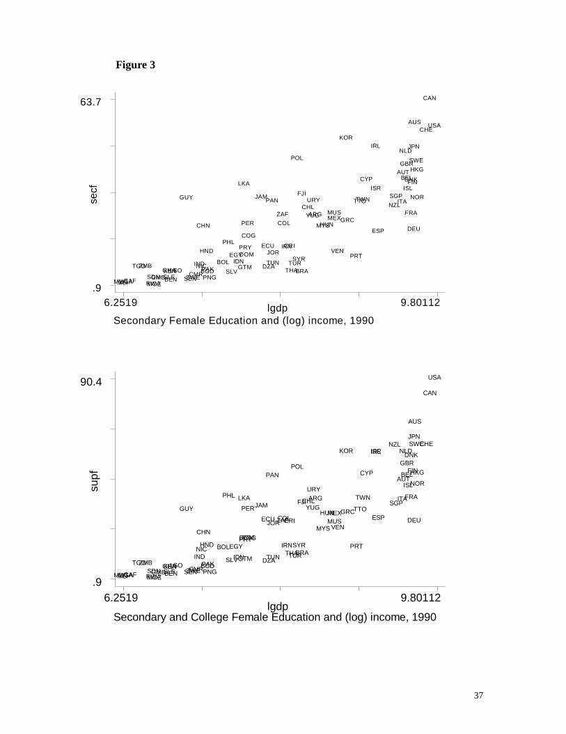
A final point about the convexity is that it is visible clearly if you simply look at the
data. Female secondary and superior attainment have sharp, convex relationships with income

15
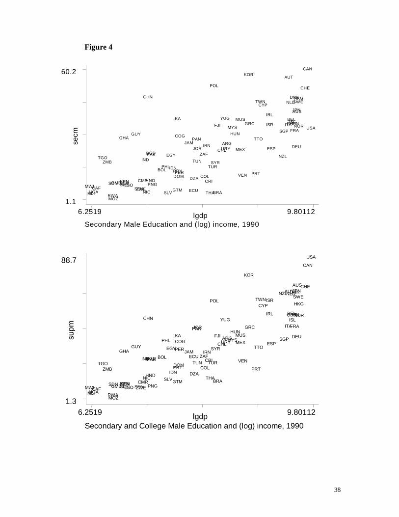
(Figure 3). The regressions show that this is true even after controlling for male attainment.
The simple relationship between male attainment and income has some convex curvature as
well, but it is much less sharp than in the case of the female (Figure 4). Figure 5 plots the
quadratic relationships between female superior attainment and log income and male superior
attainment and log income, estimated over the whole panel (with control variables). This
figure shows that there is little tendency for female attainment to catch up with male as
countries move from very poor ($500 per capita) to lower middle income ($2,000), and then a
strong tendency toward catch-up beyond that level.
To sum up the results on gender inequality in education: We find a convex relationship
between income and female achievement, after controlling for male achievement and other
variables. The fact that this relationship persists when we instrument for income provides
some confidence that this is in fact a causal relationship: increases in income lead to a
narrowing of gender inequality in education. However, the shape of the relationship means
that this effect is minor or nonexistent as countries move from very low-income to lower
middle income. The strong effect of income on educational inequality kicks in as countries
move from lower middle income to higher incomes. Furthermore, policies that have been
shown to be important for growth do not appear to directly affect inequality, though they
indirectly affect it because other work has shown that they contribute to higher per capita
income. Finally, there are differences in female achievement in education that appear to result
from regional differences, religious preferences, and the extent of civil liberties in society.
The next question that we take up is whether the patterns are similar or different when
we use other measures of gender inequality. We present both OLS (Table 5) and 2SLS
regressions (Table 6), but will confine the discussion to the latter, since they correct for the

16
potential endogeneity of income. For women’s economic equality under the law and for
women in parliament, we find the same convex relationship with income that we found for
gender differentials in education: that is, little tendency for improvement as countries go from
low-income to middle-income and then rapid improvement. Although the F-test suggests a
significant relationship between the life expectancy differential and income, it is difficult to
make inferences on its shape. Interestingly, for women’s rights in marriage we find no
significant relationship between per capita income and this measure of gender equality.
Moreover, civil liberties have no consistent relationship with any of the measures. The
Muslim religious variable has a negative coefficient in each regression, but the relationship is
only strong for equality within marriage. Shinto affiliation has a strong negative relationships
with all of these gender equality measures, except female life expectancy.
The fact that the religious variables have a considerable joint explanatory power for
these other measures of gender inequality increases our confidence that differences in cultural
preferences really are important. In general, the explanatory variables tend to have the same
sign for different measures of gender equality on the left-hand side. There are, however, some
switches in sign. The percentage of affiliates to Shinto is negatively related to all four measures
of gender equality in Table 6. Recall that this variable had instead a strong positive
relationship with female secondary attainment. By the education measure one would conclude
that Japan has relatively high status of women, whereas by these other indicators one would
conclude the opposite. Thus, one must be careful about making simple generalizations about
where the status of women is high or low – in some cases it depends on the particular
dimension of inequality that is examined.4
17
Thus, for all of these different measures of gender equality (except marriage rights), the
evidence supports the view that there is a causal relationship between per capita income and
gender equality. The policies that promote growth in per capita income will generally lead to
greater gender equality. In the case of educational achievement, economic equality, and
women in parliament, however, the convexity in the relationship indicates that this may take a
long time to play out. The other fairly robust relationship is that religious variables are good
predictors of gender inequality.
5. Gender Inequality and Growth
We turn now to the question of whether gender inequality affects growth, and here the
measure of inequality that we focus on is differential secondary school achievement. The
reason for this choice is that in the empirical growth literature it is secondary school attainment
at the beginning of a period that often is found to be a significant explainer of subsequent
growth. Furthermore, there is at least one result in the literature that finds that gender
inequality in secondary education is positively related to growth. Finally, we have from the
previous section the interesting result that per capita income appears to be a determinant of
gender equality and that for secondary educational achievement the relationship is strongly
convex.
The fact that gender inequality to a considerable extent can be explained by religious
variables, civil freedom, and regional variables, suggests that it is not simply an efficient
economic choice. In an optimizing growth model, a religious preference not to educate girls is
a distortion that can impede efficient accumulation and lead to slower growth. Similarly,
market failure could lead to under-investment in girls: the clearest example is when families
18
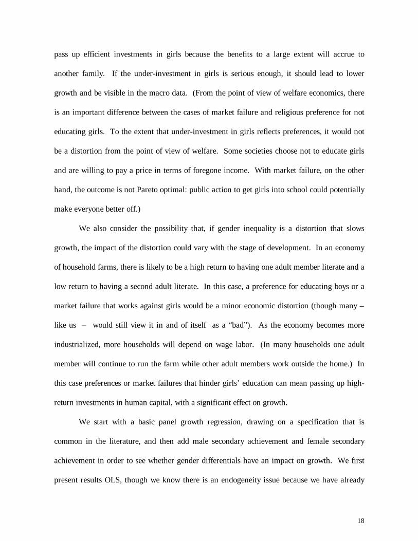
pass up efficient investments in girls because the benefits to a large extent will accrue to
another family. If the under-investment in girls is serious enough, it should lead to lower
growth and be visible in the macro data. (From the point of view of welfare economics, there
is an important difference between the cases of market failure and religious preference for not
educating girls. To the extent that under-investment in girls reflects preferences, it would not
be a distortion from the point of view of welfare. Some societies choose not to educate girls
and are willing to pay a price in terms of foregone income. With market failure, on the other
hand, the outcome is not Pareto optimal: public action to get girls into school could potentially
make everyone better off.)
We also consider the possibility that, if gender inequality is a distortion that slows
growth, the impact of the distortion could vary with the stage of development. In an economy
of household farms, there is likely to be a high return to having one adult member literate and a
low return to having a second adult literate. In this case, a preference for educating boys or a
market failure that works against girls would be a minor economic distortion (though many –
like us – would still view it in and of itself as a “bad”). As the economy becomes more
industrialized, more households will depend on wage labor. (In many households one adult
member will continue to run the farm while other adult members work outside the home.) In
this case preferences or market failures that hinder girls’ education can mean passing up high-
return investments in human capital, with a significant effect on growth.
We start with a basic panel growth regression, drawing on a specification that is
common in the literature, and then add male secondary achievement and female secondary
achievement in order to see whether gender differentials have an impact on growth. We first
present results OLS, though we know there is an endogeneity issue because we have already

19
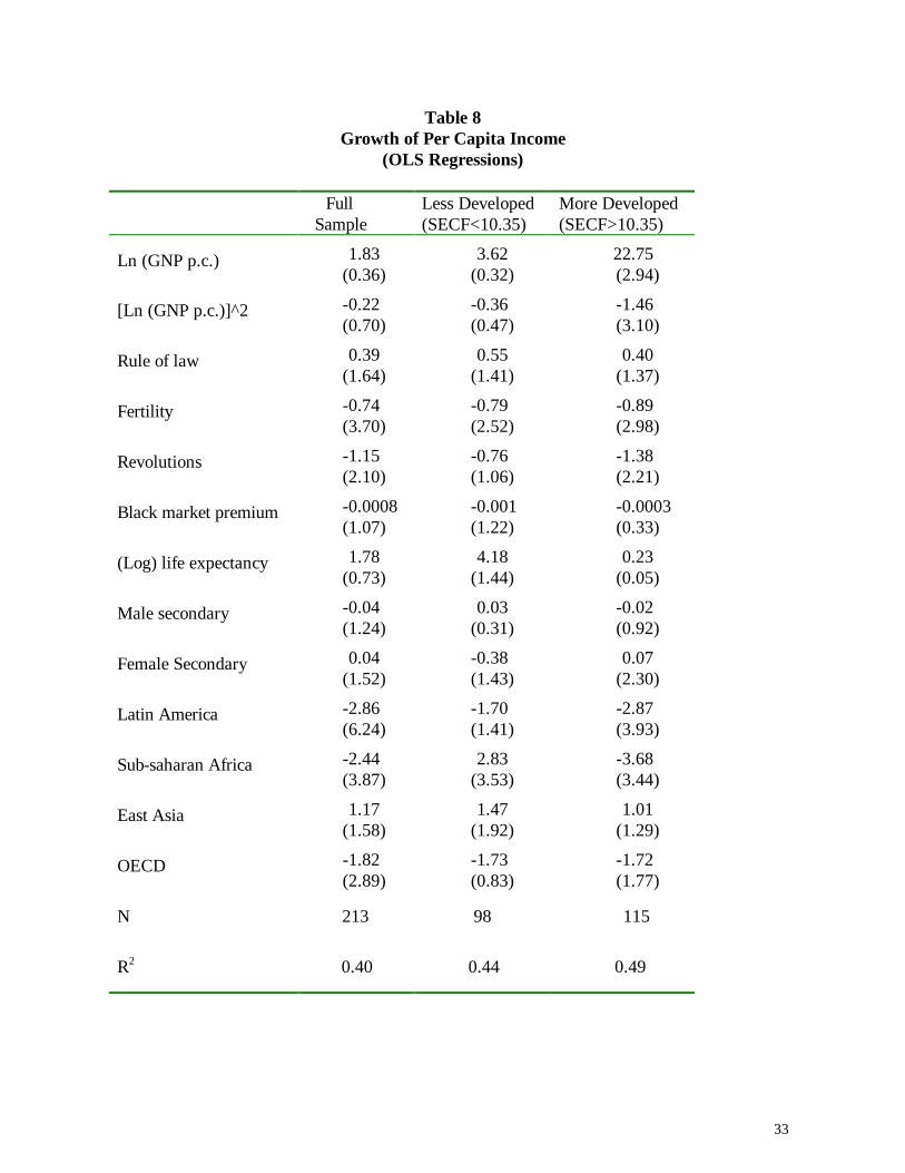
found that per capita income influences gender differentials. For the whole sample, there is a
weak negative coefficient on male education and a weak positive coefficient on female
education (Table 8). This is the opposite of what Barro and Lee (1994) found, and the
difference can primarily be explained by the presence of the regional dummies. There is a
strong tendency for Latin American economies to grow less rapidly than predicted by the other
variables, and at the same time this region has unexpectedly high female secondary
achievement. If the regional dummies are left out of the growth regression, Latin America’s
poor growth gets attributed to the female education variable.
What is interesting from the point of view of the discussion above is that the results are
quite different if the sample is divided in half on the basis of female secondary school
achievement. For less developed economies (with secondary female attainment covering less
than 10.35% of the population), there are insignificant coefficients on both male and female
secondary attainment. For the more developed economies in the sample, there is a modestly
negative coefficient on male education and a significant positive coefficient on female
secondary attainment. As in much other work, there is also a large, negative coefficient on
fertility. Female education may well contribute to per capita income growth by reducing
fertility and hence population growth. We, however, are interested in the direct effect of
gender discrimination on growth, after controlling for fertility.
The work in the previous section provides us with good instruments for addressing the
endogeneity of gender differentials. In particular, we argue that the religion variables and civil
liberties belong in the gender equations but not in the growth equation, so that we can use
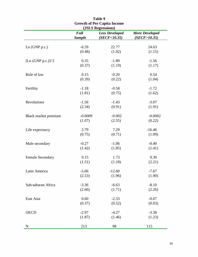
them as instruments for male education and female education.5 The results of the 2SLS
regressions confirm the pattern highlighted by the OLS estimation (Table 9). For the more
20
developed half of the sample, there remains a negative coefficient on male secondary
attainment and a significant positive coefficient on female attainment. The order of magnitude
of the coefficient also suggests that secondary female education has an economically significant
impact on growth: in the countries with higher initial education, an increase of 1 percentage
point in the share of adult women with secondary school education implies an increase in per
capita income growth of 0.3 percentage points.
6. Conclusions
It is a fair generalization to say that the relative status of women is poor in the
developing world, compared to developed countries. In the poorest countries, as a rule, girls
get less education than boys, there is less investment in women’s health than in men’s, legal
rights of women in the economy and in marriage are weaker than men’s rights, and women
have less political power (as evidenced, for example, by their low representation in
parliaments).
We treat gender inequality as an endogenous variable and show that it can be explained
to a considerable extent by religious preference, regional factors, and civil freedom. For some
of these variables, the direction of the effect depends on the particular measure of inequality.
For example, the Shinto religion is associated with high female educational attainment and low
status of women in other dimensions. In general, however, the same variables that predict low
status of women in one dimension, do so in others. Thus, affiliations to Muslim and Hindu
religions are consistently associated with high gender inequality, whereas the Protestant
religion and high civil liberties are associated with low inequality. The fact that these variables

21
systematically explain gender differentials in education and health suggests that low investment
in women’s human capital is not simply an efficient economic choice for developing countries.
A second main finding is that gender inequality in education is bad for economic
growth. In the more developed half of our data set, a robust result is that there is a significant
positive coefficient on female secondary attainment and an insignificant negative one on male
attainment. The result holds up when we instrument for education with the religion variables
and civil liberties. The result suggests that an exogenous increase in girls’ access to education
creates a better environment for economic growth and that the result is particularly strong for
middle income countries. Thus, societies that have a preference for not investing in girls pay a
price for it in terms of slower growth and reduced income.
A third result is that there is strong and consistent evidence that increases in per capita
income lead to improvements in different measures of gender equality. To answer the question
in our subtitle, apparently good times are good for women. The implication of this finding is
not that growth is all that is needed to eliminate gender inequality. The findings on religious
variables, regional effects, and civil liberties suggest that there is considerable scope for direct
action on gender issues. However, it is important to know that the country-wide policies that
support rapid growth are also indirectly contributing to gender equality. Some literature has
raised the concern that growth-enhancing policies are bad for women; the evidence quite
strongly supports the opposite view. It is somewhat sobering, however, that for the important
issue of female education, the relationship between income and female attainment is convex:
that is, there is little relative improvement as societies move from being extremely poor to
being lower-middle income, and then rapid relative improvement as societies move to a more
developed stage.
22
Finally, we can relate these findings back to our three main questions:
1. Is lower investment in girls’ education simply an efficient economic choice for developing
countries? No. Countries that under-invest grow more slowly.
2. Does gender inequality reflect different social or cultural preferences about gender roles?
Yes. To some extent under-investment in girls reflects societal preferences, and in these cases
exogenous increases in girls schooling are likely to make some people worse off.
3. Is there evidence of market failures that may lead to under-investment in girls, failures that
may decline as countries develop? This is the hardest question to answer at this point. The
fact that increases in income lead to lower gender inequality suggests that there may be market
failures that hinder investment in girls in developing countries and that these are typically
overcome as development proceeds. In particular, as pension systems and capital markets
more broadly develop, parents may not need to rely so strongly on sons’ support for their
retirement, which would reduce a bias in favor of male education. An important area for future
research is to investigate whether the impact of income on gender inequality is partly through
an effect of income on capital market development.

23
References
Banks, Arthur (1995). Cross-National Time-Series Data Archive, State University of New
York at Binghamton.
Barro, Robert (1991). “Economic Growth in a Cross Section of Countries,” Quarterly Journal
of Economics, May, (106): 407-43.
Barro, Robert and Jong-Wha Lee (1993). “International Comparisons of Educational
Attainment,” Journal of Monetary Economics, December, (32): 363-394.
(1994). “Sources of Economic Growth,” Carnegie–Rochester
Conference Series on Public Policy, (40): 1-46.
Barro, Robert and Xavier Sala-i-Martin (1995). Economic Growth, McGraw-Hill, New York.
Boone, Peter (1996). “Political and Gender Oppression as a Cause of Poverty,” Manuscript,
London School of Economics.
Easterly, William (1997). “Life During Growth,” Manuscript, The World Bank.
Fischer, Stanley (1993). “The Role of Macroeconomic Factors in Growth,” Journal of
Monetary Economics, December, (32): 485-512.
Gertler, Paul and Harold Alderman (1989). “Family resources and Gender Differences in
Human Capital Investments,” paper presented at the conference on “The Family, Gender
Differences and Development,” Economic Growth Center, Yale University.

24
Humana, Charles (1992). World Human Rights Guide, Oxford University Press, New York,
3rd ed.
Klasen, Stephen (1998). “Gender inequality and Growth in Sub-Saharan Africa: Some
Preliminary Findings,” Manuscript, University of Munich.
Knack, Stephen and Philip Keefer (1995). “Institutions and Economic Performance: Cross-
Country Tests Using Alternative Institutional Measures,” Economics and Politics, November,
(3): 207-27.
Sachs, Jeffrey and Andrew Warner (1995). “Economic Reform and the Process of Global
Integration,” Brookings Papers on Economic Activity, (1): 1-118.
Schultz, T. Paul (1993). “Investment in the Schooling and Health of Women and Men;
Quantities and Returns,” Economic Growth Center Discussion Paper (702), Yale University.
United Nations Development Programme, Human Development Report 1995, New York:
Oxford U. Press.

25
Data Appendix
CIVIL LIBERTIES Gastil index of civil liberties. Values from 1 to 7, (7=mostfreedom) are attributed to countries taking intoconsideration such issues as freedom of press, of politicalassociation and trade unions. The index is available for theyears 1972-95. Source: Banks.
GDP Real GDP per capita in constant dollars, chain Indexdeflated, expressed in international prices, base 1985.Source: Summers-Heston, years 1960-1990.
LIFE EXPECTANCY Years of life expectancy at birth, female and male;indicates the number of years a newborn infant would liveif prevailing patterns of mortality at the time of its birthwere to stay the same throughout its life. Source: WDI,World Bank.
SECONDARY SCHOOL Percentage of female or male population over 25 forATTAINMENT whom primary (secondary) school education is the highest
level of education attained. Source: Barro-Lee (1993).
RELIGIOUS AFFILIATION Percentage of population who professes a religion. Source:Barrett (1982).
RULE of LAW Law and order tradition, index ranging from 0 to 6, (worstto best) Source: International Country Risk Guide, years1982, 1985, 1990.
WOMEN IN PARLIAMENT Percentage of seats occupied by women in the lower andupper chamber. Source: WISTAT.
WOMEN ECONOMIC RIGHTS Women and men are entitled to equal pay for equal work.Source: Humana (1992).
WOMEN RIGHTS WITHIN Equality of sexes within marriage and divorceMARRIAGE proceedings. Source: Humana (1992).
VOTE TO WOMEN Year when the right to vote was extended to women.Source: WISTAT.

26
Table 1Correlations Among Gender Measures and Per Capita Income
80 Countries (1990)
Income Secondary Life Economic Marriage
Per Capita Income
Secondary Ed. Differentiala 0.28
Life Exp. Differentialb 0.61 0.35
Women’s Economic Rights 0.60 0.20 0.58
Women’s Marriage Rights 0.64 0.28 0.71 0.66
Women in Parliament 0.43 -0.05 0.27 0.4 0.43
a Female secondary attainment minus male secondary attainmentb Female life expectancy minus male life expectancy

27
Table 2Gender Measures for the Poorest and Richest Quantiles of Countries
(1990)
Poorest(y<1182)
Richest(y>7478)
Female Secondary Attainment 5.0 37.7
Male Secondary Attainment 10.4 38.7
Female Superior Attainment 5.4 50.8
Male Superior Attainment 11.6 57.9
Female Life Expectancy 51.3 79.1
Male Life Expectancy 48.3 73.0
Women’s Economic Rights (1-4) 2.0 2.9
Women’s Marriage Rights (1-4) 2.3 3.6
Women in Parliament(% seats held in the lower chamber)
7 17
Year women were allowed to vote 1962 1926

28
Table 3Explaining female secondary attainment
(1)OLS
(2)2SLS
(3)Fixed Effects
Male level 0.70(11)
0.73(8.95)
0.69(26.24)
Ln (GNP p.c.) -21.3(2.52)
-77.8(2.19)
-10.28(1.35)
[Ln (GNP p.c.)]^2 1.54(2.78)
4.93(2.31)
0.73(1.54)
Civil Liberties 0.31(1.64)
0.52(1.00)
0.07(0.42)
Muslim -0.02(1.46)
-0.04(1.42)
-0.70(2.05)
Roman Catholic 0.00(0.20)
-0.04(1.21)
-0.07(0.51)
Other Christian 0.19(2.84)
0.06(0.41)
0.12(0.40)
Hindu -0.02(1.10)
-0.14(2.37)
0.29(0.54)
Shinto 2.51(5.47)
2.44(2.91)
-0.64(0.25)
Latin America 4.37(2.78)
6.79(2.66)
--
Sub-Saharan Africa 1.04(0.78)
-7.49(1.36)
--
East Asia 0.31(0.20)
0.25(0.10)
--
OECD 1.79(1.05)
-2.93(1.04)
--
N 392 211 392
R2 0.91 * 0.82*R2 is not a good measure of fitness in 2SLS estimation. Instruments are rule of lawindex and black market premium, each entered linearly and quadratically. P-value fortest of over-identifying restriction is 0.63. t-statistics in parentheses.

29
Table 4Different Specifications for Education Differentials
OLS 2SLS FixedEffects
Secondary Female Attainmenta
(log) per capita GDP -21.3(0.01)
-77.8(0.02)
-10.3(0.18)
(log) per capita GDP squared 1.55(0.01)
4.93(0.02)
0.73(0.13)
Secondary Differentialb
(log) per capita income -17.0(0.03)
-42.3(0.26)
-2.22(0.81)
(log) per capita income squared 1.14(0.02)
2.68(0.23)
0.15(0.80)
Superior Female Attainmenta
(log) per capita income -24.5(0.00)
-56.7(0.14)
-11.2(0.16)
(log) per capita income squared 1.68(0.00)
3.6(0.13)
0.75(0.13)
Superior Differentialb
(log) per capita income -17.6(0.02)
-22.0(0.56)
-3.69(0.67)
(log) per capita income squared 1.11(0.02)
1.42(0.53)
0.21(0.70)
a Controlling for the male levelb Female level minus the male levelNote: P-values in parentheses.

30
Table 5Other Measures of Gender Inequality
(OLS Regressions)
Life Expectancy EconomicEquality
Equality inMarriage
Women inParliament
Male Level 1.02(40)
-- -- --
Ln (GNP p.c.) 0.99(5.16)
0.23(2.3)
0.84(0.67)
-0.16(1.3)
[Ln (GNP p.c.)]^2 -- -- -0.04(0.59)
0.01(1.36)
Civil Liberties -0.08(1.07)
0.013(0.33)
-0.06(1.12)
-0.009(2.23)
Muslim -0.01(3.46)
-0.006(3.13)
-0.01(5.14)
-0.0008(3.18)
Roman Catholic 0.001(0.39)
-0.001(0.55)
-0.005(1.61)
-0.0006(2.25)
Other Christian -0.01(1.47)
0.0007(0.50)
-0.0004(0.08)
-0.001(1.42)
Hindu -0.02(1.97)
-0.005(1.83)
-0.009(2.09)
0.0001(0.25)
Shinto -0.2(2.22)
-0.34(15.58)
-0.30(6.85)
-0.031(3.58)
N 495 159 159 266
R2 0.99 0.59 0.51 0.28

31
Table 6Other measures of gender inequality
(2SLS regressions)
Life Expectancy EconomicEquality
Equality inMarriage
Women inParliament
Male Level 1.02(8.8)
-- -- --
Ln (GNP p.c.) -6.61(0.42)
-3.36(2.06)
-0.66(0.16)
-1.38(2.49)
[Ln (GNP p.c.)]^2 0.46(0.53)
0.24(2.23)
0.04(0.20)
0.08(2.5)
Civil Liberties -0.05(0.31)
0.01(0.21)
-0.02(0.26)
-0.003(0.34)
Muslim -0.006(0.87)
0.001(0.72)
-0.008(2.57)
-0.0002(0.56)
Roman Catholic -0.001(0.31)
0.001(0.67)
-0.004(1.39)
-0.001(2.12)
Other Christian -0.002(0.03)
-0.0005(0.04)
0.008(0.45)
-0.003(1.52)
Hindu -0.02(1.43)
0.002(0.55)
-0.002(0.41)
0.0002(0.17)
Shinto -0.32(1.87)
-0.35(6.89)
-0.32(6.16)
-0.05(3.5)
N 235 130 129 129
P-value for F test on income 0.01 0.02 0.79 0.04
P-value for OIR test 0.33 0.71 0.13 0.32

32
Table 7Other Measures of Gender Inequality
(Fixed Effects Regressions)
Life Expectancy EconomicEquality
Equality inMarriage
Women inParliament
Male Level 0.99(32.1)
-- -- --
Ln (GNP p.c.) 0.67(0.2)
3.42(1.18)
-2.96(0.49)
-0.54(3.27)
[Ln (GNP p.c.)]^2 -0.03(0.14)
-0.18(-1.09)
0.22(0.62)
0.03(3.52)
Civil Liberties 0.12(1.57)
0.009(0.22)
-0.05(0.63)
-0.009(2.31)
Muslim -0.18(0.17)
-- -- 0.02(2.47)
Roman Catholic -0.86(0.82)
-- -- -0.005(1.65)
Other Christian -4.89(0.67)
-- -- -0.015(2.52)
Hindu -0.47(0.27) -- -- 0.02
(2.07)
Shinto -0.53(0.54)
-- -- -0.031(3.58)
N 495 159 159 266
R2 within 0.99 0.04 0.17 0.32
33
Table 8Growth of Per Capita Income
(OLS Regressions)
Full Sample
Less Developed(SECF<10.35)
More Developed(SECF>10.35)
Ln (GNP p.c.) 1.83(0.36)
3.62(0.32)
22.75(2.94)
[Ln (GNP p.c.)]^2 -0.22(0.70)
-0.36(0.47)
-1.46(3.10)
Rule of law 0.39(1.64)
0.55(1.41)
0.40(1.37)
Fertility -0.74(3.70)
-0.79(2.52)
-0.89(2.98)
Revolutions -1.15(2.10)
-0.76(1.06)
-1.38(2.21)
Black market premium -0.0008(1.07)
-0.001(1.22)
-0.0003(0.33)
(Log) life expectancy 1.78(0.73)
4.18(1.44)
0.23(0.05)
Male secondary -0.04(1.24)
0.03(0.31)
-0.02(0.92)
Female Secondary 0.04(1.52)
-0.38(1.43)
0.07(2.30)
Latin America -2.86(6.24)
-1.70(1.41)
-2.87(3.93)
Sub-saharan Africa -2.44(3.87)
2.83(3.53)
-3.68(3.44)
East Asia 1.17(1.58)
1.47(1.92)
1.01(1.29)
OECD -1.82(2.89)
-1.73(0.83)
-1.72(1.77)
N 213 98 115
R2 0.40 0.44 0.49
34
Table 9Growth of Per Capita Income
(2SLS Regressions) Full Sample
Less Developed(SECF<10.35)
More Developed(SECF>10.35)
Ln (GNP p.c.) -6.59(0.48)
22.77(1.02)
24.63(1.15)
[Ln (GNP p.c.)]^2 0.35(0.37)
-1.89(1.19)
-1.56(1.17)
Rule of law 0.15(0.39)
-0.20(0.22)
0.54(1.04)
Fertility -1.18(1.81)
-0.58(0.75)
-1.72(1.62)
Revolutions -1.56(2.34)
-1.43(0.91)
-3.07(1.91)
Black market premium -0.0009(1.07)
-0.002(2.55)
-0.0002(0.22)
Life expectancy 2.79(0.75)
7.29(0.71)
-16.46(1.09)
Male secondary -0.27(1.42)
-1.06(1.85)
-0.40(1.41)
Female Secondary 0.15(1.51)
1.73(1.18)
0.30(2.21)
Latin America -5.06(2.53)
-12.60(1.96)
-7.67(1.90)
Sub-saharan Africa -3.36(2.66)
-6.63(1.71)
-8.10(2.26)
East Asia 0.60(0.37)
-2.33(0.52)
-0.07(0.03)
OECD -2.97(1.87)
-4.27(1.46)
-3.38(1.23)
N 213 98 115

35
Figure 1. Educational Attainment - Secondary and Higher by Region (%)
0
5
10
15
20
25
30
35
40
45
50
East Asia & Pacific Europe & CentralAsia
Latin America &Carribean
Middle East & NorthAfrica
South Asia Sub-Saharan Africa
Male Educational Attainment - Secondary and Higher
Female Educational Attainment - Secondary and Higher

36
Figure 2
Women in Parliament (%)
1
6
11
16
21
East Asia &Pacific
Europe &Central
Asia
LatinAmerica &Carribean
Middle East& NorthAfrica
South Asia Sub-Saharan
Africa
Women's Economic Rights
1.0
1.5
2.0
2.5
3.0
3.5
East Asia &Pacific
Europe &Central Asia
LatinAmerica &Carribean
Middle East& NorthAfrica
South Asia Sub-Saharan
Africa
Women's Marriage Rights
1.0
1.5
2.0
2.5
3.0
3.5
4.0
East Asia &Pacific
Europe &Central
Asia
LatinAmerica &Carribean
M iddle East& NorthAfrica
South Asia Sub-Saharan
Africa
37
Figure 3
supf
Secondary and College Female Education and (log) income, 1990lgdp
6.2519 9.80112.9
90.4
DZA
ARG
AUS
AUT
BGD
BEL
BEN
BOLBRA
CMR
CAN
CAF
CHL
CHN
COL
COG
CRI
CYP
DNK
DOM
ECU
EGY
SLV
FJI
FIN
FRA
GMB
DEU
GHA
GRC
GTM
GUY
HND
HKG
HUN
ISL
IND IDN
IRN
IRLISR
ITAJAM
JPN
JOR
KEN
KOR
LSOMWI
MYS
MLI
MUSMEX
MOZ
NLDNZL
NIC
NOR
PAK
PAN
PNG
PRY
PER
PHL
POL
PRT
RWASENSLE
SGP
ZAF ESP
LKA
SDN
SWECHE
SYRTHA
TGO
TTO
TUN TUR
UGA
GBR
USA
URY
VEN
YUG
ZMBZWE
TWN
secf
Secondary Female Education and (log) income, 1990lgdp6.2519 9.80112
.9
63.7
DZA
ARG
AUS
AUT
BGD
BEL
BEN
BOLBRACMR
CAN
CAF
CHL
CHN COL
COG
CRI
CYP DNK
DOMECU
EGY
SLV
FJI
FIN
FRA
GMB
DEU
GHA
GRC
GTM
GUY
HND
HKG
HUN
ISL
IND IDN
IRN
IRL
ISR
ITAJAM
JPN
JOR
KEN
KOR
LSO
MWI
MYS
MLI
MUSMEX
MOZ
NLD
NZL
NIC
NOR
PAK
PAN
PNG
PRY
PER
PHL
POL
PRT
RWASENSLE
SGP
ZAF
ESP
LKA
SDN
SWE
CHE
SYR
THATGO
TTO
TUN TUR
UGA
GBR
USA
URY
VEN
YUG
ZMB
ZWE
TWN
38
Figure 4
supm
Secondary and College Male Education and (log) income, 1990lgdp6.2519 9.80112
1.3
88.7
DZA
ARG
AUSAUT
BGD
BEL
BEN
BOL
BRACMR
CAN
CAF
CHL
CHN
COL
COG
CRI
CYP
DNK
DOM
ECU
EGY
SLV
FJI
FIN
FRA
GMB
DEU
GHA
GRC
GTM
GUY
HND
HKG
HUN
ISL
IND
IDN
IRN
IRL
ISR
ITA
JAM
JPN
JOR
KEN
KOR
LSOMWI
MYS
MLI
MUS
MEX
MOZ
NLDNZL
NIC
NOR
PAK
PAN
PNG
PRY
PER
PHL
POL
PRT
RWA
SENSLE
SGP
ZAF
ESP
LKA
SDN
SWE
CHE
SYR
THA
TGO
TTO
TUN TUR
UGA
GBR
USA
URY
VEN
YUG
ZMB
ZWE
TWN
secm
Secondary Male Education and (log) income, 1990lgdp6.2519 9.80112
1.1
60.2
DZA
ARG
AUS
AUT
BGD
BEL
BEN
BOL
BRA
CMR
CAN
CAF
CHL
CHN
COL
COG
CRI
CYP
DNK
DOM
ECU
EGY
SLV
FJI FIN
FRA
GMB
DEU
GHA
GRC
GTM
GUY
HND
HKG
HUN
ISL
IND
IDN
IRN
IRL
ISR ITA
JAM
JPN
JOR
KEN
KOR
LSOMWI
MYS
MLI
MUS
MEX
MOZ
NLD
NZL
NIC
NOR
PAK
PAN
PNG
PRYPERPHL
POL
PRT
RWA
SENSLE
SGP
ZAFESP
LKA
SDN
SWE
CHE
SYR
THA
TGO
TTO
TUNTUR
UGA
GBRUSA
URY
VEN
YUG
ZMB
ZWE
TWN

39
Figure 5. Educational Attainment (Secondary and Higher) and Per CapitaIncome
0
10
20
30
40
50
60
70
80
6.5 7 7.5 8 8.5 9 9.5 10 10.5
Per Capita GNP (Log Scale)
Sec
onda
ry A
ttai
nmen
tA
ttai
nmen
t(%
of A
dult
Pop
ulat
ion)
Male
Female

40
1 We are going to work with two education variables. Secondary attainment is the share of the adult populationfor whom some secondary education is the highest level of attainment. Secondary or higher attainment adds tothis the share of the population for whom some higher education is the highest level of attainment.2 The regional classification of countries is that used by the World Bank. The OECD countries have beenexcluded from the figure, so that the focus is on developing countries of different regions.3 The test of over-identifying restrictions indicates that these are valid instruments.4 In Table 7 we present fixed-effects regressions. The convex relationship with income remains strong for womenin parliament. That it disappears for life expectancy differential and economic equality indicates that the resultsfor those measures come primarily from the cross-section information. Nevertheless, because we have good andvalid instruments we feel confident making inferences from the 2SLS regressions.5 The test of over-identifying restrictions indicates that these are valid instruments.


