
GENERALIZED LINEAR MODELS WITH REGULARIZATION
A DISSERTATION
SUBMITTED TO THE DEPARTMENT OF STATISTICS
AND THE COMMITTEE ON GRADUATE STUDIES
OF STANFORD UNIVERSITY
IN PARTIAL FULFILLMENT OF THE REQUIREMENTS
FOR THE DEGREE OF
DOCTOR OF PHILOSOPHY
Mee Young Park
September 2006

c© Copyright by Mee Young Park 2006
All Rights Reserved
ii

I certify that I have read this dissertation and that, in my opinion, it
is fully adequate in scope and quality as a dissertation for the degree
of Doctor of Philosophy.
Trevor Hastie Principal Adviser
I certify that I have read this dissertation and that, in my opinion, it
is fully adequate in scope and quality as a dissertation for the degree
of Doctor of Philosophy.
Art Owen
I certify that I have read this dissertation and that, in my opinion, it
is fully adequate in scope and quality as a dissertation for the degree
of Doctor of Philosophy.
Robert Tibshirani
Approved for the University Committee on Graduate Studies.
iii

Abstract
Penalizing the size of the coefficients is a common strategy for robust modeling in re-
gression/classification with high-dimensional data. This thesis examines the properties
of the L2 norm and the L1 norm constraints applied to the coefficients in generalized
linear models (GLM).
In the first part of the thesis, we propose fitting logistic regression with a quadratic
penalization on the coefficients for a specific application of modeling gene-interactions.
Logistic regression is traditionally a popular way to model a binary response variable;
however, it has been criticized due to a difficulty of estimating a large number of param-
eters with a small number of samples, which is a typical situation in gene-interaction
models. We show that the slight modification of adding an L2 norm constraint to
logistic regression makes it possible to handle such data and yields reasonable predic-
tion performance. We implement it in conjunction with a forward stepwise variable
selection procedure.
We also study generalized linear models with an L1 norm constraint on the coeffi-
cients, focusing on the regularization path algorithm. The L1 norm constraint yields a
sparse fit, and different sets of variables are selected according to the level of regular-
ization; therefore, it is meaningful to track how the active set changes along the path
and to choose the optimal model complexity. Following the idea of the Lars-Lasso
path proposed by Efron, Hastie, Johnstone & Tibshirani (2004), we generalize the
iv

algorithm to the piecewise smooth coefficient paths for GLM. We use the predictor-
corrector scheme to trace the nonlinear path. Furthermore, we extend our procedure
to fit the Cox proportional hazards model, again penalizing the L1 norm of the coef-
ficients.
For the final part of the thesis, having studied the forward stepwise variable se-
lection procedure with L2 penalized logistic regression and the L1 regularization path
algorithm for GLM, we then merge these two earlier approaches. That is, we con-
sider several regularization path algorithms with grouped variable selection for gene-
interaction models, as we have fit with stepwise logistic regression. We examine group-
Lars/group-Lasso introduced in Yuan & Lin (2006) and also propose a new version
of group-Lars. All these regularization methods with an automatic grouped variable
selection are compared to our stepwise logistic regression scheme, which selects groups
of variables in a greedy manner.
v

Acknowledgments
Throughout my degree, I have received tremendous support from Professor Trevor
Hastie, my adviser. His insights regarding both scholarly and practical matters in
statistics have always encouraged me to take the next step to becoming a statistician.
I have been very privileged to have him as an adviser who is not only enthusiastic and
caring, but also friendly. When my parents visited Stanford, and my Dad came by his
office, he, too, was impressed by Professor Hastie’s hospitality and sense of humor. I
also want to thank his family for the warm welcomes I received whenever I was invited
to his home.
I am grateful to Professor Robert Tibshirani for always listening to me attentively
at our weekly group meetings and providing invaluable comments. His distinctive and
timely input often enabled me to gain a new perspective on the various problems I
encountered. I also thank Professor Art Owen for encouraging me in my job search
and for reading my thesis very thoroughly.
Particular thanks go to Professor Bradley Efron and Professor Jerome Friedman.
At my defense, they did not simply test me, but also gave me priceless advice for my
future research. All the committee members eased my anxiety throughout my defense,
and when they told me that I had passed my oral exams, it made my day.
I am pleased to have had all my statistics buddies in Sequoia Hall. I appreciate all
the members of the Hastie-Tibshirani group meeting for their input and for the fun
times we shared, including the gathering at JSM 2006. I thank all of my peers who
vi

came to the department in the same year as I did, for the enjoyable memories - from
a late night HW discussion to dining out.
I would like to thank all my Korean friends at Stanford. Many of them taught
me that I can share true friendship with people of any age. Because of their support,
I have moved along my path feeling entertained rather than exhausted. I especially
thank my KCF (Korean Christian Fellowship) family, who are faithful and lovely.
Their presence and their prayers helped me to grow spiritually, and made my life at
Stanford fruitful. They have gifted me with experiences and sharing that I never could
have received from anyone else.
I wish to express my deepest gratitude to all my mentors and friends in Korea.
Whenever I visited Korea during my academic breaks, my undergraduate mentors at
Seoul National University fed me with kind encouragement and wisdom. My dear
friends in Korea have always been my sustenance - our heartwarming conversations
let me come back to the United States energized and refreshed, every time.
This dissertation is dedicated to my parents who taught me how to eat. I owe
them much more than I can express. Throughout the years in which I have studied
in the US, they have always guided me, both emotionally and intellectually. I honor
my Dad’s positive attitude and my Mom’s sparkling and warm personality. I thank
my only brother for always being there, unchanged in every circumstance. I am sorry
that I could not attend your wedding because of the visa issue, at this time that I
am completing my thesis. But I want to see you happy forever and ever. My family
enabled me to do all that I have done, just by being beside me.
Finally, I thank God for all His blessings, to the very best of my ability.
vii

Contents
Abstract iv
Acknowledgments vi
1 Introduction 1
1.1 Fitting with High-dimensional Data . . . . . . . . . . . . . . . . . . . . 1
1.1.1 Genotype measurement data . . . . . . . . . . . . . . . . . . . . 1
1.1.2 Microarray gene expression data . . . . . . . . . . . . . . . . . . 2
1.2 Regularization Methods . . . . . . . . . . . . . . . . . . . . . . . . . . 3
1.2.1 L2 regularization . . . . . . . . . . . . . . . . . . . . . . . . . . 3
1.2.2 L1 regularization . . . . . . . . . . . . . . . . . . . . . . . . . . 4
1.2.3 Grouped L1 regularization . . . . . . . . . . . . . . . . . . . . . 5
1.3 Outline of the Thesis . . . . . . . . . . . . . . . . . . . . . . . . . . . . 6
2 Penalized Logistic Regression 8
2.1 Background . . . . . . . . . . . . . . . . . . . . . . . . . . . . . . . . . 9
2.2 Related Work . . . . . . . . . . . . . . . . . . . . . . . . . . . . . . . . 10
2.2.1 Multifactor dimensionality reduction . . . . . . . . . . . . . . . 10
2.2.2 Conditional logistic regression . . . . . . . . . . . . . . . . . . . 15
2.2.3 FlexTree . . . . . . . . . . . . . . . . . . . . . . . . . . . . . . . 17
viii

2.3 Penalized Logistic Regression . . . . . . . . . . . . . . . . . . . . . . . 18
2.3.1 Advantages of quadratic penalization . . . . . . . . . . . . . . . 20
2.3.2 Variable selection . . . . . . . . . . . . . . . . . . . . . . . . . . 23
2.3.3 Choosing the regularization parameter λ . . . . . . . . . . . . . 24
2.3.4 Missing value imputation . . . . . . . . . . . . . . . . . . . . . . 26
2.4 Simulation Study . . . . . . . . . . . . . . . . . . . . . . . . . . . . . . 27
2.5 Real Data Example . . . . . . . . . . . . . . . . . . . . . . . . . . . . . 30
2.5.1 Hypertension dataset . . . . . . . . . . . . . . . . . . . . . . . . 30
2.5.2 Bladder cancer dataset . . . . . . . . . . . . . . . . . . . . . . . 35
2.6 Summary . . . . . . . . . . . . . . . . . . . . . . . . . . . . . . . . . . 38
3 L1 Regularization Path Algorithm 41
3.1 Background . . . . . . . . . . . . . . . . . . . . . . . . . . . . . . . . . 41
3.2 GLM Path Algorithm . . . . . . . . . . . . . . . . . . . . . . . . . . . . 45
3.2.1 Problem setup . . . . . . . . . . . . . . . . . . . . . . . . . . . . 45
3.2.2 Predictor - Corrector algorithm . . . . . . . . . . . . . . . . . . 46
3.2.3 Degrees of freedom . . . . . . . . . . . . . . . . . . . . . . . . . 52
3.2.4 Adding a quadratic penalty . . . . . . . . . . . . . . . . . . . . 53
3.3 Data Analysis . . . . . . . . . . . . . . . . . . . . . . . . . . . . . . . . 55
3.3.1 Simulated data example . . . . . . . . . . . . . . . . . . . . . . 55
3.3.2 South African heart disease data . . . . . . . . . . . . . . . . . 56
3.3.3 Leukemia cancer gene expression data . . . . . . . . . . . . . . 61
3.4 L1 Regularized Cox Proportional Hazards Models . . . . . . . . . . . . 62
3.4.1 Method . . . . . . . . . . . . . . . . . . . . . . . . . . . . . . . 64
3.4.2 Real data example . . . . . . . . . . . . . . . . . . . . . . . . . 66
3.5 Summary . . . . . . . . . . . . . . . . . . . . . . . . . . . . . . . . . . 67
ix

4 Grouped Variable Selection 69
4.1 Background . . . . . . . . . . . . . . . . . . . . . . . . . . . . . . . . . 70
4.2 Regularization Methods for Grouped Variable Selection . . . . . . . . 72
4.2.1 Group-Lars: Type I . . . . . . . . . . . . . . . . . . . . . . . . . 72
4.2.2 Group-Lars: Type II . . . . . . . . . . . . . . . . . . . . . . . . 73
4.2.3 Group-Lasso . . . . . . . . . . . . . . . . . . . . . . . . . . . . . 77
4.3 Simulations . . . . . . . . . . . . . . . . . . . . . . . . . . . . . . . . . 83
4.4 Real Data Example . . . . . . . . . . . . . . . . . . . . . . . . . . . . . 87
4.5 Summary . . . . . . . . . . . . . . . . . . . . . . . . . . . . . . . . . . 89
5 Conclusion 91
Bibliography 94
x

List of Tables
2.1 The estimated degrees-of-freedom for MDR and LR, using K=1 ,2 and 3
factors (standard errors in parentheses) . . . . . . . . . . . . . . . . . . . 16
2.2 The number of times that the additive and the interaction models were se-
lected. A+B is the true model for the first set while A∗B is the true model
for the second and the third. . . . . . . . . . . . . . . . . . . . . . . . . . 26
2.3 The prediction accuracy comparison of step PLR and MDR (the standard
errors are parenthesized) . . . . . . . . . . . . . . . . . . . . . . . . . . . 29
2.4 The number of cases (out of 30) for which the correct factors were identified.
For step PLR, the number of cases that included the interaction terms is in
the parentheses. . . . . . . . . . . . . . . . . . . . . . . . . . . . . . . . . 30
2.5 Comparison of prediction performance among different methods . . . . . . . 31
2.6 Significant factors selected from the whole dataset (left column) and their
frequencies in 300 bootstrap runs (right column) . . . . . . . . . . . . . . . 33
2.7 Factors/interactions of factors that were selected in 300 bootstrap runs with
relatively high frequencies . . . . . . . . . . . . . . . . . . . . . . . . . . . 34
2.8 Comparison of prediction performance among different methods . . . . . . . 35
2.9 Significant factors selected from the whole dataset (left column) and their
frequencies in 300 bootstrap runs (right column) . . . . . . . . . . . . . . . 36
2.10 Factors/interactions of factors that were selected in 300 bootstrap runs with
relatively high frequencies . . . . . . . . . . . . . . . . . . . . . . . . . . . 37
xi

3.1 Comparison of different strategies for setting the step sizes . . . . . . . . . 59
3.2 The coefficient estimates computed from the whole data, the mean and the
standard error of the estimates computed from the B bootstrap samples, and
the percentage of the bootstrap coefficients at zero . . . . . . . . . . . . . . 61
3.3 Comparison of the prediction errors and the number of variables used in the
prediction for different methods . . . . . . . . . . . . . . . . . . . . . . . 62
4.1 Comparison of prediction performances . . . . . . . . . . . . . . . . . . . 85
4.2 Counts for correct term selection . . . . . . . . . . . . . . . . . . . . . . . 85
4.3 Comparison of prediction performances . . . . . . . . . . . . . . . . . . . 87
xii

List of Figures
2.1 Plots of the average differences in deviance between the fitted and null models 16
2.2 The patterns of log-odds for class 1, for different levels of the first two factors 25
2.3 The patterns of the log-odds for case, for different levels of the first two factors 28
2.4 Receiver operating characteristic (ROC) curves for penalized logistic regres-
sion with an unequal (left panel) and an equal (right panel) loss function.
The red dots represent the values we achieved with the usual threshold 0.5.
The green dots correspond to Flextree and the blue dot corresponds to MDR. 32
2.5 Receiver operating characteristic (ROC) curve for penalized logistic regres-
sion. The red dot represents the value we achieved with the usual threshold
0.5. The green dot and the blue dot correspond to Flextree and MDR, respec-
tively. . . . . . . . . . . . . . . . . . . . . . . . . . . . . . . . . . . . . . 36
3.1 Comparison of the paths with different selection of step sizes. (left panel) The
exact solutions were computed at the values of λ where the active set changed.
(right panel) We controlled the arc length to be less than 0.1 between any two
adjacent values of λ. . . . . . . . . . . . . . . . . . . . . . . . . . . . . . 56
3.2 The first plot shows the exact set of paths; in the second plot, the step sizes
are adaptively chosen; and the bottom panel represents the paths as a function
of step-number. . . . . . . . . . . . . . . . . . . . . . . . . . . . . . . . . 57
3.3 The bootstrap distributions of the standardized coefficients . . . . . . . . . . 60
xiii

3.4 The first panel shows the coefficient paths we achieved using the training
data. The second panel illustrates the patterns of ten-fold cross-validation
and test errors. . . . . . . . . . . . . . . . . . . . . . . . . . . . . . . . . 63
3.5 In the top panel, the coefficients were computed at fine grids of λ, whereas in
the bottom panel, the solutions were computed only when the active set was
expected to change. . . . . . . . . . . . . . . . . . . . . . . . . . . . . . . 67
4.1 The patterns of log-odds for class 1, for different levels of the first two factors 84
4.2 Comparison of the coefficient paths for the group-Lars (the first row) and the
group-Lasso (the rest) methods. The step sizes in λ are adaptively selected
for the plots in the second row, while they were fixed at 0.3 for the last two
plots. . . . . . . . . . . . . . . . . . . . . . . . . . . . . . . . . . . . . . 86
4.3 Comparison of ROC curves . . . . . . . . . . . . . . . . . . . . . . . . . 88
xiv

Chapter 1
Introduction
1.1 Fitting with High-dimensional Data
The emergence of high-dimensional data has been one of the most challenging tasks
in modern statistics. Instead of a conventional type of data (called thin matrix type)
where the sample size is much larger than the number of features, these days we often
encounter data of the opposite shape. Some datasets may contain tens of thousands
of predictors, although the effective dimension of the feature space might be much
smaller. Even when the initial data consist of a reasonable number of features, the
size can grow substantially as one considers higher-order interaction terms among the
available features. Here are two examples of high-dimensional data; techniques for
these data types will be explored throughout the thesis.
1.1.1 Genotype measurement data
Researches have shown that many common diseases are caused by some combination
of genotypes on multiple loci. To identify the relevant genes and characterize their
1

CHAPTER 1. INTRODUCTION 2
interaction structures, case-control data are often collected. The predictors are geno-
type measurements, and thus, categorical factors with three levels, at a few dozen
potential genetic loci. When the interaction terms are considered, the number of can-
didate higher-order terms are in the order of p2 or larger, where p is the total number
of available genetic loci.
Many classification methods require continuous inputs; therefore, the categorical
factors must be coded as continuous variables, for which dummy variables are com-
monly used. If three indicators are used to represent the genotype on a locus, nine
indicators will be needed to model any two-way interaction. These indicators are often
strongly correlated with one another. Furthermore, because some genotypes are far
less common than others, the method of coding using dummy variables may generate
zero columns in the data matrix. The zero columns require a special treatment in
many conventional fitting methods.
In Chapter 2, we propose using logistic regression with a slight modification to
overcome these issues of a large number of dummy variables, strong correlation, and
zero columns.
1.1.2 Microarray gene expression data
Cutting-edge techniques in science have made it possible to simultaneously measure the
gene expressions of tens of thousands of genes; however, often only a few hundreds or
less than a hundred samples are available. When such gene expression measurements
are represented in a matrix form, we are presented with an n× p matrix where p, the
number of variables, is much larger then n, the sample size. The advent of such DNA
microarray data caused a huge demand for methods to handle so called p greater than
n problems. Numerous books (e.g., Speed (2003) and Wit & McClure (2004)) have
been written on statistical analysis of gene expression data, and extensive research has
been done in every possible direction.

CHAPTER 1. INTRODUCTION 3
Among the p columns of microarray data, many are highly correlated, thus car-
rying redundant information. In addition, usually a large portion of them are irrele-
vant/insignificant in distinguishing different samples. Therefore, some mechanism for
feature selection is necessary prior to, or in the process of, analysis, e.g., regression,
classification or clustering with such data.
In Chapter 3, we show an example of fitting sparse logistic regression with an L1
norm constraint on the coefficients using a microarray dataset by Golub et al. (1999).
The training data consist of 7129 genes and 38 samples.
1.2 Regularization Methods
As a way to achieve a stable as well as accurate regression/classification model from
high-dimensional data, we propose imposing a penalization on the L2 norm or L1 norm
of the coefficients involved. In addition to improving the fit in terms of prediction error
rates, using L2/L1 regularization or their combination in appropriate situations brings
other technical advantages or an automatic feature selection. Here we review the basic
properties of several different regularization schemes and outline how we explore them
in this thesis.
1.2.1 L2 regularization
Hoerl & Kennard (1970) proposed ridge regression, which finds the coefficients mini-
mizing the sum of squared error loss subject to an L2 norm constraint on the coeffi-
cients. Equivalently, the solution βridge
can be written as follows:
βridge
(λ) = argminβ
‖y −Xβ‖22 + λ‖β‖22, (1.1)

CHAPTER 1. INTRODUCTION 4
where X is the matrix of the features, y is the response vector, β is the coefficient
vector, and λ is a positive regularization parameter. Efficient ways to compute the
analytic solution for βridge
along with its properties are presented in Hastie et al.
(2001).
Ridge regression achieves a stable fit even in the presence of strongly correlated pre-
dictors, shrinking each coefficient based on the variation of the corresponding variable.
As a result, variables with strong positive correlations are assigned similar coefficients,
and a variable with zero variance yields a zero coefficient.
As the quadratic penalty was used in linear regression (1.1), we can similarly in-
corporate the L2 norm constraint in many other settings. Several studies (Lee &
Silvapulle 1988, Le Cessie & Van Houwelingen 1992) have applied such penalty to
logistic regression. Lee & Silvapulle (1988) showed that the ridge type logistic regres-
sion reduced the total and the prediction mean squared errors through Monte Carlo
simulations. In Chapter 2, we further examine using logistic regression with L2 pe-
nalization for such data as in Section 1.1.1. We study how the general properties of
the ridge penalty described above can be beneficial in this particular application of
modeling the gene-interactions.
1.2.2 L1 regularization
Analogous to (1.1), Tibshirani (1996) introduced the Lasso, which penalizes the size of
the L1 norm of the coefficients, thereby determining the coefficients with the following
criterion:
βlasso
(λ) = argminβ
‖y −Xβ‖22 + λ‖β‖1, (1.2)
where λ is again a positive constant.
Unlike the quadratic constraint, the L1 norm constraint yields a sparse solution;

CHAPTER 1. INTRODUCTION 5
by assigning zero coefficients to a subset of the variables, Lasso provides an automatic
feature selection. Donoho et al. (1995) proved the minimax optimality of the Lasso
solutions in the cases of orthonormal predictors. Because the amount of regularization
(by changing λ) controls the feature selection, it is important to choose the optimal
value of λ. Efron et al. (2004) introduced the Lars algorithm, which suggested a very
fast way to draw the entire regularization path for βlasso
. With the path algorithm,
we can efficiently trace the whole possible range of model complexity.
In Chapter 3, we extend the Lars-Lasso algorithm to generalized linear models.
That is, we propose an algorithm (called glmpath) that generates the coefficient paths
for the L1 regularization problems as in (1.2), but in which the loss function is re-
placed by the minus log-likelihood of any distribution in exponential family. Logistic
regression with L1 regularization has been studied by many researchers, e.g., Shevade
& Keerthi (2003) and Genkin et al. (2004). With our algorithm, one can use the L1
norm penalty in wider applications.
1.2.3 Grouped L1 regularization
Yuan & Lin (2006) proposed a general version of Lasso, which selects a subset among
the predefined groups of variables. The coefficients are determined as follows:
βgroup−lasso
(λ) = argminβ
‖y−Xβ‖22 + λ
K∑
k=1
√
|Gk|‖βk‖2,
where βk denotes the coefficients corresponding to the group Gk. If |Gk| = 1 for all k,
this criterion is equivalent to (1.2) above.
The group-Lasso method shares the properties of both L2 and L1 regularization
schemes. As in Lasso, the group-Lasso criterion assigns nonzero coefficients to only a
subset of the features, causing an automatic variable selection. In addition, the vari-
ables are selected in groups, and all the coefficients in the chosen groups are nonzero.

CHAPTER 1. INTRODUCTION 6
In Chapter 4, we propose a path-following algorithm for group-Lasso that uses
a scheme similar to that of glmpath. We then apply this algorithm to the genotype
measurement data; binary variables representing a factor/interaction of factors form
a group. We consider the group-Lasso method as a compromise between the forward
stepwise logistic regression with L2 penalization and L1 regularized logistic regression.
1.3 Outline of the Thesis
In Chapter 2, we propose using a variant of logistic regression with L2 regulariza-
tion to fit gene-gene and gene-environment interaction models. Studies have shown
that many common diseases are influenced by interaction of certain genes. Logistic
regression models with quadratic penalization not only correctly characterize the in-
fluential genes along with their interaction structures but also yield additional benefits
in handling high-dimensional, discrete factors with a binary response. We illustrate
the advantages of using an L2 regularization scheme, and compare its performance
with that of Multifactor Dimensionality Reduction and FlexTree, two recent tools for
identifying gene-gene interactions. Through simulated and real datasets, we demon-
strate that our method outperforms other methods in identification of the interaction
structures as well as prediction accuracy. In addition, we validate the significance of
the factors selected through bootstrap analyses.
In Chapter 3, we introduce a path-following algorithm for L1 regularized gener-
alized linear models. The L1 regularization procedure is useful especially because it,
in effect, selects variables according to the amount of penalization on the L1 norm
of the coefficients, in a manner less greedy than forward selection/backward deletion.
The GLM path algorithm efficiently computes solutions along the entire regularization
path using the predictor-corrector method of convex-optimization. Selecting the step
length of the regularization parameter is critical in controlling the overall accuracy of

CHAPTER 1. INTRODUCTION 7
the paths; we suggest intuitive and flexible strategies for choosing appropriate values.
We demonstrate the implementation with several simulated and real datasets.
In Chapter 4, we consider several regularization path algorithms with grouped
variable selection for modeling gene-interactions. When fitting with categorical fac-
tors, including the genotype measurements, we often define a set of dummy variables
that represent a single factor/interaction of factors. Yuan & Lin (2006) proposed the
group-Lars and the group-Lasso methods through which these groups of indicators
can be selected simultaneously. Here we introduce another version of group-Lars. In
addition, we propose a path-following algorithm for the group-Lasso method applied
to generalized linear models. We then use all these path algorithms, which select
the grouped variables in a smooth way, to identify gene-interactions affecting disease
status in an example. We further compare their performance to that of L2 penalized
logistic regression with forward stepwise variable selection discussed in Chapter 2.
We conclude the thesis with a summary and future research directions in Chapter 5.
Chapters 2, 3 and 4 have been issued as technical reports in the Department of
Statistics, Stanford University and also submitted for journal publication.
Chapter 2
Penalized Logistic Regression for
Detecting Gene Interactions
We propose using a variant of logistic regression with L2 regularization to fit gene-
gene and gene-environment interaction models. Studies have shown that many com-
mon diseases are influenced by interaction of certain genes. Logistic regression models
with quadratic penalization not only correctly characterizes the influential genes along
with their interaction structures but also yields additional benefits in handling high-
dimensional, discrete factors with a binary response. We illustrate the advantages of
using an L2 regularization scheme, and compare its performance with that of Multifac-
tor Dimensionality Reduction and FlexTree, two recent tools for identifying gene-gene
interactions. Through simulated and real datasets, we demonstrate that our method
outperforms other methods in identification of the interaction structures as well as
prediction accuracy. In addition, we validate the significance of the factors selected
through bootstrap analyses.
8

CHAPTER 2. PENALIZED LOGISTIC REGRESSION 9
2.1 Background
Because many common diseases are known to be affected by certain genotype com-
binations, there is a growing demand for methods to identify the influential genes
along with their interaction structures. We propose a forward stepwise method based
on penalized logistic regression. Our method primarily targets data consisting of
single-nucleotide polymorphisms (SNP) measurements and a binary response variable
separating the affected subjects from the unaffected ones.
Logistic regression is a standard tool for modeling effects and interactions with
binary response data. However, for the SNP data here, logistic regression models have
significant drawbacks:
• The three-level genotype factors and their interactions can create many param-
eters, and with relatively small datasets, problems with overfitting arise.
• With many candidate loci, factors can be correlated leading to further degrada-
tion of the model.
• Often cells that define an interaction can be empty or nearly empty, which would
require special parametrization.
• These problems are exacerbated as the interaction order is increased.
For these and other reasons, researchers have looked for alternative methods for iden-
tifying interactions.
In this chapter we show that some simple modifications of standard logistic regres-
sion overcome the problems. We modify the logistic regression criterion by combining
it with a penalization of the L2 norm of the coefficients; this adjustment yields signifi-
cant benefits. Because of the quadratic penalization, collinearity among the variables
does not degrade fitting much, and the number of factors in the model is essentially

CHAPTER 2. PENALIZED LOGISTIC REGRESSION 10
not limited by sample size. In addition, we can assign a dummy variable to each
level of a discrete factor (typically three levels for genotypes), thereby achieving a
direct interpretation of the coefficients. When the levels of discrete factors are sparse
or high-order interaction terms are considered, the contingency tables for the factors
may easily include cells with zeros or near-zeros. Again, with the help of quadratic
penalization, these situations do not diminish the stability of the fits.
We compare our method to multifactor dimensionality reduction, MDR (Ritchie
et al. 2001), a widely used tool for detecting gene interactions. The authors of MDR
propose it as an alternative to logistic regression, primarily for the reasons mentioned
above. Their method screens pure interactions of various orders, using cross-validation
to reduce the bias of overfitting. Once an interaction is found, the inventors propose
using logistic regression to tease it apart.
In the following sections, we describe and support our approach in more detail
with examples and justifications. We review MDR and several other related methods
in Section 2.2. We explore the use of penalized logistic regression in Section 2.3. Our
methods are illustrated with simulated and real datasets in Sections 2.4 and 2.5. We
conclude with a summary and possible extensions of our studies in Section 2.6.
2.2 Related Work
2.2.1 Multifactor dimensionality reduction
Multifactor dimensionality reduction (MDR), proposed by Ritchie et al. (Ritchie
et al. 2001, Ritchie et al. 2003, Hahn et al. 2003, Coffey et al. 2004), is a popular
technique for detecting and characterizing gene-gene/gene-environment interactions
that affect complex but common genetic diseases.

CHAPTER 2. PENALIZED LOGISTIC REGRESSION 11
The MDR algorithm
MDR finds both the optimal interaction order K and the corresponding K factors
that are significant in determining the disease status. The algorithm is as follows:
1. For each K, run ten-fold cross-validation to find the optimal set of K factors
(described below).
2. Compare the prediction errors (the misclassification errors on the left out set)
and the consistencies (how many times out of ten-folds the optimal set of factors
was selected) for different K.
3. Select the K with the smallest estimate of prediction error and/or the largest
consistency. This K is the final size of the model, and the optimal set for the
chosen order K forms the best multifactor model.
In Step 1 above, MDR uses cross-validation to find the optimal set of factors for
each K. The following steps are repeated for each cross-validation fold:
1. Construct a contingency table among every possible set of K factors.
2. Label the cells of the table high-risk if the cases/control ratio is greater than 1
in the training part (9/10), and low-risk otherwise.
3. Compute the training error for the 9/10 data, by classifying high-risk as a case,
low-risk a control.
4. For the set of K factors that yields the lowest training error, compute the pre-
diction error using the remaining 1/10.
The set of K factors that achieves the lowest training error most frequently is named
the “optimal set of size K,” and the largest frequency is referred to as the consistency
for size K.

CHAPTER 2. PENALIZED LOGISTIC REGRESSION 12
A strong selling point of MDR is that it can simultaneously detect and charac-
terize multiple genetic loci associated with diseases. It searches through any levels of
interaction regardless of the significance of the main effects. It is therefore able to
detect high-order interactions even when the underlying main effects are statistically
insignificant. However, this “strength” is also its weakness; MDR can ONLY identify
interactions, and hence will suffer severely from lack of power if the real effects are
additive. For example, if there are three loci active, and their effect is additive, MDR
can only see them all as a three-factor interaction. Typically the power for detecting
interactions decreases with K, since the number of parameters grows exponentially
with K, so this is a poor approach if the real effects are additive and lower dimen-
sional. Of course one can post-process a three-factor interaction term and find that it
is additive, but the real art here is in discovering the relevant factors involved.
MDR suffers from several technical disadvantages. First, cells in high-dimensional
tables will often be empty; these cells cannot be labeled based on the cases/control
ratio. Second, the binary assignment (high-risk/low-risk) is highly unstable when the
proportions of cases and controls are similar.
Dimensionality of MDR
The authors of MDR claim (Ritchie et al. 2003) that MDR reduces a p-dimensional
model to a 1-dimensional model, where p is the total number of available factors.
This statement is apparently based on the binary partitioning of the samples into the
high-risk and low-risk groups—a one dimensional description. This characterization
is flawed at several levels, because in order to produce this reduction MDR searches
in potentially very high-dimensional spaces:
1. MDR searches for the optimal interaction order K.
2. MDR searches for an optimal set of K factors, among(
pK
)
possibilities.

CHAPTER 2. PENALIZED LOGISTIC REGRESSION 13
3. Given K factors, MDR “searches” for the optimal binary assignment of the cells
of a table into high-risk and low-risk.
All these amount to an effective dimension or “degrees-of-freedom” that is typi-
cally much larger than one. We demonstrate, through a simulation, a more realistic
assessment of the dimensionality of MDR. First, we review a standard scenario for
comparing nested logistic regression models. Suppose we have n measurements on
two three-level factors F1 and F2, and a binary (case/control) response Y generated
completely at random — i.e. as a coin flip, totally independent of F1 or F2. We then
fit two models for the probabilities pij of a case in cell i of F1 and cell j of F2:
1. p0: a constant model pij = p0, which says the probability of a case is fixed and
independent of the factors (the correct model).
2. p1: a second-order interaction logistic regression model, which allows for a sep-
arate probability pij of a case in each cell of the 3 × 3 table formed by the
factors.
If y` is the observed binary response for observation `, and the model probability is
p` = pi`,j`, then the deviance measures the discrepancy between the data and the
model:
Dev(y,p) = −2n
∑
`=1
[y` log(p`) + (1− y`) log(1− p`)] . (2.1)
We now fit the two models separately, by minimizing the deviance above for each,
yielding fitted models p0 and p1. In this case the change in deviance
Dev(p1, p0) = Dev(y, p0)− Dev(y, p1)
measures the improvement in fit from using the richer model over the constant model.
Since the smaller model is correct in this case, the bigger model is “fitting the noise.”

CHAPTER 2. PENALIZED LOGISTIC REGRESSION 14
Likelihood theory tells us that as the sample size n gets large, the change in deviance
has a χ28 distribution with degrees-of-freedom equal to 8 = 9− 1, the difference in the
number of parameters in the two models. If we fit an additive logistic regression model
for p1 instead, the change in deviance would have an asymptotic χ24 distribution. Two
important facts emerge from this preamble:
• The more parameters we fit, the larger the change in deviance from a null model,
and the more we overfit the data.
• The degrees-of-freedom measures the average amount of overfitting; indeed, the
degrees of freedom d is the mean of the χ2d distribution.
This analysis works for models fit in linear subspaces of the parameter space. However,
we can generalize it in a natural way to assess more complex models, such as MDR.
In the scenario above, MDR would examine each of the 9 cells in the two-way
table, and based on the training data responses, create its “one-dimensional” binary
factor FM with levels high-risk and low-risk. With this factor in hand, we could go
ahead and fit a two-parameter model with probabilities of a case pH and pL in each of
these groups. We could then fit this model to the data, yielding a fitted probability
vector pM , and compute the change in deviance Dev(pM , p0). Ordinarily for a single
two-level factor fit to a null model, we would expect a χ21 distribution. However, the
two-level factor was not predetermined, but fit to the data. Hence we expect change
of deviances bigger than predicted by a χ21. The idea of the simulation is to fit these
models many many times to null data, and estimate the effective degrees of freedom
as the average change in the deviance (Hastie & Tibshirani (1990) - The authors also
attributed the idea to Art Owen).
We used this simulation model to examine two aspects of the effective dimension
of MDR:

CHAPTER 2. PENALIZED LOGISTIC REGRESSION 15
• For a fixed set of K factors, the effective degrees-of-freedom cost for creating the
binary factor FM .
• The additional cost for searching among all possible sets of size K from a pool
of p available factors.
In our experiments we varied both K and p. We simulated 500 samples with 10
factors, each having 3 levels; the responses were randomly chosen to be 0/1, and thus,
none of the factors was relevant to the response. Changing the order of interaction
(K = 1, 2, 3) and the total number of available factors (p from K to 10), we computed
the deviance changes for the fitted models. We estimated the degrees of freedom of the
models by repeating the simulation 200 times and averaging the deviance measures.
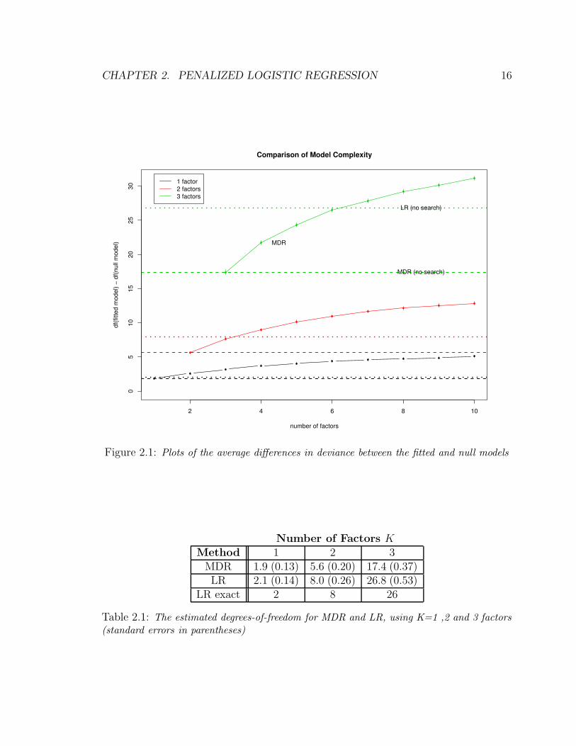
Figure 2.1 captures the results. The black, red, and green solid curves represent the
MDR models with the interaction orders one, two, and three, respectively. The vertical
segments at the junction points are the standard error bars. As the interaction order
increased, the effective degrees of freedom increased as well. In addition, each curve
monotonically increased along with the number of available factors, as the optimal set
of factors was searched over a larger space. The horizontal lines mark the degrees of
freedom from MDR (the lower dotted line) and logistic regression (the upper dotted
line) without searching (we used a fixed set of factors, so that there was no effect due
to searching for an optimal set of factors). These are summarized as well in Table 2.1.
LR exact refers to the asymptotic exact degrees of freedom. For example, an MDR
model with a third-order interaction of three-level factors has an effective dimension
of 17.4 - above half way between the claimed 1 and the 26 of LR.
2.2.2 Conditional logistic regression
Conditional logistic regression (LR) is an essential tool for the analysis of categorical
factors with binary responses. Unlike MDR, LR is able to fit additive and other lower
CHAPTER 2. PENALIZED LOGISTIC REGRESSION 16
2 4 6 8 10
05
1015
2025
30
Comparison of Model Complexity
number of factors
df(fi
tted
mod
el) −
df(n
ull m
odel
) MDR
MDR (no search)
LR (no search)
1 factor2 factors3 factors
Figure 2.1: Plots of the average differences in deviance between the fitted and null models
Number of Factors KMethod 1 2 3
MDR 1.9 (0.13) 5.6 (0.20) 17.4 (0.37)LR 2.1 (0.14) 8.0 (0.26) 26.8 (0.53)
LR exact 2 8 26
Table 2.1: The estimated degrees-of-freedom for MDR and LR, using K=1 ,2 and 3 factors(standard errors in parentheses)

CHAPTER 2. PENALIZED LOGISTIC REGRESSION 17
order effects as well as full-blown interactions. Therefore, LR can yield a more precise
interpretation that distinguishes the presence of additive effects from the presence
of interaction effects. In fact, the users of MDR fit LR models using the factors
selected by MDR precisely for this reason; to simplify the high-order interactions into
its component effects. LR is sometimes criticized due to the difficulties of estimating
a large number of parameters with a relatively small number of samples (Ritchie
et al. 2001); however, we provide a solution to overcome this drawback. Biologists
(Coffey et al. 2004, for example) have shown that LR performs as well as other methods
in cases where it is able to be fit.
2.2.3 FlexTree
Huang et al. (2004) proposed a tree-structured learning method, FlexTree, to identify
the genes related to the cause of complex diseases along with their interactions. It
is a rather complex procedure that aims to build a tree with splits in the form of a
linear combination of multiple factors. Beginning from the root node that contains all
the observations, each node is recursively split into two daughter nodes, through the
following steps:
1. Use backward shaving to select the optimal set of predictors for splitting the
specific node. For the backward shaving, form a decreasing series of candi-
date subsets based on the bootstrapped scores. Then determine the best subset
among the series that yields the largest cross-validated impurity measure.
2. Perform a permutation test to see if the linear relationship between the selected
subset of predictors and the outcome is strong enough. If so, go to the next step.
If not, stop splitting the node.
3. Use the selected subset of predictors to compute the regression coefficients (β)
and the splitting threshold (C) such that a binary split is determined based on

CHAPTER 2. PENALIZED LOGISTIC REGRESSION 18
x′β ≥ C. The optimal scoring method is used for estimating β, and C is chosen
to maximize the resulting Gini index for the node.
Huang et al. (2004) compared FlexTree to other methods such as CART, QUEST,
logic regression, bagging, MART, and random forest; they showed that FlexTree per-
formed better than or as well as these competing methods. Using a very similar
dataset, we compared the performance of our method with that of FlexTree (in Sec-
tion 2.5).
2.3 Penalized Logistic Regression
The generic logistic regression model has the form
logPr(Y = 1|X)
Pr(Y = 0|X)= β0 + XT β,
where X is a vector of predictors (typically dummy variables derived from factors,
in the present setting). Logistic regression coefficients are typically estimated by
maximum-likelihood (McCullagh & Nelder 1989); in fact the deviance (2.1) that we
used in Section 2.2.1 is twice the negative log-likelihood. Here we maximize the log-
likelihood subject to a size constraint on L2 norm of the coefficients (excluding the
intercept) as proposed in Lee & Silvapulle (1988) and Le Cessie & Van Houwelingen
(1992). This amounts to minimizing the following equation:
L(β0, β, λ) = −l(β0, β) +λ
2‖β‖22, (2.2)
where l indicates the binomial log-likelihood, and λ is a positive constant. The coef-
ficients are regularized in the same manner as in ridge regression (Hoerl & Kennard
1970). The importance of the quadratic penalty, particularly in our application, will
CHAPTER 2. PENALIZED LOGISTIC REGRESSION 19
be elaborated in subsequent sections.
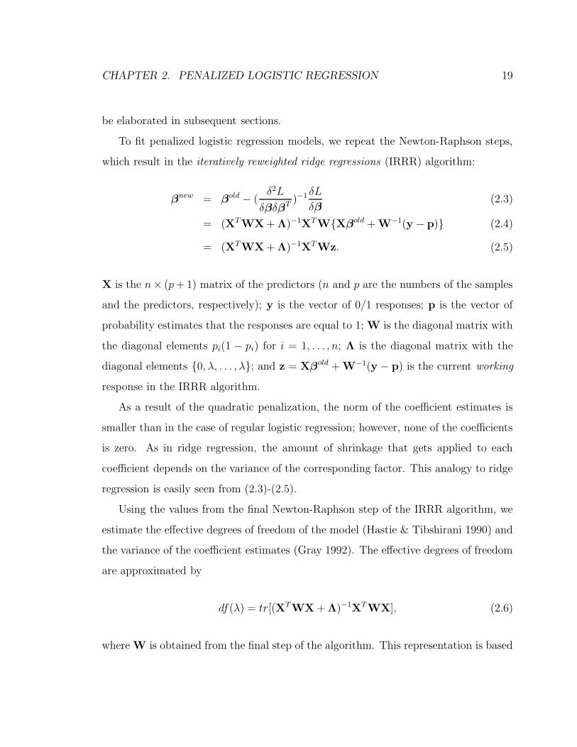
To fit penalized logistic regression models, we repeat the Newton-Raphson steps,
which result in the iteratively reweighted ridge regressions (IRRR) algorithm:
βnew = βold − (δ2L
δβδβT)−1 δL
δβ(2.3)
= (XTWX + Λ)−1XTW{Xβold + W−1(y − p)} (2.4)
= (XTWX + Λ)−1XTWz. (2.5)
X is the n× (p + 1) matrix of the predictors (n and p are the numbers of the samples
and the predictors, respectively); y is the vector of 0/1 responses; p is the vector of
probability estimates that the responses are equal to 1; W is the diagonal matrix with
the diagonal elements pi(1 − pi) for i = 1, . . . , n; Λ is the diagonal matrix with the
diagonal elements {0, λ, . . . , λ}; and z = Xβold + W−1(y − p) is the current working
response in the IRRR algorithm.
As a result of the quadratic penalization, the norm of the coefficient estimates is
smaller than in the case of regular logistic regression; however, none of the coefficients
is zero. As in ridge regression, the amount of shrinkage that gets applied to each
coefficient depends on the variance of the corresponding factor. This analogy to ridge
regression is easily seen from (2.3)-(2.5).
Using the values from the final Newton-Raphson step of the IRRR algorithm, we
estimate the effective degrees of freedom of the model (Hastie & Tibshirani 1990) and
the variance of the coefficient estimates (Gray 1992). The effective degrees of freedom
are approximated by
df(λ) = tr[(XTWX + Λ)−1XTWX], (2.6)
where W is obtained from the final step of the algorithm. This representation is based

CHAPTER 2. PENALIZED LOGISTIC REGRESSION 20
on similar ideas to those described in Section 2.2.1. The variance of the coefficients is
also estimated from the final iteration:
V ar(β) = V ar[(XTWX + Λ)−1XTWz] (2.7)
= (XTWX + Λ)−1V ar[XT (y − p)](XTWX + Λ)−1 (2.8)
= (δ2L
δβδβT)−1I(β)(
δ2L
δβδβT)−1, (2.9)
where I(β) denotes the information in y. This is referred to as a sandwich estimate
(Gray 1992).
We now elaborate on the use of penalized logistic regression specifically as it relates
to our problem.
2.3.1 Advantages of quadratic penalization
Using quadratic regularization with logistic regression has a number of attractive prop-
erties.
1. When we fit interactions between categorical factors, the number of parameters
can grow large. The penalization nevertheless enables us to fit the coefficients
in a stable fashion.
2. We can code factors in a symmetric fashion using dummy variables, without the
usual concern for multicollinearity. (In Section 2.3.4, we introduce a missing
value imputation method taking advantage of this coding scheme.)
3. Zero cells are common in multi-factor contingency tables. These situations are
handled gracefully.
Since quadratic regularization overcomes collinearity amongst the variables, a pe-
nalized logistic regression model can be fit with a large number of factors or high-order

CHAPTER 2. PENALIZED LOGISTIC REGRESSION 21
interaction terms. The sample size does not limit the number of parameters. In Sec-
tion 2.3.2, we illustrate our variable selection strategy; a growing number of variables
in the model is not detrimental to the variable search.
The quadratic penalty makes it possible to code each level of a factor by a dummy
variable, yielding coefficients with direct interpretations. Each coefficient reveals the
significance of a particular level of a factor. This coding method cannot be applied
to regular logistic regression because the dummy variables representing a factor are
perfectly collinear (they sum to one). To overcome this, one of the levels is omitted,
or else the levels of the factors are represented as contrasts.
It turns out that the penalized criterion (2.2) creates the implicit constraint that
the coefficients of the dummy variables representing any discrete factor/interaction of
factors must sum to zero. Consider the model
logPr(Y = 1|D)
Pr(Y = 0|D)= β0 + DT β, (2.10)
where D is a vector of dummy variables that represent the levels of a three-level
categorical factor. As can be seen from (2.10), adding a constant vector to β and
subtracting the same constant from β0 would not change the probability estimate.
However, because our criterion minimizes ‖β‖2, the coefficients are identifiable in such
a way that the elements of β sum to zero. Given a dataset of n observations (di, yi),
we differentiate the objective function (2.2) with respect to the coefficients and obtain:
δL
δβ0
= 0 ⇐⇒n
∑
i=1
(yi − pi) = 0,
δL
δβ= 0 ⇐⇒
n∑
i=1
(yi − pi)di = λβ. (2.11)

CHAPTER 2. PENALIZED LOGISTIC REGRESSION 22
These equations, in turn, imply∑3
j=1 βj = 0. It can easily be shown that similar reduc-
tions hold with higher-order interaction terms as well. Zhu & Hastie (2004) explored
this property of the L2 penalization in (multinomial) penalized logistic regression using
continuous factors.
When a column of X is so unbalanced that it contains no observations at a par-
ticular level (or combination of levels), the corresponding dummy variable is zero for
all n observations. This phenomenon is common in SNP data because one allele of
a locus can easily be prevalent over the other allele on the same locus. The lack of
observations for certain levels of factors occurs even more frequently in high-order
interaction models. We cannot fit a regular logistic regression model with an input
matrix that contains a column of zeros. However, when logistic regression is accompa-
nied by any small amount of quadratic penalization, the coefficient of the zero column
will automatically be zero.
We demonstrate this for a simple two-way interaction term in a model. As in
(2.11),δL
δβ12jk
= 0⇐⇒ λβ12jk = mjk −
1
1 + e−(β0+β1
j +β2
k+β12
jk)njk,
where njk is the number of observations with X1 = j and X2 = k, mjk is the number
among these with Y = 1, and β1j is the coefficient for the jth level of variable 1, etc.
The equivalence implies that if njk = 0, then mjk = 0, and, thus, β12jk = 0 for any
λ > 0. An analogous equality holds at any interaction order.
This equation also illustrates the stability that is imposed, for example, if mjk = 0
while njk > 0. In the unregularized case this would lead to convergence problems, and
coefficients running off to infinity.

CHAPTER 2. PENALIZED LOGISTIC REGRESSION 23
2.3.2 Variable selection
Penalizing the norm of the coefficients results in a smoothing effect for most cases.
However, with an L2 penalization, none of the coefficients is set to zero unless the
distribution of the factors is extremely sparse as illustrated in the previous section.
For prediction accuracy and interpretability, we often prefer using only a subset of the
features in the model, and thus we must design another variable selection tool. We
choose to run a forward selection, followed by a backward deletion.
In each forward step, a factor/interaction of factors is added to the model. A
fixed number of forward steps are repeated. In the following backward steps, a fac-
tor/interaction of factors is deleted, beginning with the final, and thus the largest,
model from the forward steps; the backward deletion continues until only one factor
remains in the active set (the set of variables in the model). The factor to be added or
deleted in each step is selected based on the score defined as deviance+ cp×df, where
cp is complexity parameter. Popular choices are cp = 2 and cp = log(sample size) for
AIC and BIC, respectively.
When adding or deleting variables, we follow the rule of hierarchy: when an inter-
action of multiple factors is in the model, the lower order factors comprising the inter-
action must be also present in the model. However, to allow interaction terms to enter
the model more easily, we modify the convention, such that any factor/interaction of
factors in the active set can form a new interaction with any other single factor, even
when the single factor is not yet in the active set. This relaxed condition of permitting
the interaction terms was suggested in multivariate adaptive regression splines, MARS
(Friedman 1991). To add more flexibility, an option is to provide all possible second-
order interactions as well as main effect terms as candidate factors at the beginning
of the forward steps.
In the backward deletion process, again obeying the hierarchy, no component (of
lower-order) of an interaction term can be dropped before the interaction term. As

CHAPTER 2. PENALIZED LOGISTIC REGRESSION 24
the size of the active set is reduced monotonically, the backward deletion process offers
a series of models, from the most complex model to the simplest one that contains
only one factor. Using the list of corresponding scores, we select the model size that
generated the minimum score.
2.3.3 Choosing the regularization parameter λ
Here we explore the smoothing effect of an L2 penalization, briefly mentioned in Sec-
tion 2.3.2. When building factorial models with interactions, we have to be concerned
with overfitting the data, even with a selected subset of the features. In addition to
the advantages of using quadratic regularization emphasized in Section 2.3.1, it can
be used to smooth a model and thus to control the effective size of the model, through
the effective degrees of freedom (2.6). As heavier regularization is imposed with an
increased λ, the deviance of the fit increases (the fit degrades), but the variance (2.7)-
(2.9) of the coefficients and the effective degrees of freedom (2.6) of the model decrease.
As a result, when the model size is determined based on AIC/BIC, a larger value of λ
tends to choose a model with more variables and allow complex interaction terms to
join the model more easily.
To illustrate these patterns of model selection with varying λ and suggest a method
of choosing an appropriate value, we ran three sets of simulation analyses, for each one
generating data with a different magnitude of interaction effect. For all three cases,
we generated datasets consisting of a binary response and six categorical factors with
three levels. Only the first two of the six predictors affected the response, with the
conditional probabilities of belonging to class 1 as in the tables below. Figure 2.2
displays the log-odds for class 1, for all possible combinations of levels of the first
two factors; the log-odds are additive for the first model, while the next two show
interaction effects.

CHAPTER 2. PENALIZED LOGISTIC REGRESSION 25
Additive Model
P (A) = P (B) = 0.5
BB Bb bb
AA 0.845 0.206 0.206
Aa 0.206 0.012 0.012
aa 0.206 0.012 0.012
Interaction Model I
P (A) = P (B) = 0.5
BB Bb bb
AA 0.145 0.206 0.206
Aa 0.206 0.012 0.012
aa 0.206 0.012 0.012
Interaction Model II
P (A) = P (B) = 0.5
BB Bb bb
AA 0.045 0.206 0.206
Aa 0.206 0.012 0.012
aa 0.206 0.012 0.012
1.0 1.5 2.0 2.5 3.0
−4−3
−2−1
01
Additive Model
1st factor
log−
odds
(Cla
ss 1
)
AA
Aa aaAA
Aa aa
2nd factor = BB2nd factor = Bb, bb
1.0 1.5 2.0 2.5 3.0
−4−3
−2−1
01
Interaction Model I
1st factor
log−
odds
(Cla
ss 1
)
AA
Aa aaAA
Aa aa
2nd factor = BB2nd factor = Bb, bb
1.0 1.5 2.0 2.5 3.0−4
−3−2
−10
1
Interaction Model II
1st factor
log−
odds
(Cla
ss 1
)
AA
Aa aaAA
Aa aa
2nd factor = BB2nd factor = Bb, bb
Figure 2.2: The patterns of log-odds for class 1, for different levels of the first two factors
For each model, we generated 30 datasets of size 100, with balanced class labels.
Then, we applied our procedure with λ = {0.01, 0.5, 1, 2}, for each λ selecting a model
based on BIC. Table 2.2 summarizes how many times A+B (the additive model with
the first two factors) and A ∗ B (the interaction between the first two factors) were
selected. The models that were not counted in the table include A, B, or the ones
with the terms other than A and B. Given that A + B is the true model for the first
set while A∗B is appropriate for the second and the third, ideally we should be fitting
with small values of λ for the additive model but increasing λ as stronger interaction
effects are added.
We can cross-validate to choose the value of λ; for each fold, we obtain a series of
optimal models (based on AIC/BIC) corresponding to the candidate values of λ and

CHAPTER 2. PENALIZED LOGISTIC REGRESSION 26
λ 0.01 0.5 1 2
Additive ModelA + B 28/30 26/30 26/30 22/30A ∗B 0/30 0/30 0/30 5/30
Interaction Model IA + B 16/30 14/30 10/30 6/30A ∗B 11/30 14/30 18/30 23/30
Interaction Model IIA + B 6/30 5/30 3/30 1/30A ∗B 20/30 24/30 26/30 27/30
Table 2.2: The number of times that the additive and the interaction models were selected.A + B is the true model for the first set while A ∗ B is the true model for the second andthe third.
compute the log-likelihoods using the omitted fold. Then we choose the value of λ
that yields the largest average (cross-validated) log-likelihood. We demonstrate this
selection strategy in Section 2.4.
2.3.4 Missing value imputation
The coding method we implemented suggests an easy, but reasonable, method of
imputing any missing values. If there are any samples lacking an observation for a
factor Xj, we then compute the sample proportions of the levels of Xj among the
remaining samples. These proportions, which are the expected values of the dummy
variables, are assigned to the samples with missing cells.
In this scheme, the fact that the dummy variables representing any factor sum to
1 is retained. In addition, our approach offers a smoother imputation than does filling
the missing observations with the level that occurred most frequently in the remaining
data. Through simulations in Section 2.4, we show that this imputation method yields
a reasonable result.

CHAPTER 2. PENALIZED LOGISTIC REGRESSION 27
2.4 Simulation Study
To compare the performance of penalized logistic regression to that of MDR under
various settings, we generated three epistatic models and a heterogeneity model, some
of which are based on the suggestions in Neuman & Rice (1992). Each training dataset
contained 400 samples (200 cases and 200 controls) and 10 factors, only two of which
were significant. Three levels of the two significant factors were distributed so that
the conditional probabilities of being diseased were as in the tables below; the levels
of the remaining eight insignificant factors were in Hardy-Weinberg equilibrium. For
all four examples, the overall proportion of the diseased population was 10%.
Epistatic Model I
P (A) = 0.394, P (B) = 0.340
BB Bb bb
AA 0.7 0.7 0
Aa 0.7 0 0
aa 0 0 0
Epistatic Model III
P (A) = 0.3, P (B) = 0.3
BB Bb bb
AA 0.988 0.5 0.5
Aa 0.5 0.01 0.01
aa 0.5 0.01 0.01
Epistatic Model II
P (A) = 0.450, P (B) = 0.283
BB Bb bb
AA 0 0.4 0.4
Aa 0.4 0 0
aa 0.4 0 0
Heterogeneity Model
P (A) = 0.512, P (B) = 0.303
BB Bb bb
AA 0.415 0.35 0.35
Aa 0.1 0 0
aa 0.1 0 0
Figure 2.3 contains the plots of the log-odds for all the conditional probabilities in
the tables. (Zeros are replaced by 0.001 to compute the log-odds.) As can be seen,
we designed the third epistatic model so that the log-odds are additive (the odds are
multiplicative) in the first two factors; the interaction effect is more obvious in the
first two epistatic models than in the heterogeneity model. Our distinction of the
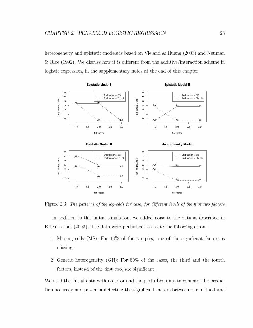
CHAPTER 2. PENALIZED LOGISTIC REGRESSION 28
heterogeneity and epistatic models is based on Vieland & Huang (2003) and Neuman
& Rice (1992). We discuss how it is different from the additive/interaction scheme in
logistic regression, in the supplementary notes at the end of this chapter.
1.0 1.5 2.0 2.5 3.0
−6−2
02
46
Epistatic Model I
1st factor
log−
odds
(Cas
e)
AA Aa
aaAa
2nd factor = BB2nd factor = Bb, bb
1.0 1.5 2.0 2.5 3.0
−6−2
02
46
Epistatic Model II
1st factorlo
g−od
ds(C
ase)
AA
Aa aaAA
Aa aa
2nd factor = BB2nd factor = Bb, bb
1.0 1.5 2.0 2.5 3.0
−6−2
02
46
Epistatic Model III
1st factor
log−
odds
(Cas
e)
AA
Aa aaAA
Aa aa
2nd factor = BB2nd factor = Bb, bb
1.0 1.5 2.0 2.5 3.0
−6−2
02
46
Heterogeneity Model
1st factor
log−
odds
(Cas
e)
AA Aa aaAA
Aa aa
2nd factor = BB2nd factor = Bb, bb
Figure 2.3: The patterns of the log-odds for case, for different levels of the first two factors
In addition to this initial simulation, we added noise to the data as described in
Ritchie et al. (2003). The data were perturbed to create the following errors:
1. Missing cells (MS): For 10% of the samples, one of the significant factors is
missing.
2. Genetic heterogeneity (GH): For 50% of the cases, the third and the fourth
factors, instead of the first two, are significant.
We used the initial data with no error and the perturbed data to compare the predic-
tion accuracy and power in detecting the significant factors between our method and

CHAPTER 2. PENALIZED LOGISTIC REGRESSION 29
MDR.
Under each scenario, we simulated thirty sets of training and test datasets. For
each training set, we selected the regularization parameter λ through cross-validation,
and using the chosen λ, built a model based on the BIC criterion. For each cross-
validation, we provided candidate values of λ in an adaptive way. We first applied a
small value, λ = 10−5, to the whole training dataset and achieved models of different
sizes from the backward deletion. Based on the series of models, we defined a set of
reasonable values for the effective degrees of freedom. Then we computed the values
of λ that would reduce the effective degrees of freedom of the largest model to the
smaller values in the set.
We measured the prediction errors by averaging the thirty test errors. Table 2.3
summarizes the prediction accuracy comparison of penalized logistic regression and
MDR; the standard errors of the error estimates are parenthesized. The table shows
that for both methods, the error rates increase when the data contain errors. The
prediction accuracies are similar between the two methods, although MDR yields
slightly larger error rates in most situations.
Model No error MS GH
Epistatic IStep PLR 0.023(0.001) 0.025(0.001) 0.111(0.002)
MDR 0.023(0.001) 0.029(0.001) 0.131(0.002)
Epistatic IIStep PLR 0.085(0.001) 0.092(0.001) 0.234(0.004)
MDR 0.084(0.001) 0.093(0.002) 0.241(0.004)
Epistatic IIIStep PLR 0.096(0.002) 0.099(0.002) 0.168(0.003)
MDR 0.097(0.002) 0.105(0.002) 0.192(0.005)
HeterogeneityStep PLR 0.144(0.002) 0.146(0.002) 0.304(0.004)
MDR 0.148(0.002) 0.149(0.002) 0.310(0.004)
Table 2.3: The prediction accuracy comparison of step PLR and MDR (the standard errorsare parenthesized)
Table 2.4 contains the numbers counting the cases (out of 30) for which the correct
factors were identified. For step PLR, the number of cases for which the interaction

CHAPTER 2. PENALIZED LOGISTIC REGRESSION 30
terms were also selected is parenthesized; the numbers vary reflecting the magnitude
of interaction effect imposed in these four models as shown in Figure 2.3.
Model No error MS GH
Epistatic IStep PLR 30(27) 30(30) 30(29)
MDR 30 29 30
Epistatic IIStep PLR 30(29) 30(28) 30(25)
MDR 27 29 16
Epistatic IIIStep PLR 30(1) 30(2) 30(2)
MDR 27 29 26
HeterogeneityStep PLR 30(10) 30(10) 30(8)
MDR 23 27 5
Table 2.4: The number of cases (out of 30) for which the correct factors were identified.For step PLR, the number of cases that included the interaction terms is in the parentheses.
For the heterogeneity model, main effects exist for both of the two significant
factors. In addition, as one is stronger than the other, MDR was not successful in
identifying them simultaneously even for the data with no error, as shown in Table 2.4.
In the case of the heterogeneity model or the second epistatic model, MDR suffered
from a decrease in power, especially with GH perturbations. When GH perturbations
were added to the second epistatic model, MDR correctly specified the four factors only
16 out of 30 times, while our method did so in all 3 simulations. These results show
that the penalized logistic regression method is more powerful than MDR, especially
when multiple sets of significant factors exist; in these situations, MDR often identifies
only a subset of the significant factors.
2.5 Real Data Example
2.5.1 Hypertension dataset
We compared our method to Flextree and MDR using the data from the SAPPHIRe
(Stanford Asian Pacific Program for Hypertension and Insulin Resistance) project.

CHAPTER 2. PENALIZED LOGISTIC REGRESSION 31
The goal of the SAPPHIRe project was to detect the genes that predispose individuals
to hypertension. A similar dataset was used in Huang et al. (2004) to show that
the FlexTree method outperforms many competing methods. The dataset contains
the menopausal status and the genotypes on 21 distinct loci of 216 hypotensive and
364 hypertensive Chinese women. The subjects’ family information is also available;
samples belonging to the same family are included in the same cross-validation fold
for all the analyses.
Prediction performance
We applied five-fold cross-validation to estimate the misclassification rates using pe-
nalized logistic regression, FlexTree, and MDR. For penalized logistic regression, a
complexity parameter was chosen for each fold through an internal cross-validation.
MDR used internal cross-validations to select the most significant sets of features; for
each fold, the overall cases/control ratio in the training part was used as the threshold
when we labeled the cells in the tables.
Huang et al. (2004) initially used an unequal loss for the two classes: misclassifying
a hypotension sample was twice as costly as misclassifying a hypertension sample. We
fit penalized logistic regression and FlexTree with an equal as well as an unequal loss.
MDR could only be implemented with an equal loss.
Method (loss) Miscost Sensitivity Specificity
Step PLR (unequal) 141 + 2× 85 = 311 223/364 = 0.613 131/216 = 0.606FlexTree (unequal) 129 + 2× 105 = 339 235/364 = 0.646 111/216 = 0.514Step PLR (equal) 72 + 139 = 211 292/364 = 0.802 77/216 = 0.356FlexTree (equal) 61 + 163 = 224 303/364 = 0.832 53/216 = 0.245
MDR (equal) 92 + 151 = 243 272/364 = 0.747 65/216 = 0.301
Table 2.5: Comparison of prediction performance among different methods
The results are compared in Table 2.5. Penalized logistic regression achieved lower
misclassification cost than FlexTree with either loss function. When an equal loss was

CHAPTER 2. PENALIZED LOGISTIC REGRESSION 32
used, FlexTree and MDR generated highly unbalanced predictions, assigning most
samples to the larger class. Although penalized logistic regression also achieved a low
specificity, it was not so serious as in the other two methods.
0.0 0.2 0.4 0.6 0.8 1.0
0.0
0.2
0.4
0.6
0.8
1.0
ROC curve for PLR: unequal loss
Specificity
Sen
sitiv
ity
PLRFlexTree
0.0 0.2 0.4 0.6 0.8 1.0
0.0
0.2
0.4
0.6
0.8
1.0
ROC curve for PLR: equal loss
Specificity
Sen
sitiv
ity
PLRFlexTreeMDR
Figure 2.4: Receiver operating characteristic (ROC) curves for penalized logistic regressionwith an unequal (left panel) and an equal (right panel) loss function. The red dots representthe values we achieved with the usual threshold 0.5. The green dots correspond to Flextreeand the blue dot corresponds to MDR.
Figure 2.4 shows the receiver operating characteristic (ROC) curves for penalized
logistic regression with an unequal (left panel) and an equal (right panel) loss function.
For both plots, vertical and horizontal axes indicate the sensitivity and the specificity
respectively. Because penalized logistic regression yields the predicted probabilities
of a case, we could compute different sets of sensitivity and specificity by changing
the classification threshold between 0 and 1. The red dots on the curves represent
the values we achieved with the usual threshold 0.5. The green dots corresponding

CHAPTER 2. PENALIZED LOGISTIC REGRESSION 33
to Flextree and the blue dot corresponding to MDR are all located toward the lower
left corner, away from the ROC curves. In other words, penalized logistic regression
would achieve a higher sensitivity (specificity) than other methods if the specificity
(sensitivity) were fixed the same as theirs.
Bootstrap analysis of the feature selection
Applying our forward stepwise procedure to the whole dataset yields a certain set of
significant features as listed in the first column of Table 2.6. However, if the data were
perturbed, a different set of features would be selected. Through a bootstrap analysis
(Efron & Tibshirani 1993), we provide a measure of how likely the features were to be
selected and examine what other factors could have been preferred.
Factors selected from the whole data Frequencymenopause 299/300MLRI2V 73/300
Cyp11B2x1INV ×MLRI2V 3/300KLKQ3E 29/300
KLKQ3E × Cyp11B2x1INV ×MLRI2V 10/300AGT2R1A1166C ×menopause 106/300
Table 2.6: Significant factors selected from the whole dataset (left column) and their fre-quencies in 300 bootstrap runs (right column)
We illustrate the bootstrap analysis using a fixed value of λ. For each of B = 300
bootstrap datasets, we ran a forward stepwise procedure with λ = 0.25, which is a
value that was frequently selected in previous cross-validation. At the end of the
B bootstrap runs, we counted the frequency for every factor/interaction of factors
that has been included in the model at least once. The second column of Table 2.6
contains the counts for the corresponding features; some of them were rarely selected.
Table 2.7 lists the factors/interactions of factors that were selected with relatively high
frequencies.

CHAPTER 2. PENALIZED LOGISTIC REGRESSION 34
Factor Frequency Interaction of factors Frequencymenopause 299/300 menopause× AGT2R1A1166C 106/300MLRI2V 73/300 menopause× ADRB3W1R 48/300
AGT2R1A1166C 35/300 menopause× Cyp11B2x1INV 34/300HUT2SNP5 34/300 menopause× Cyp11B2− 5′aINV 33/300
PTPN1i4INV 34/300 menopause× AV PR2G12E 31/300PPARG12 30/300
Table 2.7: Factors/interactions of factors that were selected in 300 bootstrap runs withrelatively high frequencies
Not all of the commonly selected factors listed in Table 2.7 were included in the
model when we used the whole dataset. It is possible that some factors/interactions of
factors were rarely selected simultaneously because of a strong correlation among them.
To detect such instances, we propose using the co-occurrence matrix (after normalizing
for the individual frequencies) among all the factors/interactions of factors listed in
Table 2.7 as a dissimilarity matrix and applying hierarchical clustering. Then any
group of factors that tends not to appear simultaneously would form tight clusters.
Using the 11 selected features in Table 2.7, we first constructed the 11 × 11 co-
occurrence matrix, so that the (i, j) element was the number of the bootstrap runs in
which the i-th and the j-th features were selected simultaneously. Then we normalized
the matrix by dividing the (i, j) entry by the number of bootstrap runs in which either
the i-th or the j-th feature was selected. That is, denoting the (i, j) entry as Mij, we
divided it by Mii + Mjj −Mij, for every i and j.
As we performed hierarchical clustering with the normalized co-occurrence dis-
tance measure, PTPN1i4INV and MLRI2V were in a strong cluster: they were in
the model simultaneously for only two bootstrap runs. Analogously, AGT2R1A1166C
and menopause×AGT2R1A1166C appeared 35 and 106 times respectively, but only
twice simultaneously. For both clusters, one of the elements was selected in our model
(Table 2.6) while the other was not. Hence, the pairs were presumably used as alter-
natives in different models.
CHAPTER 2. PENALIZED LOGISTIC REGRESSION 35
2.5.2 Bladder cancer dataset
We show a further comparison of different methods with another dataset, which was
used by Hung et al. (2004) for a case-control study of bladder cancer. The dataset
consisted of genotypes on 14 loci and the smoke status of 201 bladder cancer patients
and 214 controls.
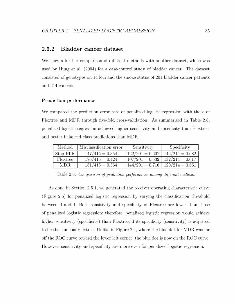
Prediction performance
We compared the prediction error rate of penalized logistic regression with those of
Flextree and MDR through five-fold cross-validation. As summarized in Table 2.8,
penalized logistic regression achieved higher sensitivity and specificity than Flextree,
and better balanced class predictions than MDR.
Method Misclassification error Sensitivity Specificity
Step PLR 147/415 = 0.354 122/201 = 0.607 146/214 = 0.682Flextree 176/415 = 0.424 107/201 = 0.532 132/214 = 0.617MDR 151/415 = 0.364 144/201 = 0.716 120/214 = 0.561
Table 2.8: Comparison of prediction performance among different methods
As done in Section 2.5.1, we generated the receiver operating characteristic curve
(Figure 2.5) for penalized logistic regression by varying the classification threshold
between 0 and 1. Both sensitivity and specificity of Flextree are lower than those
of penalized logistic regression; therefore, penalized logistic regression would achieve
higher sensitivity (specificity) than Flextree, if its specificity (sensitivity) is adjusted
to be the same as Flextree. Unlike in Figure 2.4, where the blue dot for MDR was far
off the ROC curve toward the lower left corner, the blue dot is now on the ROC curve.
However, sensitivity and specificity are more even for penalized logistic regression.
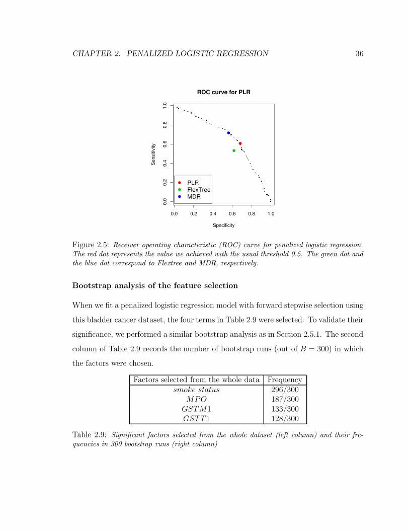
CHAPTER 2. PENALIZED LOGISTIC REGRESSION 36
0.0 0.2 0.4 0.6 0.8 1.0
0.0
0.2
0.4
0.6
0.8
1.0
ROC curve for PLR
Specificity
Sen
sitiv
ity
PLRFlexTreeMDR
Figure 2.5: Receiver operating characteristic (ROC) curve for penalized logistic regression.The red dot represents the value we achieved with the usual threshold 0.5. The green dot andthe blue dot correspond to Flextree and MDR, respectively.
Bootstrap analysis of the feature selection
When we fit a penalized logistic regression model with forward stepwise selection using
this bladder cancer dataset, the four terms in Table 2.9 were selected. To validate their
significance, we performed a similar bootstrap analysis as in Section 2.5.1. The second
column of Table 2.9 records the number of bootstrap runs (out of B = 300) in which
the factors were chosen.
Factors selected from the whole data Frequencysmoke status 296/300
MPO 187/300GSTM1 133/300GSTT1 128/300
Table 2.9: Significant factors selected from the whole dataset (left column) and their fre-quencies in 300 bootstrap runs (right column)

CHAPTER 2. PENALIZED LOGISTIC REGRESSION 37
The factors/interactions of factors that were frequently selected through the boot-
strap runs are listed in Table 2.10. The factors in Table 2.9 form the subset with the
highest ranks among the ones listed in Table 2.10, providing evidence of reliability.
The latter half of Table 2.10 shows that even the interaction terms with the largest
counts were not as frequent as other common main effect terms. When we applied
MDR, the second order interaction term MPO × smoke status was often selected;
however, according to the bootstrap results, logistic regression method can explain
their effect in a simpler, additive model. In addition, MDR was not able to identify
other potentially important features.
Factor Frequency Interaction of factors Frequencysmoke status 296/300 MPO × smoke status 38/300
MPO 187/300 GSTT1×NAT2 34/300GSTM1 133/300 GMSTM1×MnSOD 26/300GSTT1 128/300 GSTT1×XRCC1 24/300NAT2 88/300
MnSOD 67/300
Table 2.10: Factors/interactions of factors that were selected in 300 bootstrap runs withrelatively high frequencies
We also used the co-occurrence matrix of the factors in Table 2.10 as a dissimilarity
measure and applied hierarchical clustering. One of the tightest clusters was the pair
of GSTM1 and NAT2 : they were in the model 133 and 88 times respectively, but
coincided only 33 times, implying that NAT2 was often used to replace GSTM1.
These results from the bootstrap analysis are consistent with the findings in Hung
et al. (2004) in several ways. The factors with high frequencies (the first column of
Table 2.10) are among the ones that were shown to be significantly increasing the risk
of bladder cancer, through conventional analyses reported in Hung et al. (2004). Hung
et al. also incorporated some known facts about the functional similarities of the genes
and improved the estimates of the odds ratio. From this hierarchical modeling, MPO,
GSTM1, and MnSOD achieved high odds ratios with improved accuracy. In addition,

CHAPTER 2. PENALIZED LOGISTIC REGRESSION 38
their analysis of gene-environment interaction showed that although smoking status
itself was a significant factor, none of its interaction with other genes was strikingly
strong. Similarly, as can be seen from Table 2.10, our bootstrap runs did not detect
any critical interaction effect.
2.6 Summary
We have proposed using logistic regression with a penalization on the size of the L2
norm of the coefficients. The penalty was imposed not only for the usual smoothing
effect but also for convenient and sometimes necessary features that the quadratic
penalization accompanied. In regular logistic regression models, a small sample size
prohibits high-order interaction terms, and variables with constant zero entries are
often not allowed. Because these situations are common in modeling gene-gene in-
teractions, logistic regression is limited in its applications. However, the quadratic
penalization scheme yields a stable fit, even with a large number of parameters, and
automatically assigns zero to the coefficients of zero columns.
We modified the hierarchy rule of the forward stepwise procedure to allow the
interaction terms to enter the model more easily. One strategy was to accept an
interaction term as a candidate if either component was already in the model. If a
strong interaction effect with negligible main effects is suspected, more flexible rules,
such as accepting an interaction term even with no main effect terms, should be
applied. However, the forward stepwise procedure selects variables in a greedy manner.
A less greedy selection through L1 regularization will allow the terms to enter the
model more smoothly. For example, we can use the group variable selection methods
proposed in Yuan & Lin (2006), by forming a group for every set of dummy variables
representing a single factor or an interaction of factors. We study these methods
further in Chapter 4.

CHAPTER 2. PENALIZED LOGISTIC REGRESSION 39
Logistic regression yields a reasonable prediction accuracy and identification of
significant factors along with their interaction structures. We have shown that adding
a quadratic penalization is a simple but powerful remedy that makes it possible to use
logistic regression in building gene-gene interaction models.
The forward stepwise procedure with L2 penalized logistic regression has been
implemented in the contributed R package stepPlr available from CRAN.
Supplementary notes: Two-Locus Modeling
Many researchers have suggested methods to categorize two-locus models for genetic
diseases and to mathematically formulate the corresponding probabilities of influ-
encing the disease status. The two-locus models are often divided into two classes:
heterogeneity models for which a certain genotype causes the disease independently
of the genotype on the other locus, and epistatis models for which the two genotypes
are dependent. To represent the two distinct classes, the concept of penetrance is
often used. Penetrance is a genetic term meaning the proportion of individuals with
a disease-causing gene that actually show the symptoms of the disease.
Let A and B denote potential disease-causing genotypes on two different loci, and
use the following notation to formulate different genetic models:
fA = P (Have disease|A),
fB = P (Have disease|B), and
fA,B = P (Have disease|A, B).
That is, fA, fB, and fA,B denote the penetrance, or the conditional probability of
resulting in the disease, for the individuals carrying the genotypes A, B, and both A
and B, respectively.

CHAPTER 2. PENALIZED LOGISTIC REGRESSION 40
Vieland & Huang (2003) defined heterogeneity between two loci to be the relation-
ship with the following fundamental heterogeneity equation:
fA,B = fA + fB − (fA × fB), (2.12)
which is directly derived from the following more obvious representation of the inde-
pendent effect of a pair of genotypes:
1− fA,B = (1− fA)× (1− fB).
They referred to any other two-locus relationship for which (2.12) does not hold as
epistatic. Neuman & Rice (1992) distinguished the heterogeneity models likewise.
Risch (1990) also characterized multiplicative and additive two-locus models; the dis-
ease penetrance for carriers of both genotypes A and B was multiplicative or additive
in the penetrance scores for single genotypes A and B. Risch considered the additive
model to be a reasonable approximation of a heterogeneity model.
As we demonstrated in Section 2.3.3 and Section 2.4, logistic regression identifies
the relationship among the active genes as either additive or having an interaction;
however, this distinction is not equivalent to that of heterogeneity and the epistatic
relationship described above. For example, epistatic model III in Section 2.4 has a
probability distribution such that the conditional probabilities of disease are additive
in log-odds; we expect an additive model when applying logistic regression. Although
in genetics, heterogeneity models are often characterized by no interaction among loci
in affecting the disease, the factors are not necessarily conceived to be additive in
logistic regression. However, in the example illustrated in Section 2.4, the interaction
effect in the heterogeneity model was not as critical as in other epistatic models, and
logistic regression found an additive model in more than 50% of the repeats.

Chapter 3
L1 Regularization Path Algorithm
for Generalized Linear Models
In this chapter, we introduce a path-following algorithm for L1 regularized generalized
linear models. The L1 regularization procedure is useful especially because it, in
effect, selects variables according to the amount of penalization on the L1 norm of the
coefficients, in a manner less greedy than forward selection/backward deletion. The
GLM path algorithm efficiently computes solutions along the entire regularization
path using the predictor-corrector method of convex-optimization. Selecting the step
length of the regularization parameter is critical in controlling the overall accuracy of
the paths; we suggest intuitive and flexible strategies for choosing appropriate values.
We demonstrate the implementation with several simulated and real datasets.
3.1 Background
GLM models a random variable Y that follows a distribution in the exponential fam-
ily using a linear combination of the predictors, x′β, where x and β denote vectors
of the predictors and the coefficients, respectively. The random and the systematic
41

CHAPTER 3. L1 REGULARIZATION PATH ALGORITHM 42
components may be linked through a non-linear function; therefore, we estimate the
coefficient β by solving a set of non-linear equations that satisfy the maximum likeli-
hood criterion.
β = argmaxβ
L(y; β), (3.1)
where L denotes the likelihood function with respect to the given data {(xi, yi) : i =
1, . . . , n}.
When the number of predictors p exceeds the number of observations n, or when
insignificant predictors are present, we can impose a penalization on the L1 norm
of the coefficients for an automatic variable selection effect. Analogous to Lasso
(Tibshirani 1996) that added a penalty term to the squared error loss criterion, we
modify criterion (3.1) with a regularization:
β(λ) = argminβ{− log L(y; β) + λ‖β‖1}, (3.2)
where λ > 0 is the regularization parameter. Logistic regression with L1 penalization
has been introduced and applied by other researchers, for example in Shevade &
Keerthi (2003).
We introduce an algorithm that implements the predictor-corrector method to
determine the entire path of the coefficient estimates as λ varies, i.e., to find {β(λ) :
0 < λ < ∞}. Starting from λ = ∞, our algorithm computes a series of solution sets,
each time estimating the coefficients with a smaller λ based on the previous estimate.
Each round of optimization consists of three steps: determining the step size in λ,
predicting the corresponding change in the coefficients, and correcting the error in the
previous prediction.
A traditional approach to variable selection is the forward selection/backward dele-
tion method that adds/deletes variables in a greedy manner. L1 regularization as in

CHAPTER 3. L1 REGULARIZATION PATH ALGORITHM 43
(3.2) can be viewed as a smoother and “more democratic” version of forward stepwise
selection. The GLM path algorithm is not only less greedy than forward stepwise,
but also provides models throughout the entire range of complexity, whereas forward
stepwise often stops augmenting the model before reaching the most complex stage
possible.
Efron et al. (2004) suggested an efficient algorithm to determine the exact piece-
wise linear coefficient paths for Lasso; see Osborne et al. (2000) for a closely related
approach. The algorithm called Lars is also used for forward stagewise and least an-
gle regression paths with slight modifications. Another example of a path-following
procedure is SVM path (Hastie et al. 2004). They presented a method of drawing the
entire regularization path for support vector machine simultaneously.
Unlike Lars or SVM paths, the GLM paths are not piecewise linear. We must select
particular values of λ at which the coefficients are computed exactly; the granularity
controls the overall accuracy of the paths. When the coefficients are computed on a
fine grid of values for λ, the nonlinearity of the paths is more visible. Because it is
interesting to know the locations along the paths at which the set of nonzero coefficients
changes, we propose a way to compute the exact coefficients at those values of λ.
Rosset (2004) suggested a general path-following algorithm that can be applied
to any loss and penalty function with reasonable bounds on the domains and the
derivatives. This algorithm computes the coefficient paths in two steps: changing λ
and updating the coefficient estimates through a Newton iteration. Zhao & Yu (2004)
proposed Boosted Lasso that approximates the L1 regularization path with respect
to any convex loss function by allowing backward steps to forward stagewise fitting;
whenever a step in forward stagewise fitting deviated from that of Lasso, Boosted
Lasso would correct the step with a backward move. When this strategy is used
with minus log-likelihood (of a distribution in the exponential family) loss function,
it will approximate the L1 regularized GLM path. As discussed by Zhao and Yu, the

CHAPTER 3. L1 REGULARIZATION PATH ALGORITHM 44
step sizes along the path are distributed such that Zhao and Yu’s method finds the
exact solutions at uniformly spaced values of ‖β‖1, while Rosset’s method computes
solutions at uniformly spaced λ. Our method is more flexible and efficient than these
two approaches; we estimate the largest λ that will change the current active set
of variables and solve for the new set of solutions at the estimated λ. Hence, the
step lengths are not uniform for any single parameter but depend on the data; at
the same time, we ensure that the solutions are exact at the locations where the
active set changes. We demonstrate the accuracy and the efficiency of our strategy in
Section 3.3.2.
Other researchers have implemented algorithms for L1 regularized logistic regres-
sion for diverse applications. For example, Genkin et al. (2004) proposed an algorithm
for L1 regularized logistic regression (for text categorization) in a Bayesian context,
in which the parameter of the prior distribution was their regularization parameter.
They chose the parameter based on the norm of the feature vectors or through cross-
validation, performing a separate optimization for each potential value. Our method
of using the solutions for a certain λ as the starting point for the next, smaller λ offers
the critical advantage of reducing the number of computations.
In the following sections, we describe and support our approach in more detail
with examples and justifications. We present the details of the GLM path algorithm
in Section 3.2. In Section 3.3, our methods are illustrated with simulated and real
datasets, including a microarray dataset consisting of over 7000 genes. We illustrate
an extension of our path-following method to the Cox proportional hazards model
in Section 3.4. We conclude with a summary and other possible extensions of our
research in Section 3.5.
CHAPTER 3. L1 REGULARIZATION PATH ALGORITHM 45
3.2 GLM Path Algorithm
In this section, we describe the details of the GLM path algorithm. We compute
the exact solution coefficients at particular values λ, and connect the coefficients in a
piecewise linear manner for solutions corresponding to other values of λ.
3.2.1 Problem setup
Let {(xi, yi) : xi ∈ Rp, yi ∈ R, i = 1, . . . , n} be n pairs of p factors and a response.
Y follows a distribution in the exponential family with mean µ = E(Y ) and variance
V = V ar(Y ). Depending on its distribution, the domain of yi could be a subset of R.
GLM models the random component Y by equating its mean µ with the systematic
component η through a link function g :
η = g(µ) = β0 + x′β.
The likelihood of Y is expressed as follows (McCullagh & Nelder 1989):
L(y; θ, φ) = exp{(yθ − b(θ))/a(φ) + c(y, φ)}.
a(·), b(·), and c(·) are functions that vary according to the distributions. Assuming
that the dispersion parameter φ is known, we are interested in finding the maximum
likelihood solution for the natural parameter θ, and thus (β0, β′)′, with a penalization
on the size of the L1 norm of the coefficients (‖β‖1). Therefore, our criterion with a
fixed λ is reduced to finding β = (β0, β′)′, which minimizes the following:
l(β, λ) = −n
∑
i=1
{yiθ(β)i − b(θ(β)i)}+ λ‖β‖1. (3.3)

CHAPTER 3. L1 REGULARIZATION PATH ALGORITHM 46
Assuming that none of the components of β is zero and differentiating l(β, λ) with
respect to β, we define a function H :
H(β, λ) =δl
δβ= −X′W(y− µ)
δη
δµ+ λSgn
(
0
β
)
, (3.4)
where X is an n by (p + 1) matrix including the column of 1′s, W is a diagonal
matrix with n diagonal elements V −1i ( δµ
δη)2i , and (y−µ) δη
δµis a vector with n elements
(yi − µi)(δηδµ
)i. Although we have assumed that none of the elements of β is zero,
the set of nonzero components of β changes with λ, and H(β, λ) must be redefined
accordingly.
Our goal is to compute the entire solution path for the coefficients β, with λ
varying from ∞ to 0. We achieve this by drawing the uniquely determined curve
H(β, λ) = 0 in (p + 2) dimensional space (β ∈ Rp+1 and λ ∈ R+). Because l(β, λ)
is a convex function of β, there exists a β(λ) that attains the unique minimum value
for each λ ∈ R+. In fact, a unique continuous and differentiable function β(λ), such
that H(β(λ), λ) = 0 exists within each open range of λ that yields a certain active
set of variables; the existence of such mappings (λ → β(λ)) can be shown using the
implicit function theorem (Munkres 1991). We find the mapping β(λ) sequentially
with decreasing λ.
3.2.2 Predictor - Corrector algorithm
The predictor-corrector algorithm is one of the fundamental strategies for implement-
ing numerical continuation (introduced and applied in various publications, for ex-
ample, in Allgower & Georg (1990) and Garcia & Zangwill (1981)). Numerical con-
tinuation has long been used in mathematics to identify the set of solutions to non-
linear equations that are traced through a 1-dimensional parameter. Among many
approaches, the predictor-corrector method explicitly finds a series of solutions by

CHAPTER 3. L1 REGULARIZATION PATH ALGORITHM 47
using the initial conditions (solutions at one extreme value of the parameter) and con-
tinuing to find the adjacent solutions based on the current solutions. We elaborate on
how the predictor-corrector method is used to trace the curve H(β, λ) = 0 through λ
in our problem setting.
The following lemma provides the initialization of the coefficient paths:
Lemma 3.2.1. When λ exceeds a certain threshold, the intercept is the only nonzero
coefficient: β0 = g(y) and
H((β0, 0, . . . , 0)′, λ) = 0 for λ > maxj∈{1,...,p}
|x′jW(y − y1)g′(y)|. (3.5)
Proof. The Karush-Kuhn-Tucker (KKT) optimality conditions for minimizing (3.3)
imply
∣
∣
∣x′
jW(y − µ)δη
δµ
∣
∣
∣< λ =⇒ βj = 0 for j = 1, . . . , p. (3.6)
When βj = 0 for all j = 1, . . . , p, the KKT conditions again imply
1′W(y − µ)δη
δµ= 0,
which, in turn, yields µ = y1 = g−1(β0)1.
As λ is decreased further, other variables join the active set, beginning with the
variable j0 = argmaxj |x′j(y− y1)|. Reducing λ, we alternate between a predictor and
a corrector step; the steps of the k-th iteration are as follows:
1. Step length: determine the decrement in λ. Given λk, we approximate the next
largest λ, at which the active set changes, namely λk+1.
2. Predictor step: linearly approximate the corresponding change in β with the
decrease in λ; call it βk+
.

CHAPTER 3. L1 REGULARIZATION PATH ALGORITHM 48
3. Corrector step: find the exact solution of β that pairs with λk+1 (i.e., β(λk+1)),
using βk+
as the starting value; call it βk+1
.
4. Active set: test to see if the current active set must be modified; if so, repeat
the corrector step with the updated active set.
Predictor step
In the k-th predictor step, β(λk+1) is approximated by
βk+
= βk
+ (λk+1 − λk)δβ
δλ(3.7)
= βk− (λk+1 − λk)(X
′AWkXA)−1Sgn
0
βk
. (3.8)
Wk and XA denote the current weight matrix and the columns of X for the factors
in the current active set, respectively. β in the above equations are composed only
of current nonzero coefficients. This linearization is equivalent to making a quadratic
approximation of the log-likelihood and extending the current solution βk
by taking
a weighted Lasso step (as in LARS).
Define f(λ) = H(β(λ), λ); in the domain that yields the current active set, f(λ)
is zero for all λ. By differentiating f with respect to λ, we obtain
f ′(λ) =δH
δλ+
δH
δβ
δβ
δλ= 0,
from which we compute δβ/δλ.
Corrector step
In the following corrector step, we use βk+
as the initial value to find the β that
minimizes l(β, λk+1), as defined in (3.3) (i.e., that solves H(β, λk+1) = 0 for β).

CHAPTER 3. L1 REGULARIZATION PATH ALGORITHM 49
Any (convex) optimization method that applies to the minimization of a differentiable
objective function with linear constraints may be implemented. The previous predictor
step has provided a warm start; because βk+
is usually close to the exact solution βk+1
,
the cost of solving for the exact solution is low. The corrector steps not only find the
exact solutions at a given λ but also yield the directions of β for the subsequent
predictor steps.
Active set
The active set A begins from the intercept as in Lemma 3.2.1; after each corrector
step, we check to see if A should have been augmented. The following procedure for
checking is justified and used by Rosset & Zhu (2004) and Rosset (2004):
∣
∣
∣x′
jW(y− µ)δη
δµ
∣
∣
∣> λ for any j ∈ Ac =⇒ A← A∪ {j}.
We repeat the corrector step with the modified active set until the active set is not
augmented further. We then remove the variables with zero coefficients from the active
set. That is,
|βj| = 0 for any j ∈ A =⇒ A← A− {j}.
Step length
Two natural choices for the step length ∆k = λk − λk+1 are:
• ∆k = ∆, fixed for every k, or
• a fixed change L in L1 arc-length, achieved by setting ∆k = L/‖δβ/δλ‖1.
As we decrease the step size, the exact solutions are computed on a finer grid of λ
values, and the coefficient path becomes more accurate.

CHAPTER 3. L1 REGULARIZATION PATH ALGORITHM 50
We propose a more efficient and useful strategy:
• select the smallest ∆k that will change the active set of variables.
We give an intuitive explanation of how we achieve this, by drawing on analogies
with the Lars algorithm (Efron et al. 2004). At the end of the k-th iteration, the
corrector step can be characterized as finding a weighted Lasso solution that satisfies
−X′AWk(y − µ) δη
δµ+ λkSgn
(
0β
)
= 0. This weighted Lasso also produces the direction
for the next predictor step. If the weights Wk were fixed, the weighted Lars algorithm
would be able to compute the exact step length to the next active-set change point. We
use this step length, even though in practice the weights change as the path progresses.
Lemma 3.2.2. Let µ be the estimates of y from a corrector step, and denote the
corresponding weighted correlations as
c = X′W(y − µ)δη
δµ.
The absolute correlations of the factors in A (except for the intercept) are λ, while the
values are smaller than λ for the factors in Ac.
Proof. The Karush-Kuhn-Tucker (KKT) optimality conditions for minimizing (3.3)
imply
βj 6= 0 =⇒∣
∣
∣x′
jW(y − µ)δη
δµ
∣
∣
∣= λ.
This condition, combined with (3.5) and (3.6), proves the argument.

CHAPTER 3. L1 REGULARIZATION PATH ALGORITHM 51
The next predictor step extends β as in (3.8), and, thus, the current correlations
change. Denoting the vector of changes in correlation for a unit decrease in λ as a,
c(h) = c− ha
= c− hX′WXA(X′AWXA)−1Sgn
(
0
β
)
,
where h > 0 is a given decrease in λ. For the factors in A, the values of a are those of
Sgn(
0β
)
. To find the h with which any factor in Ac yields the same absolute correlation
as the ones in A, we solve the following equations:
|cj(h)| = |cj − haj| = λ− h for any j ∈ Ac.
The equations suggest an estimate of the step length in λ as
h = min+
j∈Ac{λ− cj
1− aj,λ + cj
1 + aj}.
In addition, to check if any variable in the active set reaches 0 before λ decreases by
h, we solve the equations
βj(h) = βj + h(X′AWXA)−1Sgn
(
0
β
)
= 0 for any j ∈ A. (3.9)
If 0 < h < h for any j ∈ A, we expect that the corresponding variable will be
eliminated from the active set before any other variable joins it; therefore, h rather
than h is used as the next step length.
Letting the coefficient paths be piecewise linear with the knots placed where the
active set changes is a reasonable simplification of the truth based on our experience
(using both simulated and real datasets). If the smallest step length that modifies the
active set were to be larger than the value we have estimated, the active set remains

CHAPTER 3. L1 REGULARIZATION PATH ALGORITHM 52
the same, even after the corrector step. If the true step length were smaller than
expected, and, thus, we missed the entering point of a new active variable by far, we
would repeat a corrector step with an increased λ. (We estimate the increase in a
manner analogous to (3.9).) Therefore, our path algorithm almost precisely detects
the values of λ at which the active set changes, in the sense that we compute the
exact coefficients at least once before their absolute values grow larger than δ (a small
fixed quantity). δ can be set to be any small constant; one can evaluate how small it
is using the standard error estimates for the coefficients from the bootstrap analysis,
which is illustrated later in Section 3.3.2.
We can easily show that in the case of Gaussian distribution with the identity link,
the piecewise linear paths are exact. Because µ = Xβ, and Vi = V ar(yi) is constant
for i = 1, . . . , n, H(β, λ) simplifies to −X′(y − µ) + λSgn(
0β
)
. The step lengths are
computed with no error; in addition, since the predictor steps yield the exact coefficient
values, corrector steps are not necessary. In fact, the paths are identical to those of
Lasso.
3.2.3 Degrees of freedom
We use the size of the active set as a measure of the degrees of freedom, which changes,
not necessarily monotonically, along the solution paths. That is,
df(λ) = |A(λ)|, (3.10)
where |A(λ)| denotes the size of the active set corresponding to λ. We present a
heuristic justification for using (3.10), based on the results developed in Zou & Hastie
(2004).
One can show that the estimates of β at the end of a corrector step solve a weighted

CHAPTER 3. L1 REGULARIZATION PATH ALGORITHM 53
Lasso problem,
minβ
(z−Xβ)TW(z−Xβ) + λ||β||1, (3.11)
where the working response vector is defined as
z = η + (y − µ)δη
δµ.
The solution to (3.11) would be an appropriate fit for a linear model
z = Xβ + ε where ε ∼ (0,W−1). (3.12)
This covariance is correct at the true values of η and µ, and can be defended asymp-
totically if appropriate assumptions are made. In fact, when λ = 0, and assuming ε
has a Gaussian distribution, (3.12) leads directly to the standard asymptotic formulas
and Gaussianity for the maximum-likelihood estimates in the exponential family. 1
Under these heuristics, we apply the Stein’s Lemma (Stein 1981) to the transformed
response (W1/2z) so that its errors are homoskedastic. We refer readers to Zou &
Hastie (2004) for the details of the application of the lemma. Their Theorem 2 shows
df(λ) = E|A(λ)| in the case of Lasso; we derive the degrees of freedom of L1 regularized
GLM in a similar manner. Simulations show that (3.10) approximates the degrees of
freedom reasonably closely, although we omit the details here.
3.2.4 Adding a quadratic penalty
When some columns of X are strongly correlated, the coefficient estimates are highly
unstable; the solution might not be unique if some columns are redundant. Osborne
et al. (2000) provided a necessary and sufficient condition for the existence of a unique
1This assumption is clearly not true for Bernoulli responses; however, if y represents groupedbinomial proportions, then under the correct asymptotic assumptions ε is Gaussian.

CHAPTER 3. L1 REGULARIZATION PATH ALGORITHM 54
solution. To overcome these situations, we propose adding a quadratic penalty term
to the criterion, following the elastic net proposal of Zou & Hastie (2005). That is, we
compute the solution paths that satisfy the following:
β(λ1) = argminβ
{− log L(y; β) + λ1‖β‖1 +λ2
2‖β‖22}, (3.13)
where λ1 ∈ (0,∞), and λ2 is a fixed, small, positive constant. As a result, strong corre-
lations among the features do not affect the stability of the fit. When the correlations
are not strong, the effect of the quadratic penalty with a small λ2 is negligible.
Assuming that all the elements of β are nonzero, if X does not have a full column
rank, δH(β, λ)/δβ = X′WX is singular, where H is defined as in (3.4). By adding a
quadratic penalty term, as in (3.13), we redefine H :
H(β, λ1, λ2) = −X′W(y − µ)δη
δµ+ λ1Sgn
(
0
β
)
+ λ2
0
β
. (3.14)
Accordingly, the following δH/δβ is non-singular, in general, with any λ2 > 0 :
δH
δβ= X′WX + λ2
0 0′
0 I
.
Therefore, when λ2 is fixed at a constant, and λ1 varies in an open set, such that the
current active set remains the same, a unique, continuous, and differentiable function
β(λ1) satisfies H(β(λ1), λ1, λ2) = 0. This connection between the non-singularity and
existence of a unique, continuous and differentiable coefficient path is based on the
implicit function theorem (Munkres 1991).
In the case of logistic regression, adding an L2 penalty term is also helpful as it
elegantly handles the separable data. Without the L2 penalization, and if the data are
separable by the predictors, ‖β‖1 grows to infinity as λ1 approaches zero. Rosset et al.

CHAPTER 3. L1 REGULARIZATION PATH ALGORITHM 55
(2004) showed that the normalized coefficients β/‖β‖1 converge to the L1 margin-
maximizing separating hyperplane as λ1 decreases to zero. In such cases, the fitted
probabilities approach 0/1, and, thus, the maximum likelihood solutions are undefined.
However, by restricting ‖β‖2 with any small amount of quadratic penalization, we let
the coefficients converge to the L2 penalized logistic regression solutions instead of
infinity as λ1 approaches zero.
Zou & Hastie (2005) proposed elastic net regression, which added an L2 norm
penalty term to the criterion for Lasso. Zou and Hastie adjusted the values of both λ1
and λ2 so that variable selection and grouping effects were achieved simultaneously.
For our purpose of handling inputs with strong correlations, we fixed λ2 at a very
small number, while changing the value of λ1 for different amounts of regularization.
3.3 Data Analysis
In this section, we demonstrate our algorithm through a simulation and two real
datasets: South African heart disease data and leukemia cancer gene expression data.
Our examples focus on binary data, hence the logistic regression GLM.
3.3.1 Simulated data example
We simulated a dataset of 100 observations with 5 variables and a binary response.
Figure 3.1 shows two sets of coefficient paths with respect to λ, with a different selec-
tion of step sizes. In the left panel, the exact solutions were computed at the values of
λ where the active set changed, and the solutions were connected in a piecewise linear
manner. The right panel shows the paths with exact solutions on a much finer grid
of λ values; we controlled the arc length to be less than 0.1 between any two adjacent
values of λ. We observe the true curvature of the paths. The left panel is a reasonable
approximation of the right, especially because the active set is correctly specified at

CHAPTER 3. L1 REGULARIZATION PATH ALGORITHM 56
any value of λ.
**
**
**
*
*
0 5 10 15
−1.5
−1.0
−0.5
0.0
0.5
1.0
1.5
lambda
Sta
ndar
dize
d co
effic
ient
s
******
*
*
****
**
*
*
****
**
*
*
*******
*
Coefficient path
x4
x3
x5
x2
x1
5 4 3 2 1
************************
******
******
*******
******
******
**********
**********
0 5 10 15
−1.5
−1.0
−0.5
0.0
0.5
1.0
1.5
lambda
Sta
ndar
dize
d co
effic
ient
s
*****************************
*********
**********
**********
**********
*******
***************************************************************************
***************************************************************************
***************************************************
*****************
*******
Coefficient path
x4
x3
x5
x2
x1
5 4 3 2 1
Figure 3.1: Comparison of the paths with different selection of step sizes. (left panel) Theexact solutions were computed at the values of λ where the active set changed. (right panel)We controlled the arc length to be less than 0.1 between any two adjacent values of λ.
3.3.2 South African heart disease data
This dataset consists of 9 different features of 462 samples as well as the responses
indicating the presence of heart disease. The dataset has also been used in Hastie
et al. (2001) with a detailed description of the data. Using the disease/non-disease
response variable, we can fit a logistic regression path.
Selecting the step length
The first plot of Figure 3.2 shows the exact set of paths; the coefficients were precisely
computed at 300 different values of λ ranging from 81.9 to 0, with the constraint that
every arc length be less than 0.01. The L1 norm of the coefficients forms the x-axis,
and the vertical breaks indicate where the active set is modified. Comparing this plot
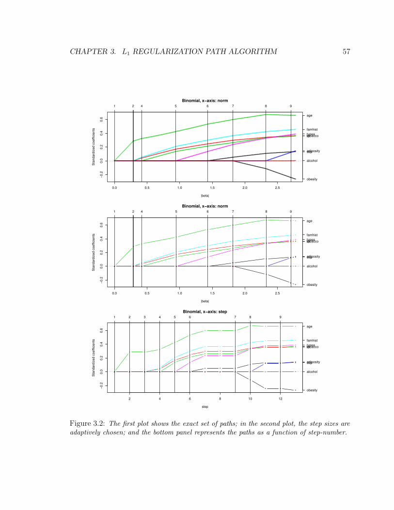
CHAPTER 3. L1 REGULARIZATION PATH ALGORITHM 57
******************************************************************************************************************************************************************************************************************
**************************************************************************
*************************
0.0 0.5 1.0 1.5 2.0 2.5
−0.2
0.0
0.2
0.4
0.6
|beta|
Sta
ndar
dize
d co
effic
ient
s
******************************************************
***************************
********************************
*********************************************
********************************************************
***********************************************************************************************
**********************************************************************
***************************
*****************************************
*************************************************
**************************************************
************************************************************************
**************************************************************************************************************************************************************************************************************************************************************************************
***********************
********
*************************************************
**********************
************************
********************************
*************************************
********************************************
******************************************************************
***********************************
******************************************************************************************************************************
**************************
***************************
*******************************
************************************
************************************************
***************
*********************************************************************************************************************************************************************************************************************************************************************************************************************
*****************************************************************************************************************************************************************************************************************************************************************************************************************************
********
********
************
********************************
*********************************
********************************
*********************************
******************************************
***********************************************
******************************************************
Binomial, x−axis: norm
obesity
alcohol
sbpadiposity
ldltobaccotypeafamhist
age
1 2 4 5 6 7 8 9
* ** * * ****
* ** *
0.0 0.5 1.0 1.5 2.0 2.5
−0.2
0.0
0.2
0.4
0.6
|beta|
Sta
ndar
dize
d co
effic
ient
s
* ***
**
**** ** *
* ** *
*
****
* ** *
* ** * * * *** *
** *
* ***
*
****
* ** *
* ** * *
*
***
*** *
* ** * * * ***
*
** *
* ** * * * *** * ** **
***
*
****
* ** *
Binomial, x−axis: norm
obesity
alcohol
sbpadiposity
ldltobaccotypeafamhist
age
1 2 4 5 6 7 8 9
* * * * * ** * *
* * * *
2 4 6 8 10 12
−0.2
0.0
0.2
0.4
0.6
step
Sta
ndar
dize
d co
effic
ient
s
* * **
**
* * ** * * *
* * * *
*
** * *
* * * *
* * * * * * * * * *
* * *
* * **
*
** * *
* * * *
* * * * *
*
* * *
** * *
* * * * * * * * *
*
* * *
* * * * * * * * * * * * **
* **
*
** * *
* * * *
Binomial, x−axis: step
obesity
alcohol
sbpadiposity
ldltobaccotypeafamhist
age
1 2 3 4 5 6 7 8 9
Figure 3.2: The first plot shows the exact set of paths; in the second plot, the step sizes areadaptively chosen; and the bottom panel represents the paths as a function of step-number.

CHAPTER 3. L1 REGULARIZATION PATH ALGORITHM 58
to the second panel, which we achieved in 13 steps rather than 300, we find that the
two are almost identical. Our strategy to find the λ values at which the active set
changes resulted in an estimate of the values with reasonable accuracy. In addition,
the exact paths are curvy but are almost indistinguishable from the piecewise linear
version, justifying our simplification scheme. For both plots, the right-most solutions
corresponding to λ = 0 are the maximum likelihood estimates.
The bottom panel of Figure 3.2 illustrates the paths with respect to the steps. Two
extra steps were needed between the knots at which the sixth and the seventh variable
joined the active set. However, the step lengths in λ are tiny in this region; since the
first approximation of λ that would change the active set was larger than the true
value by only a small amount, λ decreased again by extremely small amounts. For
most other steps, the subsequent λ′s that would modify the active set were accurately
estimated on their first attempts.
We have proposed three different strategies for selecting the step sizes in λ in
Section 3.2.2:
1. Fixing the step size ∆: ∆k = ∆
2. Fixing the arc length L: ∆k = L/‖δβ/δλ‖1
3. Estimating where the active set changes
To verify that Method 3 yields more accurate paths with a smaller number of steps
and, thus, a smaller number of computations, we present the following comparison.
For the three methods, we counted the number of steps taken and computed the
corresponding sum of squared errors in β,∑200
m=1 ‖β(m) − β(m)‖2. β(m) and β(m) denote
the coefficient estimates at the m-th (out of 200 evenly spaced grid values in ‖β‖1)
grid along the path, from the path generated using a certain step length computation
method and the exact path, respectively.

CHAPTER 3. L1 REGULARIZATION PATH ALGORITHM 59
Method 1 Method 2 Method 3∆ num. steps error L num. steps error num. steps error8 12 2.56e-1 0.23 11 1.01e-1 13 7.11e-41 83 2.04e-1 0.1 26 7.78e-2
0.3 274 6.75e-3 0.02 142 2.28e-20.15 547 7.16e-5 0.01 300 4.25e-5
Table 3.1: Comparison of different strategies for setting the step sizes
As shown in the first row of Table 3.1, the first two strategies of selecting the step
lengths, with a comparable number of steps, achieved much lower accuracy than the
third. Furthermore, the first two methods needed a few hundred steps to yield the same
accuracy that the third method achieved in only 13 steps. Thus, Method 3 provides
accuracy and efficiency in addition to the information about where the junction points
are located.
Bootstrap analysis of the coefficients
Given the series of solution sets with a varying size of the active set, we select an
appropriate value of λ and, thus, a set of coefficients. We may then validate the
chosen coefficient estimates through a bootstrap analysis (Efron & Tibshirani 1993).
We illustrate the validation procedure, choosing the λ that yields the smallest BIC
(Bayesian information criteria). For each of the B = 1000 bootstrap samples, we
fit a logistic regression path and selected λ that minimized the BIC score, thereby
generating a bootstrap distribution of each coefficient estimate. Table 3.2 summarizes
the coefficient estimates computed from the whole data, the mean and the standard
error of the estimates computed from the B bootstrap samples, and the percentage of
the bootstrap coefficients at zero. For the variables with zero coefficients (adiposity,
obesity, and alcohol), over 60% of the bootstrap estimates were zero.
Figure 3.3 shows the bootstrap distributions of the standardized coefficients. Under
the assumption that the original data were randomly sampled from the population,
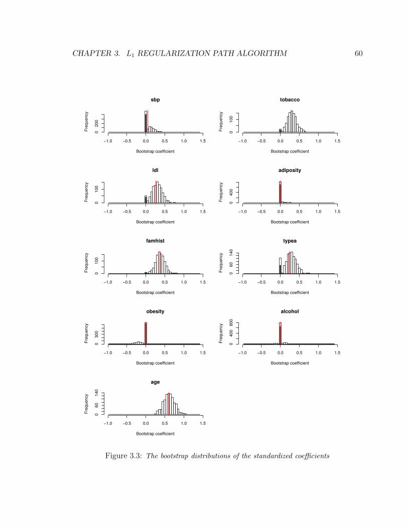
CHAPTER 3. L1 REGULARIZATION PATH ALGORITHM 60
sbp
Bootstrap coefficient
Freq
uenc
y
−1.0 −0.5 0.0 0.5 1.0 1.5
020
0tobacco
Bootstrap coefficient
Freq
uenc
y
−1.0 −0.5 0.0 0.5 1.0 1.5
010
0
ldl
Bootstrap coefficient
Freq
uenc
y
−1.0 −0.5 0.0 0.5 1.0 1.5
010
0
adiposity
Bootstrap coefficientFr
eque
ncy
−1.0 −0.5 0.0 0.5 1.0 1.5
040
0
famhist
Bootstrap coefficient
Freq
uenc
y
−1.0 −0.5 0.0 0.5 1.0 1.5
010
0
typea
Bootstrap coefficient
Freq
uenc
y
−1.0 −0.5 0.0 0.5 1.0 1.5
060
140
obesity
Bootstrap coefficient
Freq
uenc
y
−1.0 −0.5 0.0 0.5 1.0 1.5
030
0
alcohol
Bootstrap coefficient
Freq
uenc
y
−1.0 −0.5 0.0 0.5 1.0 1.5
040
080
0
age
Bootstrap coefficient
Freq
uenc
y
−1.0 −0.5 0.0 0.5 1.0 1.5
060
140
Figure 3.3: The bootstrap distributions of the standardized coefficients

CHAPTER 3. L1 REGULARIZATION PATH ALGORITHM 61
Feature β Mean(βb) SE(βb) Num. zero/Bsbp 0.0521 0.0857 0.1048 0.397
tobacco 0.2988 0.3018 0.1269 0.015ldl 0.2636 0.2925 0.1381 0.040
adiposity 0 0.0367 0.1192 0.700famhist 0.3633 0.3755 0.1218 0.006typea 0.2363 0.2672 0.1420 0.054
obesity 0 -0.0875 0.1510 0.633alcohol 0 0.0078 0.0676 0.646
age 0.5997 0.6109 0.1478 0.000
Table 3.2: The coefficient estimates computed from the whole data, the mean and the stan-dard error of the estimates computed from the B bootstrap samples, and the percentage ofthe bootstrap coefficients at zero
the histograms display the distributions of the coefficient estimates chosen by BIC
criterion. As marked by the red vertical bars, coefficient estimates from the whole
data that are nonzero fall near the center of the bootstrap distributions. For the
predictors whose coefficients are zero, the histograms peak at zero. The thick vertical
bars show the frequencies of zero coefficients.
3.3.3 Leukemia cancer gene expression data
The GLM path algorithm is suitable for data consisting of far more variables than the
samples (so-called p � n scenarios) because it successfully selects up to n variables
along the regularization path regardless of the number of input variables. We demon-
strate this use of our algorithm through a logistic regression applied to the leukemia
cancer gene expression dataset by Golub et al. (1999). The dataset contains the train-
ing and the test samples of sizes 38 and 34, respectively. For each sample, 7129 gene
expression measurements and a label indicating the cancer type (AML: acute myeloid
leukemia or ALL: acute lymphoblastic leukemia) are available.
The first panel of Figure 3.4 shows the coefficient paths we achieved using the
training data; the size of the active set cannot exceed the sample size at any segment

CHAPTER 3. L1 REGULARIZATION PATH ALGORITHM 62
of the paths (This fact is proved in Rosset et al. (2004)). The vertical line marks
the chosen level of regularization (based on cross-validation), where 23 variables had
nonzero coefficients. The second panel of Figure 3.4 illustrates the patterns of ten-fold
cross-validation and test errors. As indicated by the vertical line, we selected λ where
the cross-validation error achieved the minimum.
Table 3.3 shows the errors and the number of variables used in the prediction. We
also compared the performance to other methods that used the same dataset in their
literature. With a cross-validation error of 1/38 and a test error of 2/34, L1 penalized
logistic regression is comparable to or more accurate than other competing methods for
analysis of this microarray dataset. Although we did not perform any pre-processing
to filter from the original 7129 genes, the automatic gene selection reduced the number
of effective genes to 23.
Method CV error Test error Num. genes
L1 PLR 1/38 2/34 23L2 PLR (UR): (Zhu & Hastie 2004) 2/38 3/34 16L2 PLR (RFE): (Zhu & Hastie 2004) 2/38 1/34 26
SVM (UR): (Zhu & Hastie 2004) 2/38 3/34 22SVM (RFE): (Zhu & Hastie 2004) 2/38 1/34 31
NSC classification: (Tibshirani et al. 2002) 1/38 2/34 21
Table 3.3: Comparison of the prediction errors and the number of variables used in theprediction for different methods
3.4 L1 Regularized Cox Proportional Hazards Mod-
els
The path-following method that we applied to the L1 regularized GLM may also be
used to generate other nonlinear regularization paths. We illustrate an analogous
implementation of the predictor-corrector method for drawing the L1 regularization
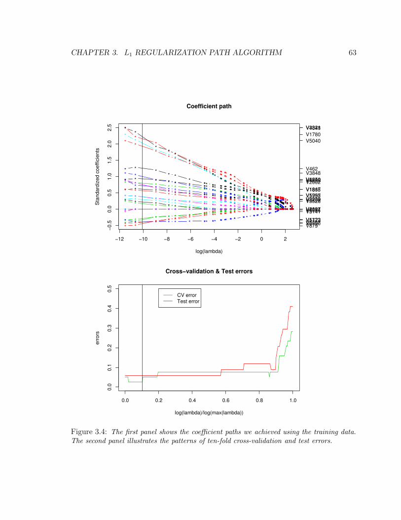
CHAPTER 3. L1 REGULARIZATION PATH ALGORITHM 63
***************************
*******************************************
*****
−12 −10 −8 −6 −4 −2 0 2
−0.5
0.0
0.5
1.0
1.5
2.0
2.5
log(lambda)
Sta
ndar
dize
d co
effic
ient
s
***************************************************************************
***************************************************************************
***************************************************************************
************************************
****************
*****************
***
*
**
***************************************************************************
****************************************
***********************************
***************************************************************************
****************************************
***********************************
*************************************************************************** ***************************************************************************
*************************************************************************** ***************************************************************************
*********
*******************************
************
******************
**
**
*
***************************************************************************
************************************
***************************************
*************************************************************************** ***************************************************************************
*****************************
*************************************
****
**
*
**
**************
**************************************
******************
***
**
***************************************************************************
***************************************************************************
***************************************************************************
*************************************************************************** ************************************
***************************************
***************************************************************************
Coefficient path
V879V6990V5767V5773V1122
V3141V6056V4197V2021
V3526V3209V2239V1797V5955V1835V1847V2002V4665V6540V1250V3848V462
V5040V1780V4848V3321
0.0 0.2 0.4 0.6 0.8 1.0
0.0
0.1
0.2
0.3
0.4
0.5
Cross−validation & Test errors
log(lambda)/log(max(lambda))
erro
rs
CV errorTest error
Figure 3.4: The first panel shows the coefficient paths we achieved using the training data.The second panel illustrates the patterns of ten-fold cross-validation and test errors.

CHAPTER 3. L1 REGULARIZATION PATH ALGORITHM 64
path for the Cox proportional hazards model (Cox 1972). Tibshirani (1997) proposed
fitting the Cox model with a penalty on the size of the L1 norm of the coefficients.
This shrinkage method computes the coefficients with a criterion similar to (3.2):
β(λ) = argminβ{− log L(y; β) + λ‖β‖1}, (3.15)
where L denotes the partial likelihood. We formulate the entire coefficient paths
{β(λ) : 0 < λ < ∞} through the predictor-corrector scheme. As a result of L1
penalization, the solutions are sparse; thus, the active set changes along with λ.
3.4.1 Method
Let {(xi, yi, δi) : xi ∈ Rp, yi ∈ R+, δi ∈ {0, 1}, i = 1, . . . , n} be n triples of p factors,
a response indicating the survival time, and a binary variable, δi = 1 for complete
(died) observations, while δi = 0 for right-censored patients. Based on the criterion
(3.15), we find the coefficients that minimize the following objective function for each
λ :
l(β, λ) = −n
∑
i=1
δiβ′xi +
n∑
i=1
δi log(∑
j∈Ri
eβ′xj) + λ‖β‖1,
where Ri is the set of indices for the patients at risk at time yi-0. To compute the
coefficients, we solve H(β, λ) = 0 for β, where H is defined as follows using only the
current nonzero components of β :
H(β, λ) =δl
δβ= −
n∑
i=1
δixi +n
∑
i=1
δi
∑
j∈Ri
wijxj + λSgn(β),

CHAPTER 3. L1 REGULARIZATION PATH ALGORITHM 65
where wij = eβ′xj/∑
j∈Rieβ′xj . Its derivative is denoted as
δH
δβ=
δ2l
δβδβ ′=
n∑
i=1
δi{∑
j∈Ri
xjx′jwij − (
∑
j∈Ri
xjwij)(∑
j∈Ri
x′jwij)}
= X′AX,
where A = δl2
δηδη′with η = Xβ.
If βj = 0 for j = 1, . . . , p, then wij = 1/|Ri| for i = 1, . . . , n and j = 1, . . . , p, and
δl
δβ= −
n∑
i=1
δi(xi −1
|Ri|
∑
j∈Ri
xj).
βj = 0 for all j if λ > maxj∈{1,...,p} |δl/δβj|. As λ is decreased further, an iterative
procedure begins; variables enter the active set, beginning with j0 = argmaxj|δl/δβj|.
The four steps of an iteration are as follows:
1. Predictor step
In the k-th predictor step, β(λk+1) is approximated as in (3.7), with
δβ
δλ= −
(δH
δβ
)−1 δH
δλ= −(X′
AAXA)−1Sgn(β).
XA contains the columns of X for the current active variables.
2. Corrector step
In the k-th corrector step, we compute the exact solution β(λk+1) using the
approximation from the previous predictor step as the initial value.
3. Active set
Denoting the correlation between the factors and the current residual as c,
c =
n∑
i=1
δixi −n
∑
i=1
δi
∑
j∈Ri
wijxj. (3.16)

CHAPTER 3. L1 REGULARIZATION PATH ALGORITHM 66
After each corrector step, if |cl| > λ for any l ∈ Ac, we augment the active set
by adding xl. Corrector steps are repeated until the active set is not augmented
further. If βl = 0 for any l ∈ A, we eliminate xl from the active set.
4. Step length
If λ = 0, the algorithm stops. If λ > 0, we approximate the smallest decrement
in λ with which the active set will be modified. As λ is decreased by h, the
approximated change in the current correlation (3.16) is as follows:
c(h) = c− hX′AXA(XAAXA)−1Sgn(β). (3.17)
Based on (3.17), we approximate the next largest λ at which the active set will
be augmented/reduced.
3.4.2 Real data example
We demonstrate the L1 regularization path algorithm for the Cox model using the
heart transplant survival data introduced in Crowley & Hu (1977). The dataset con-
sists of 172 samples with the following four features, as well as their survival time and
censor information:
• age: age − 48 years
• year: year of acceptance, in years after 11/1/1967
• surgery: prior bypass surgery, 1, if yes
• transplant: received transplant, 1, if yes
In the top panel of Figure 3.5, the coefficients were computed at fine grids of λ,
whereas in the bottom panel, the solutions were computed only when the active set

CHAPTER 3. L1 REGULARIZATION PATH ALGORITHM 67
* *** * * * * * * * * * *** * * * * * * * * * * * * * * * * * * * * * * * * * * * * * * * * * * * * ** * * * * * * * * * * * * * * * * * * * * * * * * * * * * * * * * * * * * * * * * * * * **
0.0 0.2 0.4 0.6 0.8
−0.2
0.0
0.1
0.2
|beta|
Sta
ndar
dize
d co
effic
ient
s* *** * * * * * * * * * *** * * * * * * * * * * * * * * * * * * * * * * * * * * * * * * * * * * * * ** * * * * * * * * * * * * * * * * * * * * * * * * * * * * * * * * * * * * * * * * * * * **
* *** * * * * * * * * * *** * * * * * * * * * * * * * * * * * * * * * * * * * * * * * * * * * * * * ** * * * * * * * * * * * * * * * * * * * * * * * * * * * * * * * * * * * * * * * * * * * **
* *** * * * * * * * * * *** * * * * * * * * * * * * * * * * * * * * * * * * * * * * * * * * * * * * ** * * * * * * * * * * * * * * * * * * * * * * * * * * * * * * * * * * * * * * * * * * * **
Coefficient path
yearsurgery
transplant
age
0 2 3
* ** **
*
*
0.0 0.2 0.4 0.6 0.8
−0.2
0.0
0.1
0.2
|beta|
Sta
ndar
dize
d co
effic
ient
s
* **
**
*
*
* ****
*
*
* ** ** *
*
Coefficient path
yearsurgery
transplant
age
0 2 3
Figure 3.5: In the top panel, the coefficients were computed at fine grids of λ, whereas in thebottom panel, the solutions were computed only when the active set was expected to change.
was expected to change. Similar to the GLM path examples, the exact coefficient
paths shown on the top plot are almost piecewise linear; it is difficult to distinguish
the two versions generated by different step sizes in λ.
3.5 Summary
In this chapter, we have introduced a path-following algorithm to fit generalized linear
models with L1 regularization. As applied to regression (Tibshirani 1996, Tibshirani
1997) and classification methods (Genkin et al. 2004, Shevade & Keerthi 2003, Zhu
et al. 2003), penalizing the size of the L1 norm of the coefficients is useful because it
accompanies variable selection. This strategy has provided us with a much smoother
feature selection mechanism than the forward stepwise process.
Although the regularization parameter (λ in our case) influences the prediction
performance in the aforementioned models considerably, determining the parameter
CHAPTER 3. L1 REGULARIZATION PATH ALGORITHM 68
can be troublesome or demand heavy computation. The GLM path algorithm facili-
tates model selection by implementing the predictor-corrector method and finding the
entire regularization path sequentially, thereby avoiding independent optimization at
different values of λ. Even with large intervals in λ, the predictor steps provide the
subsequent corrector steps with reasonable estimates (starting values); therefore, the
intervals can be wide without increasing the computations by a large number, as long
as the paths can be assumed to be approximately linear within the intervals.
In Section 3.3.2, we proposed three different methods to form such intervals and
emphasized the efficiency and accuracy of the strategy of finding the transition points.
One may suggest a more naive approach of pre-selecting certain values of λ and gen-
erating the coefficient paths by connecting the solutions to those grids. However, as
shown in the comparison of the methods summarized in Table 3.1, such a strategy will
generate paths that are either inaccurate or demand computations.
We can extend the use of the predictor-corrector scheme by generalizing the loss
+ penalty function to any convex and almost differentiable functions. For example,
we can find the entire regularization path for the Cox proportional hazards model
with L1 penalization, as described in Section 3.4. Rosset & Zhu (2004) illustrated
sufficient conditions for the regularized solution paths to be piecewise linear. Just
as the solution paths for Gaussian distribution were computed with no error through
the predictor-corrector method, so any other piecewise linear solution paths can be
computed exactly by applying the same strategy.
The path-following algorithms for GLM and Cox proportional hazards model have
been implemented in the contributed R package glmpath available from CRAN.

Chapter 4
Regularization Path Algorithms for
Detecting Gene Interactions
In this chapter, we consider several regularization path algorithms with grouped vari-
able selection for modeling gene-interactions. When fitting with categorical factors,
including the genotype measurements, we often define a set of dummy variables that
represent a single factor/interaction of factors. Yuan & Lin (2006) proposed the group-
Lars and the group-Lasso methods through which these groups of indicators can be
selected simultaneously. Here we introduce another version of group-Lars. In addi-
tion, we propose a path-following algorithm for the group-Lasso method applied to
generalized linear models. We then use all these path algorithms, which select the
grouped variables in a smooth way, to identify gene-interactions affecting disease sta-
tus in an example. We further compare their performance to that of L2 penalized
logistic regression with forward stepwise variable selection discussed in Chapter 2.
69

CHAPTER 4. GROUPED VARIABLE SELECTION 70
4.1 Background
We propose using regularization path algorithms with grouped variable selection for
fitting a binary classification model with genotype data and for identifying signif-
icant interaction effects among the genes. We implement the group-Lars and the
group-Lasso methods introduced in Yuan & Lin (2006), and we also introduce a dif-
ferent version of the group-Lars method. To fit the nonlinear regularization path
for group-Lasso, we develop an algorithm based on the predictor-corrector scheme as
in Chapter 3. Our group-Lasso algorithm can use any loss function in the family
of generalized linear models. We regard this strategy of using path algorithms as a
compromise between our two earlier studies, described next.
In Chapter 2, we proposed using forward stepwise logistic regression to fit gene-
interaction models. The forward stepwise procedure is a traditional variable selection
mechanism; we made a set of dummy variables for each factor/interaction of factors
and added/deleted a group at a time. In many studies dealing with gene-interactions,
logistic regression has been criticized for its limited applicability: a small sample size
prohibits high-order interaction terms, and a sparse distribution of the genotypes (for
a factor/interaction of factors) is not tolerated as it results in zero column inputs.
However, by modifying logistic regression with a slight penalty on the L2 norm of
the coefficients, we could fit a stable gene-interaction model. Although the forward
stepwise method is a greedy approach, we showed that it successfully selected signif-
icant terms and achieved a reasonable prediction accuracy when combined with the
L2 penalized logistic regression.
A smoother way to select the features that has been explored extensively in many
regression/classification settings is to incorporate an L1 norm constraint. Tibshirani
(1996) first introduced Lasso, a regression method that minimizes the sum of squared
error loss subject to an L1 norm constraint on the coefficients. Various applications

CHAPTER 4. GROUPED VARIABLE SELECTION 71
of the L1 norm penalty can be found for example in Genkin et al. (2004), Tibshirani
(1997), or Zhu et al. (2003). Efron et al. (2004) proposed the Lars algorithm, a slight
modification of which gave a fast way to fit the entire regularization path for Lasso.
Motivated by this algorithm, we proposed a path-following algorithm for L1 regular-
ized generalized linear models, which generates piecewise-smooth paths (Chapter 3).
Rosset (2004), and Zhao & Yu (2004) also developed algorithms that serve the same
purpose. While these algorithms are limited to selecting a single term at a time, the
group-Lars and the group-Lasso methods mentioned earlier select features as a group,
among the predefined sets of variables.
To fit gene-interaction models with the data consisting of genotype measurements
and a binary response, we first construct sets of indicators representing all the available
factors and all possible two-way interactions. We then provide these grouped variables
to the path algorithms. Although we expected an improvement in terms of correct
feature selection and prediction accuracy over our L2 penalized stepwise logistic re-
gression approach, which selects variables in a greedy manner, this was not always
the case. We showed that these smoother methods perform no better than stepwise
logistic regression, mainly because they tend to select large groups of variables too
easily.
In the following sections, we illustrate several regularization schemes for grouped
variable selection in detail and compare their performance with that of stepwise logistic
regression with L2 penalization. In Section 4.2, we describe the group-Lars and the
group-Lasso methods; in addition, we propose a modified group-Lars algorithm and
a path-following procedure for group-Lasso. We present detailed simulation results in
Section 4.3 and a real data example in Section 4.4. We conclude with a summary and
further thoughts in Section 4.5.

CHAPTER 4. GROUPED VARIABLE SELECTION 72
4.2 Regularization Methods for Grouped Variable
Selection
In this section, we review the group-Lars and the group-Lasso methods proposed by
Yuan & Lin (2006) and propose another version of group-Lars. We call these two
group-Lars methods Type I and Type II, respectively. We describe a path-following
algorithm for group-Lasso, which uses the predictor-corrector convex optimization
scheme as in Chapter 3.
4.2.1 Group-Lars: Type I
Efron et al. (2004) proposed least angle regression (LARS) as a procedure that is
closely related to Lasso and that provides a fast way to fit the entire regularization
path for Lasso. At the beginning of the Lars algorithm, a predictor that is most
strongly correlated with the response enters the model. The coefficient of the chosen
predictor grows in the direction of the sign of its correlation. The single coefficient
grows until another predictor achieves the same absolute correlation with the current
residuals. At this point, both coefficients start moving in the least squares direction
of the two predictors; this is also the direction that keeps their correlations with the
current residuals equal. At each subsequent step, a new variable is added to the model
and the path extends in a piecewise-linear fashion. The path is completed either when
the size of the active set reaches the sample size, or when all the variables are active
and have attained the ordinary least squares fit. As the Lars path proceeds, all the
active variables carry the same, and the largest, amount of correlation with the current
residuals. Yuan & Lin’s group-Lars algorithm operates in a similar way: a group is
included in the model if and only if the average squared correlation of the variables in
the group is the largest, and thus, the same as other active groups.

CHAPTER 4. GROUPED VARIABLE SELECTION 73
The group-Lars algorithm proceeds as follows:
1. The algorithm begins by computing the average squared correlation of the ele-
ments in each group, with the response.
2. The group of variables with the largest average squared correlation enters the
model, and the coefficients of all its components move in the least squares direc-
tion.
3. The first segment of the path extends linearly until the average squared corre-
lation of another group meets that of the active group.
4. Once the second group joins, the coefficients of all the variables in the two groups
again start moving in their least squares direction.
5. Analogously, a new group enters the model at each step until all the groups are
added, and all the individual predictors are orthogonal to the residuals, with
zero correlations.
Once a group has entered the active set, its average squared correlation with the
residuals stays the same as other active groups because all the individual correlations
(their absolute values) decrease proportionally to their current sizes. We can compute
how long a segment of a path extends until the next group joins the active set by
solving a set of quadratic equations. If the total number of the predictors would
exceed the sample size with the addition of the next group, then the algorithm must
stop without adding the new candidate group.
4.2.2 Group-Lars: Type II
The group-Lars Type I algorithm controls groups of different sizes by tracing their
average squared correlations; however, squaring the individual correlations sometimes

CHAPTER 4. GROUPED VARIABLE SELECTION 74
makes a few strongest predictors in the group dominate the average score. We propose
another variant of the Lars algorithm for group variable selection that lessens such
effect; our algorithm traces the average absolute correlation for each group instead
of the average squared correlation. The most important difference in effect is that
our strategy requires more components of a group to be strongly correlated with
the residuals (in a relative sense, when compared to the previous Type I algorithm).
Therefore, our algorithm tracking the average absolute correlation is more robust
against false positives of selecting large groups when only a few of the elements are
strongly correlated with the residuals.
The Type II algorithm is identical to the enumerated description of the Type I
algorithm in Section 4.2.1, except that the average squared correlation is replaced
by the average absolute correlation. Here we illustrate the algorithm using the same
mathematical notation as in Efron et al. (2004):
• The given data are {(X,y) : X ∈ Rn×p,y ∈ Rn}. n is the sample size. Denote
the columns of X as xj, j = 1, . . . , p, and assume that each column has been
centered to have mean zero. The p variables have been partitioned into K
disjoint groups G1, . . . , GK.
• The initial residuals are r = y− y1, where y denotes the mean of the vector y.
• For each group, compute the average absolute correlation of the variables with
the residuals. Select the group with the largest average absolute correlation:
k∗ = argmaxk∈{1,...,K}
∑
j∈Gk
|x′jr|/|Gk|,
where |Gk| denotes the group size for Gk. The corresponding group forms the
active set: A = Gk∗ and Ac = {1, . . . , p} \Gk∗.
• Repeat the following while |A| ≤ n and∑
j∈A |x′jr| > 0.

CHAPTER 4. GROUPED VARIABLE SELECTION 75
1. Let uA be the unit vector toward the least squares direction of {xj : j ∈ A}.
2. If Ac = ∅, then find how much to extend uA so that all the average abso-
lute correlations for the active groups decrease to zero. That is, solve the
following equation for γ > 0 for any Gk ⊂ A :
∑
j∈Gk
|x′j(r− γuA)|/|Gk| = 0.
Denote the solution as γ.
3. If Ac 6= ∅, then for every group in Ac, find how much to extend uA so that
the average absolute correlation for the group is the same as those in A.
That is, for all Gl ⊂ Ac, solve the following equation for γ > 0 :
∑
j∈Gl
|x′j(r− γuA)|/|Gl| =
∑
j∈Gk
|x′j(r− γuA)|/|Gk|,
where Gk is any group in A. Among the solution γ ′s, choose the smallest
positive value, and call it γ. Letting Gl∗ be the corresponding group index,
enlarge the active set: A = A ∪Gl∗, and Ac = Ac \Gl∗.
4. Compute the residuals: r = r− γuA.
For each run of the above enumerated steps, the unit vector uA for a linear segment
of the path can be expressed in a simple form. Denote the sub-matrix of X for the
active variables as XA, and define the following:
cA = X′Ar, GA = X′
AXA, AA = (c′AG−1A cA)−1/2. (4.1)
Then uA = AAXAG−1A cA is the unit vector in the direction of µA = XAG−1
A X′Ay, the
full least squares fit using the current active set. It can be easily shown that in every

CHAPTER 4. GROUPED VARIABLE SELECTION 76
run, γ ∈ [0, 1/AA], and it equals the upper bound 1/AA when there is no additional
variable to enter the model as in Step 2.
The following lemma ensures that the average absolute correlations stay identical
across all the groups in the active set as the path proceeds, given that the average
absolute correlation of each group had been the same as the rest (the ones who joined
A earlier) at its entry.
Lemma 4.2.1. Let µ = Xβ be the fitted values with some coefficient estimates β.
Let r = y − µ and c = X′r denote the residuals and their correlations with the
predictors, respectively. If β extends in the least squares direction for r, then the
entries of |c| decrease at the rate proportional to their current sizes. That is, denoting
the correlations at α ∈ [0, 1] as c(α),
|c(α)| = (1− α)|c|.
Proof. Denoting the least squares direction as µ,
µ = X(X′X)−1X′r.
Thus,
|c(α)| = |X′(r− αµ)| = |X′r− αX′r| = (1− α)|c|.
If we apply the group-Lars methods to over-represented groups of dummy variables
(dummy variables summing up to 1), the paths may not be unique or suffer from a
singularity issue. To avoid such problems, we add a slight L2 norm penalty to the
sum of squared error loss and formulate the Lars algorithms the same way. This
modification simply amounts to extending the LARS-EN algorithm, a variant of the

CHAPTER 4. GROUPED VARIABLE SELECTION 77
Lars algorithm proposed by Zou & Hastie (2005), to a version that performs grouped
variable selection.
4.2.3 Group-Lasso
Criterion
Yuan & Lin (2006) introduced the group-Lasso method, which finds the coefficients
that minimize the following criterion:
L(β; λ) =1
2‖y −Xβ‖22 + λ
K∑
k=1
√
|Gk|‖βk‖2, (4.2)
where λ is a positive regularization parameter, and βk denotes the elements of β
corresponding to the group Gk. We can replace the loss function (sum of squared error
loss above) with that of generalized linear models. The criterion (4.2) is now written
in this general form:
L(β; λ) = −l(y; β) + λ
K∑
k=1
√
|Gk|‖βk‖2, (4.3)
where y is the response vector that follows a distribution in exponential family, and l
is the corresponding log-likelihood. Meier et al. (2006) studied the properties of this
criterion for the binomial case and proposed an algorithm.
When the response y is Gaussian, the criterion of minimizing (4.2) may be written

CHAPTER 4. GROUPED VARIABLE SELECTION 78
in this equivalent form:
Minimize t
subject to ‖y −Xβ‖2 ≤ t,
‖βk‖2 ≤ ak for k = 1, . . . , K,K
∑
k=1
√
|Gk| ak ≤ s,
where β, a, and t are the variables, and s is a fixed value that replaces λ in (4.2).
This formulation suggests that the minimization can be solved as a second-order cone
programming (SOCP) problem (Boyd & Vandenberghe 2004). For all the other distri-
butions in exponential family, the problem cannot be treated as a standard SOCP, but
as a convex optimization problem with second-order cone (SOC) constraints. In our
algorithm, we choose to use the form of the criterion as in (4.3) for any distribution
and solve a convex optimization problem with SOC constraints as follows:
Minimize −l(y; β) + λ
K∑
k=1
√
|Gk| ak (4.4)
subject to ‖βk‖2 ≤ ak for k = 1, . . . , K. (4.5)
According to the Karush-Kuhn-Tucker conditions (also shown in Proposition 1 of
Yuan & Lin (2006)), the group Gk is in the active set, and thus, all the elements of
βk are nonzero at a given λ if and only if the following holds:
∑
j∈Gk
|x′jWr|2/|Gk| = λ2, (4.6)
where W is a diagonal matrix with n diagonal elements Vi, the variance estimate for
the i-th observation, and r denotes the current residuals. The residual for the i-th

CHAPTER 4. GROUPED VARIABLE SELECTION 79
observation is (yi − µi)(δηδµ
)i, where µ and η denote the mean of the response and the
linear predictor x′β, respectively. We assume that each feature xj has been centered
to have mean zero.
Path-following algorithm
We introduce an algorithm for finding the entire regularization path for criterion (4.3).
That is, we trace the coefficient paths as the regularization parameter λ ranges from
zero to a value large enough to force all the coefficients to be zero. Analogous to the
algorithm presented in Chapter 3, we propose another version of the predictor-corrector
scheme. We repeat the following steps, for each iteration decreasing λ.
• Predictor step: (1) Estimate the direction of β for the next segment of the path.
(2) Assuming the coefficients will move in that direction, compute the (smallest)
decrement in λ that would change the active set. (3) Estimate the solution for
the new λ, by extending the previous solution in the estimated direction.
• Corrector step: Using the estimate from the predictor step as the initial value,
compute the exact solution corresponding to the decreased λ.
• Active set: Check if the active set has been changed with the new λ, and if that
is true, repeat the corrector step with the updated active set.
We now describe the steps in detail, for the Gaussian case. We first initialize the
algorithm by assigning the following values to the current residuals r, the active set

CHAPTER 4. GROUPED VARIABLE SELECTION 80
A, the regularization parameter λ, and the coefficient estimate β :
r = y− y1,
A = Gk∗, where k∗ = argmaxk
∑
j∈Gk
|x′jr|
2/|Gk|,
λ1 =
√
∑
j∈Gk∗
|x′jr|
2/|Gk∗|,
β1
= 0.
Note that the dimension of β is the same as the size of the active set, and thus, the
length of the vector changes as the active set changes. i.e., β ∈ R|A|. The steps in the
m-th iteration are as follows:
1. Predictor step
In the m-th predictor step, we estimate the solution (βm+
) for a decreased reg-
ularization parameter λ = λm+1. To determine λm+1, we first estimate the di-
rection in which β extends from the previous solution βm
; denote the vector in
this direction as bm, scaled such that XAbm is a unit vector. Then we compute
the smallest, positive constant γm such that
βm+
= βm
+ γmbm (4.7)
would change the active set.
As used in Chapter 3, the natural and most accurate choice for bm would be
δβ/δλ, the tangent slope of the curved path along with the change in λ. However,
for simplicity of the algorithm, we approximate the direction as follows:
bm = AAG−1A cA, (4.8)

CHAPTER 4. GROUPED VARIABLE SELECTION 81
using the notation (4.1). Using this choice of bm, the fitted responses move in
the direction of uA = XAbm, which is exactly the same as a step in the group-
Lars algorithms in Section 4.2.1 and Section 4.2.2. The approximation (4.8) is
desirable also because it makes the correlations of the active variables with the
current residuals change proportionally to the current sizes as in Lemma 4.2.1.
This fact makes it possible to estimate the decrement in λ that would change the
active set. From our experience, (4.8) is a reasonable approximation of δβ/δλ.
An example in Section 4.3 demonstrates the fact.
As γm increases from zero to γ > 0, the correlations of the variables with the
current residuals change as follows:
c(γ) = c− γX′uA,
where c is the vector of correlations for the previous coefficient estimates βm
.
Note that c(γ) = (1 − γAA)c for the variables in A, and thus, their group
correlation measure (the average squared correlation as in (4.6)) decreases from
λ2m by a factor of (1 − γAA)2. By solving a quadratic set of equations, we can
compute the smallest γ ∈ (0, A−1A ] with which the average squared correlation of
a group that is currently not active will be the same as that of currently active
groups, satisfying
∑
j∈Gl
cj(γ)2/|Gl| = (1− γAA)2λ2m
for some Gl ⊂ Ac. We also compute the smallest γ > 0 for which β
m+ γbm will
be zero, in which case we suppose the corresponding variable will drop out of
the active set. We then let the smaller one of these two values of γ be γm, and
using this constant, λm+1 = (1 − γmAA)λm. βm+
computed as in (4.7) is our

CHAPTER 4. GROUPED VARIABLE SELECTION 82
estimate of the coefficients at λm+1.
If we let λm+1 = λm − h for a small constant h > 0, then we can generate the
exact path, by computing the solutions at many values of λ. However, selecting
the step sizes in λ adaptively adds efficiency and accuracy to the algorithm as
demonstrated in Chapter 3.
2. Corrector step
Having estimated the m-th set of the coefficients βm+
and the corresponding
value for the regularization parameter λ, we can now solve the optimization
problem of minimizing (4.3) with λ = λm+1. As in (4.4) - (4.5), it is formulated
as a convex optimization problem with SOC constraints. Using βm+
as a warm
starting value, we expect that the cost of solving for the exact solution βm+1
is
low.
3. Active set
We first complete the m-th predictor and corrector steps using the active set
from the previous iteration. After the corrector step, we check if the active set
must have been modified. As was done in Chapter 3, we augment the active set
A with Gl if
∑
j∈Gl
|x′jr|
2/|Gl| ≥ maxGk⊂A
∑
j∈Gk
|x′jr|
2/|Gk| = λ2m+1 (4.9)
for any Gl ⊂ Ac. We repeat this check, followed by another corrector step with
the updated active set, until no more group needs to be added.
We then check whether the active set must be reduced. If ‖βm+1
k ‖2 = 0 for any
Gk ⊂ A, we eliminate the group Gk from the active set.
We iterate this set of steps until λ = 0, at which point all the correlations c are
zero.

CHAPTER 4. GROUPED VARIABLE SELECTION 83
When y follows a distribution other than Gaussian, this algorithm still applies the
same way. GA in (4.8) is replaced by X′AWXA, and thus, the predictor step amounts
to taking a step in the weighted group-Lars direction. In other words, for a predictor
step, we approximate the log-likelihood as a quadratic function of β and compute the
group-Lars direction as in the case of Gaussian distribution. When checking to see
if the active set is augmented, the correlation x′jr in (4.9) should be replaced by the
weighted correlation x′jWr.
4.3 Simulations
In this section, we compare different regression/classification methods for group vari-
able selection through three sets of simulations. To imitate data with genotype mea-
surements at multiple loci, we generate six categorical variables, each with three levels,
and a binary response variable. For every factor and every two-way interaction, we
define a set of indicators, assigning a dummy variable for each level. These sets form
the groups that are selected simultaneously. Among the six factors, only the first two
affect the response. As in Chapter 2, we assign balanced class labels with the following
conditional probabilities of belonging to class 1. (AA,Aa,aa) and (BB,Bb,bb) are the
level sets for the first two factors.
Additive Model
P (A) = P (B) = 0.5
BB Bb bb
AA 0.845 0.206 0.206
Aa 0.206 0.012 0.012
aa 0.206 0.012 0.012
Interaction Model I
P (A) = P (B) = 0.5
BB Bb bb
AA 0.145 0.206 0.206
Aa 0.206 0.012 0.012
aa 0.206 0.012 0.012
Interaction Model II
P (A) = P (B) = 0.5
BB Bb bb
AA 0.045 0.206 0.206
Aa 0.206 0.012 0.012
aa 0.206 0.012 0.012
As can be seen in Figure 4.1, in the first scenario, the log-odds for class 1 is additive
in the effects from the first two factors. For the next two, weak and strong interaction

CHAPTER 4. GROUPED VARIABLE SELECTION 84
1.0 1.5 2.0 2.5 3.0
−4−3
−2−1
01
Additive Model
1st factor
log−
odds
(Cla
ss 1
)
AA
Aa aaAA
Aa aa
2nd factor = BB2nd factor = Bb, bb
1.0 1.5 2.0 2.5 3.0
−4−3
−2−1
01
Interaction Model I
1st factorlo
g−od
ds(C
lass
1)
AA
Aa aaAA
Aa aa
2nd factor = BB2nd factor = Bb, bb
1.0 1.5 2.0 2.5 3.0
−4−3
−2−1
01
Interaction Model II
1st factor
log−
odds
(Cla
ss 1
)
AA
Aa aaAA
Aa aa
2nd factor = BB2nd factor = Bb, bb
Figure 4.1: The patterns of log-odds for class 1, for different levels of the first two factors
effects are present between the two factors. Therefore, A + B is the true model for
the first, while A ∗B is appropriate for the other two settings.
Under these settings, we generated 50 independent datasets consisting of six factors
and 200 training and another 200 test observations. Each training and test dataset
consisted of 100 cases and 100 controls. For all 50 repetitions, we fit group-Lars Type
I and II, group-Lasso assuming Gaussian and binomial distributions for the response,
and stepwise logistic regression with L2 penalization illustrated in Chapter 2. We
estimated the prediction error for each method using the test data (by averaging the
50); the results are summarized in Table 4.1. The standard errors for the estimates
are parenthesized. Although the error estimates were similar across all the methods
we presented, stepwise logistic regression was significantly more accurate than other
methods for the additive model.
In Table 4.2, we present a further comparison by counting the number of runs
(out of 50) for which the correct model was identified. For the additive model, group-
Lars Type II selected A + B (the true model) more often than Type I; the Type I
method too easily let the interaction terms of size 9 enter the model. Stepwise logistic
regression with L2 penalization scored the highest for the additive and interaction
model II. Forward stepwise selection used in penalized logistic regression is a greedy

CHAPTER 4. GROUPED VARIABLE SELECTION 85
approach; however, it found the true model more frequently than the path-following
procedures, which more aggressively allowed terms to join the active set. In general,
group-Lasso with binomial log-likelihood selected noisy terms more frequently than
the Gaussian case.
Methods Additive Interaction I Interaction II
Group-Lars I 0.2306(0.005) 0.2389(0.004) 0.2203(0.005)Group-Lars II 0.2311(0.005) 0.2451(0.006) 0.2228(0.005)
Group-Lasso (Gaussian) 0.2355(0.005) 0.2456(0.006) 0.2229(0.005)Group-Lasso (Binomial) 0.2237(0.005) 0.2453(0.005) 0.2249(0.005)
Step PLR 0.2180(0.004) 0.2369(0.004) 0.2244(0.005)
Table 4.1: Comparison of prediction performances
Methods Additive Interaction I Interaction II
Group-Lars I 34/50 42/50 35/50Group-Lars II 46/50 33/50 38/50
Group-Lasso (Gaussian) 46/50 36/50 37/50Group-Lasso (Binomial) 17/50 20/50 27/50
Step PLR 49/50 31/50 39/50
Table 4.2: Counts for correct term selection
In Figure 4.2, we compared the coefficient paths for the group-Lars and the group-
Lasso methods for one of the datasets in which the first two factors were additive.
The first two factors are marked black and red in the figure. The first two plots show
the paths for group-Lars Type I and group-Lars Type II; both are piecewise-linear.
The next two plots are from the group-Lasso methods, using negative log-likelihoods
for the Gaussian and binomial distributions as loss functions, respectively. The step
sizes in λ were determined adaptively in these two runs of group-Lasso. For the last
two plots, we computed the solutions decreasing λ by a small constant (0.3) in every
iteration. Nonlinearity of the paths is visible in the last plot, which used the negative
binomial log-likelihood. For both binomial and Gaussian cases, we approximated the
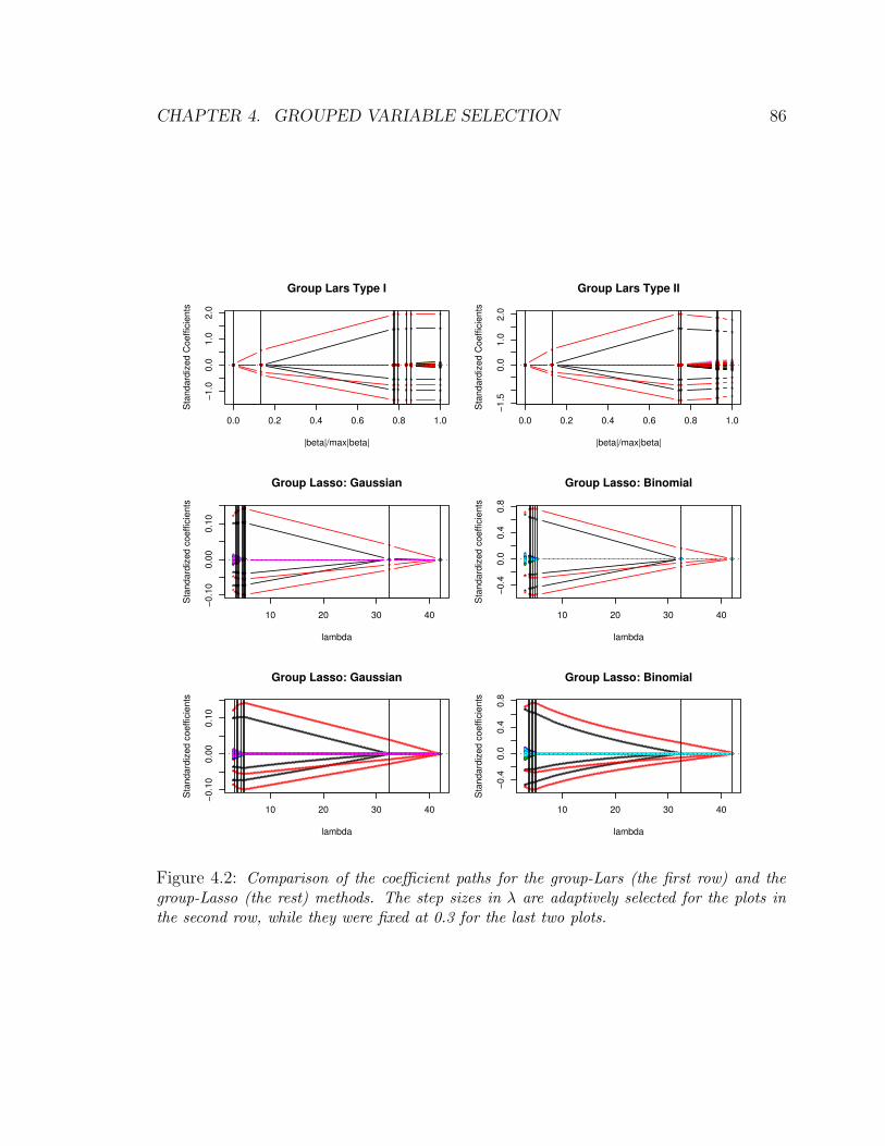
CHAPTER 4. GROUPED VARIABLE SELECTION 86
* *
*** * * *
0.0 0.2 0.4 0.6 0.8 1.0
−1.0
0.0
1.0
2.0
Group Lars Type I
|beta|/max|beta|
Sta
ndar
dize
d C
oeffi
cien
ts
* *
*** * * *
* **** * * *
*
*
*** * * *
**
*** * * *
**
*** * * *
* * *** * * ** * *** * * ** * *** * * ** * *** * * ** * *** * * ** * *** * * ** * *** * * ** * *** * * ** * *** * * ** * *** * * ** * *** * * ** * *** * * ** * *** * * ** * *** * * ** * *** * * ** * *** * * ** * *** * * ** * *** * * ** * *** * * ** * *** * * ** * *** * * ** * *** * * ** * *** * * ** * *** * * ** * *** * * ** * *** * * ** * *** * * ** * *** * * ** * *** * * ** * *** * * ** * *** * * ** * *** * * ** * *** * * ** * *** * * ** * *** * * ** * *** * * ** * *** * * ** * *** * * ** * *** * * ** * *** * * ** * *** * * ** * *** * * ** * *** * * ** * *** * * ** * *** * * * * *
*** ** *
0.0 0.2 0.4 0.6 0.8 1.0
−1.5
0.0
1.0
2.0
Group Lars Type II
|beta|/max|beta|
Sta
ndar
dize
d C
oeffi
cien
ts
* *
*** ** *
* *
*** ** **
*
*** ** *
**
*** ** *
**
*** ** *
* * *** ** ** * *** ** ** * *** ** ** * *** ** ** * *** ** ** * *** ** ** * *** ** ** * *** ** ** * *** ** ** * *** ** ** * *** ** ** * *** ** ** * *** ** ** * *** ** ** * *** ** ** * *** ** ** * *** ** ** * *** ** ** * *** ** ** * *** ** ** * *** ** ** * *** ** ** * *** ** ** * *** ** ** * *** ** ** * *** ** ** * *** ** ** * *** ** ** * *** ** ** * *** ** ** * *** ** ** * *** ** ** * *** ** ** * *** ** ** * *** ** ** * *** ** ** * *** ** ** * *** ** ** * *** ** ** * *** ** ** * *** ** ** * *** ** ** * *** ** ** * *** ** ** * *** ** *
**
**************
10 20 30 40
−0.1
00.
000.
10
lambda
Sta
ndar
dize
d co
effic
ient
s
**
**************
****************
**
**************
**
**************
**
**************
**************** **************** **************** **************** **************** **************** **************** **************** **************** **************** **************** **************** **************** **************** **************** **************** **************** **************** **************** **************** **************** **************** **************** **************** **************** **************** **************** **************** **************** **************** **************** **************** **************** **************** **************** **************** **************** **************** **************** **************** **************** **************** **************** **************** **************** **************** **************** **************** **************** **************** **************** **************** **************** **************** **************** **************** **************** **************** **************** **************** **************** **************** **************** **************** **************** **************** **************** **************** **************** **************** **************** **************** **************** **************** **************** **************** **************** **************** **************** **************** ****************
Group Lasso: Gaussian
**
*******
10 20 30 40
−0.4
0.0
0.4
0.8
lambda
Sta
ndar
dize
d co
effic
ient
s
**
*******
**
*******
**
*******
**
*******
**
*******
********* ********* ********* ********* ********* ********* ********* ********* ********* ********* ********* ********* ********* ********* ********* ********* ********* ********* ********* ********* ********* ********* ********* ********* ********* ********* ********* ********* ********* ********* ****************** ********* ********* ********* ********* ********* ********* ********* ********* ********* ********* ********* ********* ********* ********* ********* ********* ********* ********* ********* ********* ********* ********* ********* ********* ********* ********* ********* ********* ********* ********* ********* ********* ********* ********* ********* ********* ********* ********* ********* *********
Group Lasso: Binomial
**************************************************************
******************************
*****************************
***********
10 20 30 40
−0.1
00.
000.
10
lambda
Sta
ndar
dize
d co
effic
ient
s
************************************************************************************************************************************
*************************************************************************************************************************************************
***************************
******************************
******************************
********************************
************************************************************************************************************************************
************************************************************************************************************************************
************************************************************************************************************************************ ************************************************************************************************************************************ ************************************************************************************************************************************ ************************************************************************************************************************************ ************************************************************************************************************************************ ************************************************************************************************************************************ ************************************************************************************************************************************ ************************************************************************************************************************************ ************************************************************************************************************************************ ************************************************************************************************************************************ ************************************************************************************************************************************ ************************************************************************************************************************************ ************************************************************************************************************************************ ************************************************************************************************************************************ ************************************************************************************************************************************ ************************************************************************************************************************************ ************************************************************************************************************************************ ************************************************************************************************************************************ ************************************************************************************************************************************ ************************************************************************************************************************************ ************************************************************************************************************************************ ************************************************************************************************************************************ ************************************************************************************************************************************ ************************************************************************************************************************************ ************************************************************************************************************************************ ************************************************************************************************************************************ ************************************************************************************************************************************ ************************************************************************************************************************************ ************************************************************************************************************************************ ************************************************************************************************************************************ ************************************************************************************************************************************ ************************************************************************************************************************************ ************************************************************************************************************************************ ************************************************************************************************************************************ ************************************************************************************************************************************ ************************************************************************************************************************************ ************************************************************************************************************************************ ************************************************************************************************************************************ ************************************************************************************************************************************ ************************************************************************************************************************************ ************************************************************************************************************************************ ************************************************************************************************************************************ ************************************************************************************************************************************ ************************************************************************************************************************************ ************************************************************************************************************************************ ************************************************************************************************************************************ ************************************************************************************************************************************ ************************************************************************************************************************************ ************************************************************************************************************************************ ************************************************************************************************************************************ ************************************************************************************************************************************ ************************************************************************************************************************************ ************************************************************************************************************************************ ************************************************************************************************************************************ ************************************************************************************************************************************ ************************************************************************************************************************************ ************************************************************************************************************************************ ************************************************************************************************************************************ ************************************************************************************************************************************ ************************************************************************************************************************************ ************************************************************************************************************************************ ************************************************************************************************************************************ ************************************************************************************************************************************ ************************************************************************************************************************************ ************************************************************************************************************************************ ************************************************************************************************************************************ ************************************************************************************************************************************ ************************************************************************************************************************************ ************************************************************************************************************************************ ************************************************************************************************************************************ ************************************************************************************************************************************ ************************************************************************************************************************************ ************************************************************************************************************************************ ************************************************************************************************************************************ ************************************************************************************************************************************ ************************************************************************************************************************************ ************************************************************************************************************************************ ************************************************************************************************************************************ ************************************************************************************************************************************ ************************************************************************************************************************************ ************************************************************************************************************************************
Group Lasso: Gaussian
**********************************************************************
****************************
********************
**************
10 20 30 40
−0.4
0.0
0.4
0.8
lambda
Sta
ndar
dize
d co
effic
ient
s
************************************************************************************************************************************
************************************************************************************************************************************
************************************
************************************
****************************
********************
************
************************************************************************************************************************************
************************************************************************************************************************************
************************************************************************************************************************************ ************************************************************************************************************************************ ************************************************************************************************************************************ ************************************************************************************************************************************ ************************************************************************************************************************************ ************************************************************************************************************************************ ************************************************************************************************************************************ ************************************************************************************************************************************ ************************************************************************************************************************************ ************************************************************************************************************************************ ************************************************************************************************************************************ ************************************************************************************************************************************ ************************************************************************************************************************************ ************************************************************************************************************************************ ************************************************************************************************************************************ ************************************************************************************************************************************ ************************************************************************************************************************************ ************************************************************************************************************************************ ************************************************************************************************************************************ ************************************************************************************************************************************ ************************************************************************************************************************************ ************************************************************************************************************************************ ************************************************************************************************************************************ ************************************************************************************************************************************ ************************************************************************************************************************************ ************************************************************************************************************************************ ************************************************************************************************************************************ ************************************************************************************************************************************ ************************************************************************************************************************************ ************************************************************************************************************************************ ************************************************************************************************************************************************************************************************************************************************************************ ************************************************************************************************************************************ ************************************************************************************************************************************ ************************************************************************************************************************************ ************************************************************************************************************************************ ************************************************************************************************************************************ ************************************************************************************************************************************ ************************************************************************************************************************************ ************************************************************************************************************************************ ************************************************************************************************************************************ ************************************************************************************************************************************ ************************************************************************************************************************************ ************************************************************************************************************************************ ************************************************************************************************************************************ ************************************************************************************************************************************ ************************************************************************************************************************************ ************************************************************************************************************************************ ************************************************************************************************************************************ ************************************************************************************************************************************ ************************************************************************************************************************************ ************************************************************************************************************************************ ************************************************************************************************************************************ ************************************************************************************************************************************ ************************************************************************************************************************************ ************************************************************************************************************************************ ************************************************************************************************************************************ ************************************************************************************************************************************ ************************************************************************************************************************************ ************************************************************************************************************************************ ************************************************************************************************************************************ ************************************************************************************************************************************ ************************************************************************************************************************************ ************************************************************************************************************************************ ************************************************************************************************************************************ ************************************************************************************************************************************ ************************************************************************************************************************************ ************************************************************************************************************************************ ************************************************************************************************************************************ ************************************************************************************************************************************ ************************************************************************************************************************************ ************************************************************************************************************************************
Group Lasso: Binomial
Figure 4.2: Comparison of the coefficient paths for the group-Lars (the first row) and thegroup-Lasso (the rest) methods. The step sizes in λ are adaptively selected for the plots inthe second row, while they were fixed at 0.3 for the last two plots.

CHAPTER 4. GROUPED VARIABLE SELECTION 87
exact paths with a reasonable accuracy by adjusting the step lengths as illustrated in
Section 4.2.3, thereby significantly reducing the total number of iterations (132 to 16
for the Gaussian, and 132 to 9 for the binomial case).
4.4 Real Data Example
We applied the path-following procedures and stepwise logistic regression with L2
penalization to a real dataset with genotype measurements on 14 loci and a binary
response indicating the presence of bladder cancer (201 cases and 214 controls). The
dataset was first introduced in Hung et al. (2004).
Table 4.3 summarizes the cross-validated prediction error, sensitivity, and speci-
ficity from a five-fold cross-validation. For each fold, we ran an internal cross-validation
to choose the level of regularization. The negative log-likelihood was used as the crite-
rion in the internal cross-validations. Overall (classification) error rate was the lowest
for stepwise logistic regression, the specificity being especially high compared to other
methods.
Methods Prediction error Sensitivity Specificity
Group-Lars I 156/415=0.376 128/201 131/214Group-Lars II 155/415=0.373 127/201 133/214
Group-Lasso (Gaussian) 154/415=0.371 126/201 135/214Group-Lasso (Binomial) 157/415=0.378 128/201 130/214
Step PLR 147/415=0.354 122/201 146/214
Table 4.3: Comparison of prediction performances
One would expect an improvement by applying a smooth variable selection mecha-
nism as in group-Lars or group-Lasso. However, such smoothness may turn out to be a
disadvantage. As in Section 4.3, the group-Lars and the group-Lasso methods tend to
select irrelevant terms more easily than stepwise logistic regression. Even when these
path-following methods identify a correct subset of features, the nonzero coefficients

CHAPTER 4. GROUPED VARIABLE SELECTION 88
0.0 0.2 0.4 0.6 0.8 1.0
0.0
0.2
0.4
0.6
0.8
1.0
ROC curves: group Lars, PLR
specificity
sens
itivi
ty
PLRgLars:Type IgLars:Type II
0.0 0.2 0.4 0.6 0.8 1.0
0.0
0.2
0.4
0.6
0.8
1.0
ROC curves: group Lasso, PLR
specificity
sens
itivi
ty
PLRgLasso:GaussiangLasso:Binomial
Figure 4.3: Comparison of ROC curves
are shrunken fits. On the other hand, the L2 regularization in our stepwise logistic
regression is meaningful as a technical device (Chapter 2) rather than as a smoothing
tool, and thus, we often apply only a slight penalization to the size of the coefficients.
We further extended the prediction error analysis by plotting the receiver operating
characteristic (ROC) curves for all the methods compared in Table 4.3. For each
method, we generated multiple sets of classification results by applying different cut-
off values to the cross-validated responses from the previous analysis. The left and
right panels of Figure 4.3 compare the ROC curves of the group-Lars methods and
the group-Lasso methods to stepwise logistic regression, respectively. The ROC curve
for stepwise logistic regression lies slightly more toward the upper right-hand corner
than all the other curves, although the difference is not statistically significant.

CHAPTER 4. GROUPED VARIABLE SELECTION 89
4.5 Summary
In this chapter, we studied the use of various regularization path algorithms for
grouped variable selection to fit gene-interaction models. We first considered two
types of group-Lars algorithms. Group-Lars Type I, proposed by Yuan & Lin (2006),
kept the groups with the largest average squared correlation with the current residu-
als in the active set. In group-Lars Type II, the active groups were the ones with the
largest average absolute correlation. We showed some simulation results in which the
Type II algorithm was preferred because the Type I algorithm selected large groups
too easily. We then studied the group-Lasso method and suggested a general path-
following algorithm that can be implemented with the log-likelihood of any distribution
in exponential family. Although the path-algorithm for group-Lasso is more complex
than that of group-Lars, group-Lasso is more informative in that we have the explicit
criterion as in (4.3).
Group-Lasso may yield a stable fit even when highly correlated variables are input
simultaneously. When some variables are perfectly correlated within a group, as in the
case of over-represented groups of indicators for categorical factors, the solution for
group-Lasso is still uniquely determined. This property of the group-Lasso method
makes it more attractive as a way to fit with categorical factors coded in dummy
variables. On the other hand, the group-Lars paths are not unique in this situation,
and as a remedy, we used the LARS-EN algorithm with a slight L2 penalization instead
of Lars. This modification adds a quadratic feature to the group-Lars method, as in
the group-Lasso criterion.
We compared the performance of the group-Lars and the group-Lasso methods to
that of the forward stepwise approach, a more conventional variable selection strategy,
implemented with L2 penalized logistic regression. The group-Lars and the group-
Lasso methods can be preferred for being smooth in selecting terms and being faster.

CHAPTER 4. GROUPED VARIABLE SELECTION 90
However, based on our experiments, we learned that L2 penalized logistic regression
with the forward stepwise variable selection scheme is still comparable to those alter-
natives.

Chapter 5
Conclusion
As discussed earlier, fitting with high-dimensional data requires flexible modeling
strategies. Many of the conventional regression/classification schemes result in a fit
with large variance or technically do not tolerate a large number of input features.
Here we focused on adding a regularization through the size of the coefficients, which
often yields a model with larger bias but smaller variance.
The L2 norm constraint as in ridge regression (1.1) and the L1 norm constraint as
in Lasso (1.2) both in general improve the unregularized fit by reducing the variance.
However, the correlations among the features affect the relative size of each coefficient
differently in these two types of penalization. In this thesis, we suggested ways to take
advantage of the different regularization schemes for solving different problems.
The main contributions of this thesis are as follows:
• We introduced the quadratic penalization as an essential device in an application
of modeling gene-gene interactions. In such models, many variables are strongly
correlated because of the binary coding of the factors/interactions of the factors;
moreover, some variables may be zero across all the samples. As we explained
in detail in Chapter 2, the L2 penalty term in logistic regression handled these
91

CHAPTER 5. CONCLUSION 92
situations gracefully. We implemented L2 penalized logistic regression with our
modified forward stepwise variable selection procedure.
• We proposed an L1 regularization path algorithm for generalized linear models.
The paths are piecewise linear only in the case of Gaussian distribution, for
which our algorithm is equivalent to the Lars-Lasso algorithm (Efron et al. 2004).
When many redundant or noisy features exist in the data, the L1 constraint in
effect identifies a subset of significant factors, assigning them nonzero coefficients.
In Chapter 3, we demonstrated the logistic regression path with microarray data
of over 7000 genes. Our GLM path algorithm not only provided an efficient way
to model L1 regularized GLM, but also suggested a general scheme for tracing
nonlinear coefficient paths.
• Relating to both of the two previous approaches, we presented several differ-
ent strategies to fit with categorical variables and high-order interactions among
them. The group-Lars and the group-Lasso methods (Yuan & Lin 2006) pro-
vide a smoother grouped feature selection than the forward stepwise scheme
that we implemented along with L2 penalized logistic regression. Extending the
path-following strategy of the GLM path, we proposed a similar algorithm for
fitting the regularization path for group-Lasso. We also proposed another ver-
sion of group-Lars. We applied our group-Lasso (predictor-corrector) algorithm
as well as group-Lars to the data with genotype measurements, as we did earlier
with stepwise logistic regression. Through these experiments, we learned that
although stepwise logistic regression searches for the optimal model in a greedy
manner, it is as successful as other smoother path algorithms with grouped vari-
able selection.
Datasets containing categorical factors are common in many fields, and we would
like to conclude with some suggestions for making our approaches for such data more

CHAPTER 5. CONCLUSION 93
flexible. Both the forward stepwise variable selection and the group-Lasso methods
assign nonzero coefficients to all the elements of the selected groups. However, when
the number of levels of the categorical factors is large, it can be more sensible to make
the coefficients of some of the elements in the selected groups zero. Alternatively, one
can modify the criterion so that the elements in a group are automatically divided
into sub-groups within which the coefficients are forced to be the same.

Bibliography
Allgower, E. & Georg, K. (1990), Numerical Continuation Methods, Springer-Verlag,
Berlin Heidelberg.
Boyd, S. & Vandenberghe, L. (2004), Convex Optimization, Cambridge University
Press, Cambridge.
Coffey, C., Hebert, P., Ritchie, M., Krumholz, H., Gaziano, J., Ridker, P., Brown, N.,
Vaughan, D. & Moore, J. (2004), ‘An application of conditional logistic regression
and multifactor dimensionality reduction for detecting gene-gene interactions on
risk of myocardial infarction: The importance of model validation’, BMC Bioin-
formatics 5, 49.
Cox, D. (1972), ‘Regression models and life-tables’, Journal of the Royal Statistical
Society. Series B 34, 187–220.
Crowley, J. & Hu, M. (1977), ‘Covariance analysis of heart transplant survival data’,
Journal of the American Statistical Association 72, 27–36.
Donoho, D., Johnstone, I., Kerkyacharian, G. & Picard, D. (1995), ‘Wavelet shrinkage:
asymptopia?’, Journal of the Royal Statistical Society, Series B 57, 301–337.
Efron, B., Hastie, T., Johnstone, I. & Tibshirani, R. (2004), ‘Least angle regression’,
Annals of Statistics 32, 407–499.
94

BIBLIOGRAPHY 95
Efron, B. & Tibshirani, R. (1993), An Introduction to the Bootstrap, CHAPMAN &
HALL/CRC, Boca Raton.
Friedman, J. (1991), ‘Multivariate adaptive regression splines’, The Annals of Statis-
tics 19, 1–67.
Garcia, C. & Zangwill, W. (1981), Pathways to Solutions, Fixed Points and Equilibria,
Prentice-Hall, Inc., Englewood Cliffs.
Genkin, A., Lewis, D. & Madigan, D. (2004), Large-scale bayesian logistic regression
for text categorization, Technical report, Rutgers University.
Golub, T., Slonim, D., Tamayo, P., Huard, C., Gaasenbeek, M., Mesirov, J., Coller,
H., Loh, M., Downing, J., Caligiuri, M., Bloomfield, C. & Lander, E. (1999),
‘Molecular classification of cancer: Class discovery and class prediction by gene
expression monitoring’, Science 286, 531–537.
Gray, R. (1992), ‘Flexible methods for analyzing survival data using splines, with
applications to breast cancer prognosis’, Journal of the American Statistical As-
sociation 87, 942–951.
Hahn, L., Ritchie, M. & Moore, J. (2003), ‘Multifactor dimensionality reduction soft-
ware for detecting gene-gene and gene-environment interaction’, Bioinformatics
19, 376–382.
Hastie, T., Rosset, S., Tibshirani, R. & Zhu, J. (2004), ‘The entire regularization path
for the support vector machine’, Journal of Machine Learning Research 5, 1391–
1415.
Hastie, T. & Tibshirani, R. (1990), Generalized Additive Models, CHAPMAN &
HALL/CRC, London.

BIBLIOGRAPHY 96
Hastie, T., Tibshirani, R. & Friedman, J. (2001), Elements of Statistical Learning;
Data Mining, Inference, and Prediction, Springer-Verlag, New York.
Hoerl, A. E. & Kennard, R. (1970), ‘Ridge regression: Biased estimation for
nonorthogonal problems’, Technometrics 12, 55–67.
Huang, J., Lin, A., Narasimhan, B., Quertermous, T., Hsiung, C., Ho, L., Grove,
J., Oliver, M., Ranade, K., Risch, N. & Olshen, R. (2004), ‘Tree-structured su-
pervised learning and the genetics of hypertension’, Proceedings of the National
Academy of Sciences 101, 10529–10534.
Hung, R., Brennan, P., Malaveille, C., Porru, S., Donato, F., Boffetta, P. & Witte,
J. (2004), ‘Using hierarchical modeling in genetic association studies with mul-
tiple markers: Application to a case-control study of bladder cancer’, Cancer
Epidemiology, Biomarkers & Prevention 13, 1013–1021.
Le Cessie, S. & Van Houwelingen, J. (1992), ‘Ridge estimators in logistic regression’,
Applied Statistics 41, 191–201.
Lee, A. & Silvapulle, M. (1988), ‘Ridge estimation in logistic regression’, Communi-
cations in Statistics, Simulation and Computation 17, 1231–1257.
McCullagh, P. & Nelder, J. (1989), Generalized Linear Models, CHAPMAN &
HALL/CRC, Boca Raton.
Meier, L., van de Geer, S. & Buhlmann, P. (2006), The group lasso for logistic regres-
sion, Technical report, Eidgenossische Technische Hochschule Zurich, Zurich.
Munkres, J. (1991), Analysis on Manifolds, Addison-Wesley Publishing Company,
Reading.

BIBLIOGRAPHY 97
Neuman, R. & Rice, J. (1992), ‘Two-locus models of disease’, Genetic Epidemiology
9, 347–365.
Osborne, M., Presnell, B. & Turlach, B. (2000), ‘On the lasso and its dual’, Journal
of Computational and Graphical Statistics 9, 319–337.
Risch, N. (1990), ‘Linkage strategies for genetically complex traits. i. multilocus mod-
els’, American Journal of Human Genetics 46, 222–228.
Ritchie, M., Hahn, L. & Moore, J. (2003), ‘Power of multifactor dimensionality re-
duction for detecting gene-gene interactions in the presence of genotyping er-
ror, missing data, phenocopy, and genetic heterogeneity’, Genetic Epidemiology
24, 150–157.
Ritchie, M., Hahn, L., Roodi, N., Bailey, L., Dupont, W., Parl, F. & Moore,
J. (2001), ‘Multifactor-dimensionality reduction reveals high-order interactions
among estrogen-metabolism genes in sporadic breast cancer’, American Journal
of Human Genetics 69, 138–147.
Rosset, S. (2004), Tracking curved regularized optimization solution paths, in ‘Neural
Information Processing Systems’.
Rosset, S. & Zhu, J. (2004), Piecewise linear regularized solution paths, Technical
report, Stanford University.
Rosset, S., Zhu, J. & Hastie, T. (2004), ‘Boosting as a regularized path to a maximum
margin classifier’, Journal of Machine Learning Research 5, 941–973.
Shevade, S. & Keerthi, S. (2003), ‘A simple and efficient algorithm for gene selection
using sparse logistic regression’, Bioinformatics 19, 2246–2253.

BIBLIOGRAPHY 98
Speed, T. (2003), Statistical Analysis of Gene Expression Microarray Data, Chapman
& HallCRC, London.
Stein, C. (1981), ‘Estimation of the mean of a multivariate normal distribution’, An-
nals of Statistics 9, 1135–1151.
Tibshirani, R. (1996), ‘Regression shrinkage and selection via the lasso’, Journal of
the Royal Statistical Society. Series B 58, 267–288.
Tibshirani, R. (1997), ‘The lasso method for variable selection in the cox model’,
Statistics in Medicine 16, 385–395.
Tibshirani, R., Hastie, T., Narasimhan, B. & Chu, G. (2002), ‘Diagnosis of multi-
ple cancer types by shrunken centroids of gene expression’, Proceedings of the
National Academy of Sciences 99, 6567–6572.
Vieland, V. & Huang, J. (2003), ‘Two-locus heterogeneity cannot be distinguished
from two-locus epistasis on the basis of affected-sib-pair data’, American Journal
of Human Genetics 73, 223–232.
Wit, E. & McClure, J. (2004), Statistics for Microarrays: Design, Analysis and Infer-
ence, John Wiley & Sons Ltd., Chichester.
Yuan, M. & Lin, Y. (2006), ‘Model selection and estimation in regression with grouped
variables’, Journal of the Royal Statistical Society. Series B 68, 49–67.
Zhao, P. & Yu, B. (2004), Boosted lasso, Technical report, University of California,
Berkeley.
Zhu, J. & Hastie, T. (2004), ‘Classification of gene microarrays by penalized logistic
regression’, Biostatistics 46, 505–510.

BIBLIOGRAPHY 99
Zhu, J., Rosset, S., Hastie, T. & Tibshirani, R. (2003), 1-norm support vector ma-
chines, in ‘Neural Information Processing Systems’.
Zou, H. & Hastie, T. (2004), On the ”degrees of freedom” of the lasso, Technical
report, Stanford University.
Zou, H. & Hastie, T. (2005), ‘Regularization and variable selection via the elastic net’,
Journal of the Royal Statistical Society. Series B 67, 301–320.


