0.5
setg
ray0
0.5
setg
ray1
Genetic Algorithms and GeneticProgramming
Pavia University and INFNThird Lecture: Application to HEP
Eric W. [email protected]
Vanderbilt University
Eric Vaandering – Genetic Programming, # 3 – p. 1/40
Overview• Machine learning techniques• Genetic Algorithms• Genetic Programming
• Review• Application to a problem in HEP
Eric Vaandering – Genetic Programming, # 3 – p. 2/40
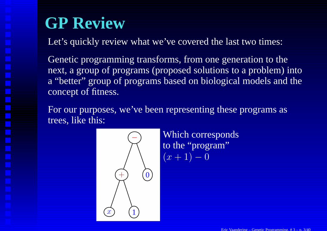
GP ReviewLet’s quickly review what we’ve covered the last two times:
Genetic programming transforms, from one generation to thenext, a group of programs (proposed solutions to a problem) intoa “better” group of programs based on biological models and theconcept of fitness.
For our purposes, we’ve been representing these programs astrees, like this:
−
+
x 1
0
Which correspondsto the “program”(x + 1) − 0
Eric Vaandering – Genetic Programming, # 3 – p. 3/40

“Running” the GPWith what we learned last time, we are ready to “run” the GP(i.e. find a solution). Recall that these are the steps a GPframework will take:
• User has defined functions and definition of fitness• Generate a population of programs (few hundred to few
thousand) to be tested• Test each program against fitness definition• Choose genetic operation (copy, crossover, or mutation)
and individuals to create next generation• Chosen randomly according to fitness
• Repeat process for next generation• Often tens of generations are needed to find the best
solution• At the end, we have a large number of solutions; we look at
the best fewEric Vaandering – Genetic Programming, # 3 – p. 4/40

Parallelizing the GPEach test takes a while (10–60 sec on a 2 GHz P4) so spread overmultiple computers
• Adopt a South Pacific island type model• A population on each island (CPU)• Every few generations, migrate the best individuals
from each island to each other island• Lots of parameters to be tweaked, like size of programs,
probabilities of reproduction methods, exchanges, etc.• None of them seem to matter all that much, process is
robust
Eric Vaandering – Genetic Programming, # 3 – p. 5/40

Parallelizing the GP
Eric Vaandering – Genetic Programming, # 3 – p. 6/40
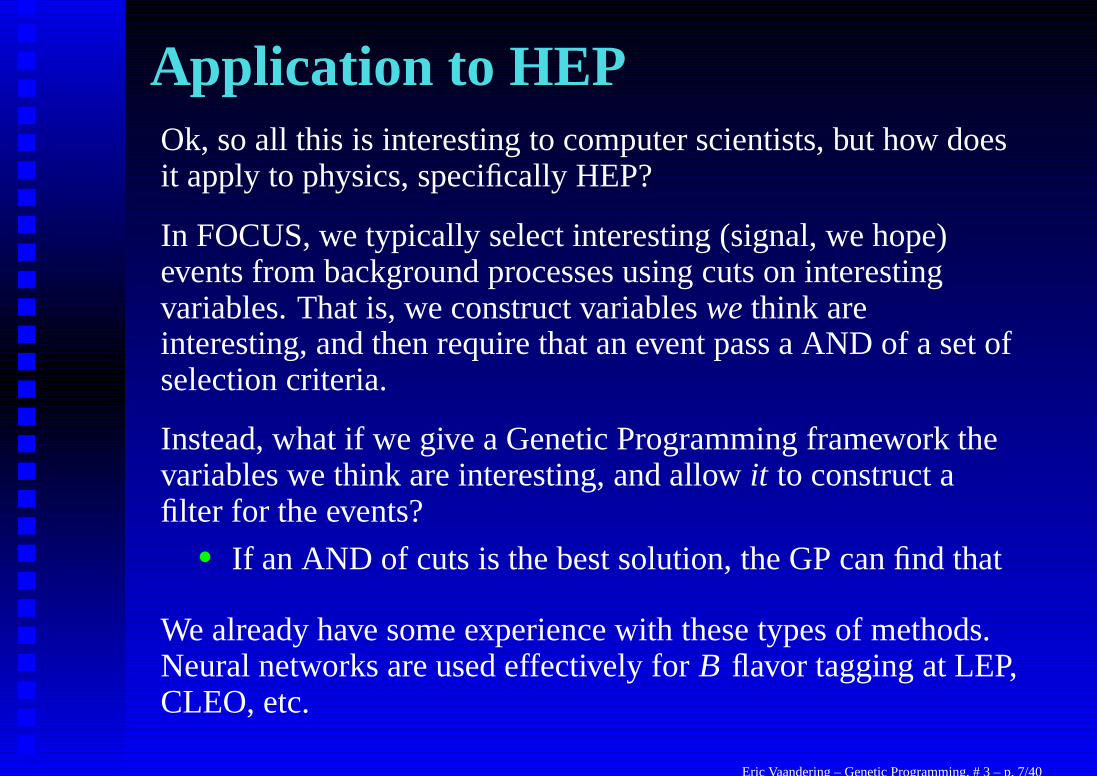
Application to HEPOk, so all this is interesting to computer scientists, but how doesit apply to physics, specifically HEP?
In FOCUS, we typically select interesting (signal, we hope)events from background processes using cuts on interestingvariables. That is, we construct variables we think areinteresting, and then require that an event pass a AND of a set ofselection criteria.
Instead, what if we give a Genetic Programming framework thevariables we think are interesting, and allow it to construct afilter for the events?
• If an AND of cuts is the best solution, the GP can find that
We already have some experience with these types of methods.Neural networks are used effectively for B flavor tagging at LEP,CLEO, etc.
Eric Vaandering – Genetic Programming, # 3 – p. 7/40
What’s it good for?• Replace or supplement cuts• Allow us to include indicators of interesting decays in the
selection process• These indicators can include variables we can’t cut on
(too low efficiency)• Can form correlations we might not think of
• Has already had this benefit
Eric Vaandering – Genetic Programming, # 3 – p. 8/40
QuestionsWhen considering an approach like this, some questionsnaturally arise:
• How do we know it’s not biased?• The tree can grow large with useless information.• Does it do as well as normal cut methods do?• Is it evolving or randomly finding good combinations?• What about units? Can you add a momentum and a mass?
• All numbers are defined to be unit-less
Eric Vaandering – Genetic Programming, # 3 – p. 9/40
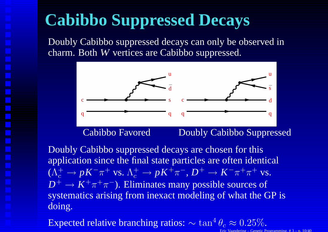
Cabibbo Suppressed DecaysDoubly Cabibbo suppressed decays can only be observed incharm. Both W vertices are Cabibbo suppressed.
q
c
q
s
d̄
u
q
c
q
d
s̄
u
Cabibbo Favored Doubly Cabibbo Suppressed
Doubly Cabibbo suppressed decays are chosen for thisapplication since the final state particles are often identical(Λ+
c → pK−π+ vs. Λ+c → pK+π−, D+ → K−π+π+ vs.
D+ → K+π+π−). Eliminates many possible sources ofsystematics arising from inexact modeling of what the GP isdoing.
Expected relative branching ratios: ∼ tan4 θc ≈ 0.25%.Eric Vaandering – Genetic Programming, # 3 – p. 10/40
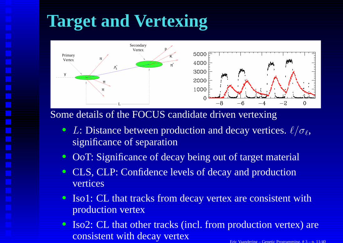
Target and Vertexing
π
L
Λ
-
c+
+
π
π
π
γ
Vertex
SecondaryVertex
Primary Κ
p
Some details of the FOCUS candidate driven vertexing• L: Distance between production and decay vertices. `/σ`,
significance of separation• OoT: Significance of decay being out of target material• CLS, CLP: Confidence levels of decay and production
vertices• Iso1: CL that tracks from decay vertex are consistent with
production vertex• Iso2: CL that other tracks (incl. from production vertex) are
consistent with decay vertexEric Vaandering – Genetic Programming, # 3 – p. 11/40
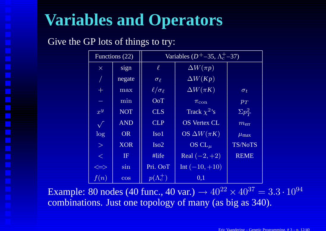
Variables and OperatorsGive the GP lots of things to try:
Functions (22) Variables (D+–35, Λ+c –37)
× sign ` ∆W (πp)
/ negate σ` ∆W (Kp)
+ max `/σ` ∆W (πK) σt
− min OoT πcon pT
xy NOT CLS Track χ2’s Σp2T
√ AND CLP OS Vertex CL merr
log OR Iso1 OS ∆W (πK) µmax
> XOR Iso2 OS CLµ TS/NoTS
< IF #life Real (−2, +2) REME
<=> sin Pri. OoT Int (−10, +10)
f(n) cos p(Λ+c ) 0,1
Example: 80 nodes (40 func., 40 var.) → 4022 × 4037 = 3.3 · 1094
combinations. Just one topology of many (as big as 340).
Eric Vaandering – Genetic Programming, # 3 – p. 12/40

Evaluating the GPFor each program the GP framework suggests, we have to tell theframework how good the program is:
• All functions must be well defined for all input values, so> → 1 (true) or 0 (false), log of neg. number, etc.
• Evaluate the tree for each event, which gives a single value• Select events for which Tree > 0
• Initial sample has as loose cuts as possible• Return a fitness to framework• Could be ∝
√S + B/S (framework wants to minimize)
• In this case S is from CF mode scaled down toexpected/measured DCS level. B is from fit to DCS BG(masking out signal region if appropriate).
Eric Vaandering – Genetic Programming, # 3 – p. 13/40
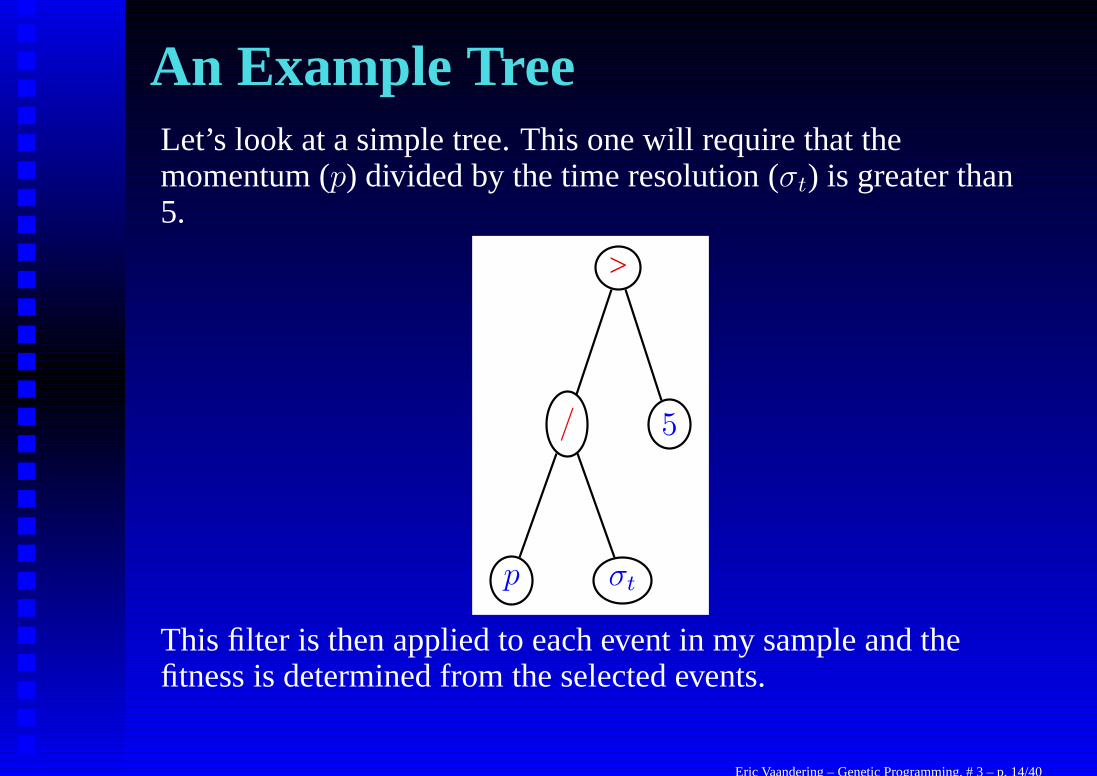
An Example TreeLet’s look at a simple tree. This one will require that themomentum (p) divided by the time resolution (σt) is greater than5.
>
/
p σt
5
This filter is then applied to each event in my sample and thefitness is determined from the selected events.
Eric Vaandering – Genetic Programming, # 3 – p. 14/40

Λ+c → pK+π−
The first decay we’re looking for is Λ+c → pK+π−. There are no
observations or limits. Even an observation of tan4 θc relative toΛ+
c → pK−π+ is challenging, but there is a complication.
The Cabibbo favored mode has an W -exchange contributionwhile the DCS decay does not. (This contribution is also why theΛ+
c lifetime is about one half the Ξ+c lifetime.)
u
d
c
u
u
q
q
s
So, the expected branching ratio will be reduced, maybe by 50%.
Eric Vaandering – Genetic Programming, # 3 – p. 15/40
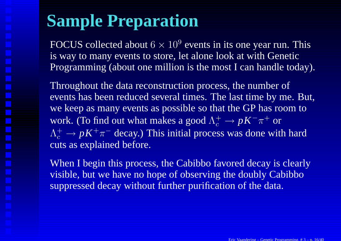
Sample PreparationFOCUS collected about 6 × 10⁹ events in its one year run. Thisis way to many events to store, let alone look at with GeneticProgramming (about one million is the most I can handle today).
Throughout the data reconstruction process, the number ofevents has been reduced several times. The last time by me. But,we keep as many events as possible so that the GP has room towork. (To find out what makes a good Λ+
c → pK−π+ orΛ+
c → pK+π− decay.) This initial process was done with hardcuts as explained before.
When I begin this process, the Cabibbo favored decay is clearlyvisible, but we have no hope of observing the doubly Cabibbosuppressed decay without further purification of the data.
Eric Vaandering – Genetic Programming, # 3 – p. 16/40
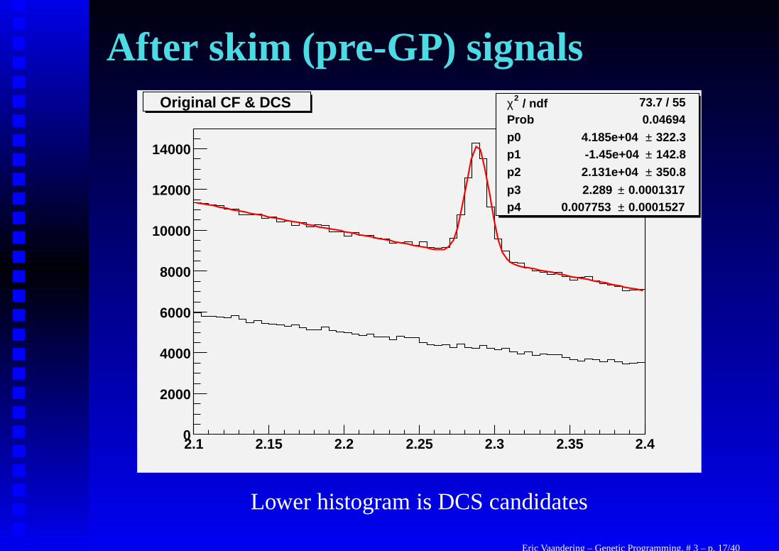
After skim (pre-GP) signals / ndf 2χ 73.7 / 55
Prob 0.04694p0 322.3± 4.185e+04 p1 142.8± -1.45e+04 p2 350.8± 2.131e+04
p3 0.0001317± 2.289 p4 0.0001527± 0.007753
2.1 2.15 2.2 2.25 2.3 2.35 2.40
2000
4000
6000
8000
10000
12000
14000
/ ndf 2χ 73.7 / 55Prob 0.04694p0 322.3± 4.185e+04 p1 142.8± -1.45e+04 p2 350.8± 2.131e+04
p3 0.0001317± 2.289 p4 0.0001527± 0.007753
Original CF & DCS
Lower histogram is DCS candidates
Eric Vaandering – Genetic Programming, # 3 – p. 17/40
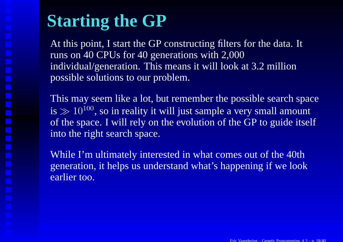
Starting the GPAt this point, I start the GP constructing filters for the data. Itruns on 40 CPUs for 40 generations with 2,000individual/generation. This means it will look at 3.2 millionpossible solutions to our problem.
This may seem like a lot, but remember the possible search spaceis � 10100, so in reality it will just sample a very small amountof the space. I will rely on the evolution of the GP to guide itselfinto the right search space.
While I’m ultimately interested in what comes out of the 40thgeneration, it helps us understand what’s happening if we lookearlier too.
Eric Vaandering – Genetic Programming, # 3 – p. 18/40

Size (Parsimony) PressureAn aside: I apply a penalty to the fitness for each node in thetree. This is to try to keep the tree sizes small. This is notrecommended by the literature:
• How do you know the right penalty?• Maybe you miss out on some subtree that needs to grow
over time• Not really shown to help
Never the less, I still do it. Why?• Reduces execution time• Worry about training the GP to recognize individual events• Better chance to understand final trees
The penalty I assess is 0.5% per node. That is, a 101-node treehas its fitness increased by 50% over single node tree thatperforms as well.
Eric Vaandering – Genetic Programming, # 3 – p. 19/40
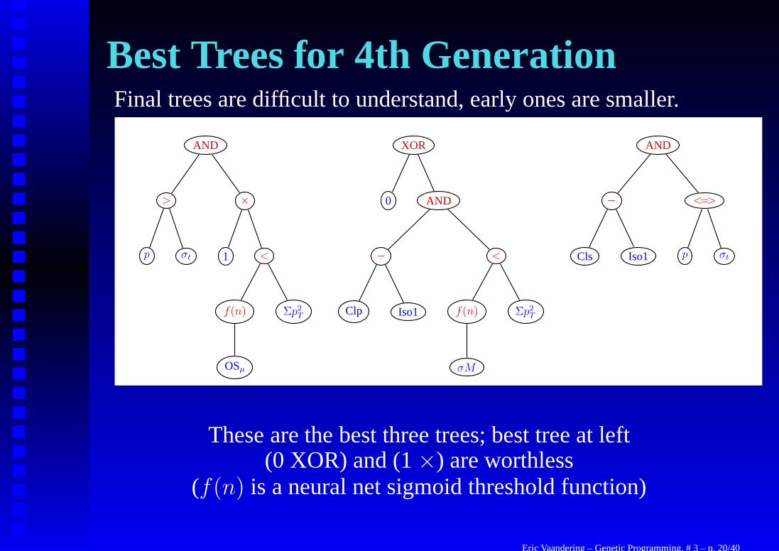
Best Trees for 4th GenerationFinal trees are difficult to understand, early ones are smaller.
AND
>
p σt
×
1 <
f(n)
OSµ
Σp2T
XOR
0 AND
−
Clp Iso1
<
f(n)
σM
Σp2T
AND
−
Cls Iso1
<=>
p σt
These are the best three trees; best tree at left(0 XOR) and (1 ×) are worthless
(f(n) is a neural net sigmoid threshold function)
Eric Vaandering – Genetic Programming, # 3 – p. 20/40
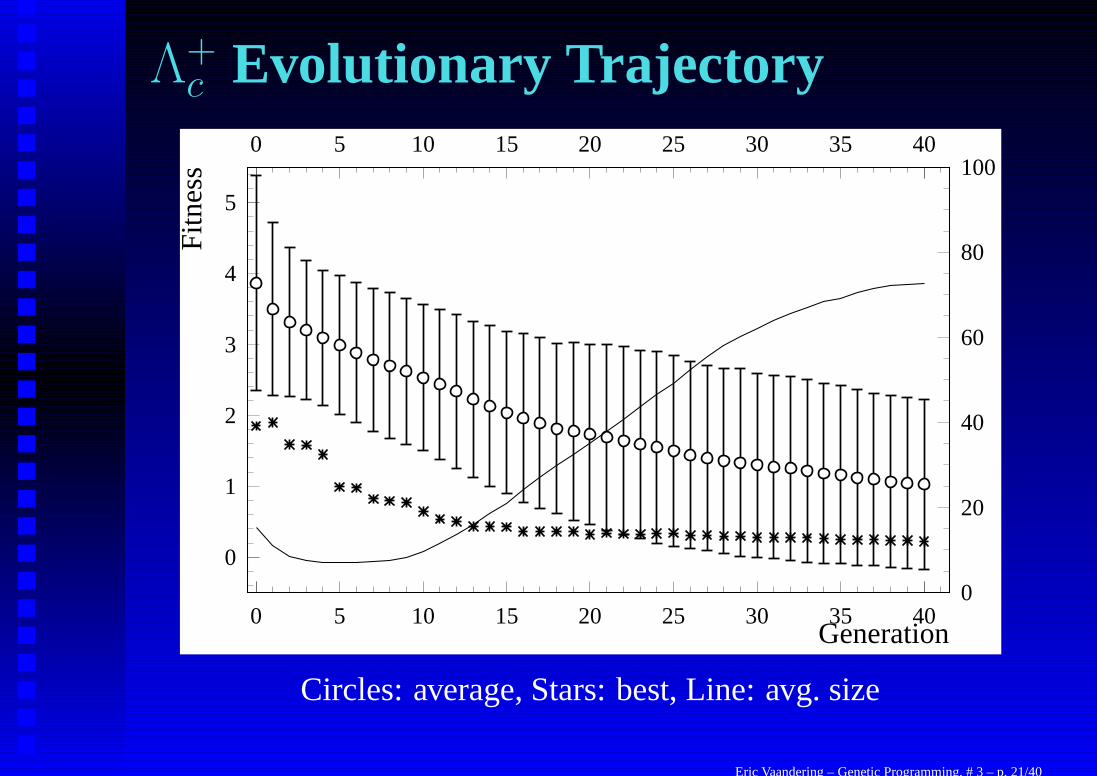
Λ+c Evolutionary Trajectory
0
1
2
3
4
5
0 5 10 15 20 25 30 35 40Generation
Fitn
ess
0
20
40
60
80
1000 5 10 15 20 25 30 35 40
Circles: average, Stars: best, Line: avg. size
Eric Vaandering – Genetic Programming, # 3 – p. 21/40

Expansion of best trees
0.2
0.22
0.24
0.26
0.28
0.3
0.32
0.34
0.36
0.38
0.4
0 5 10 15 20 25 30 35 40
Stars are the best tree, still evolving at generation 40
Eric Vaandering – Genetic Programming, # 3 – p. 22/40
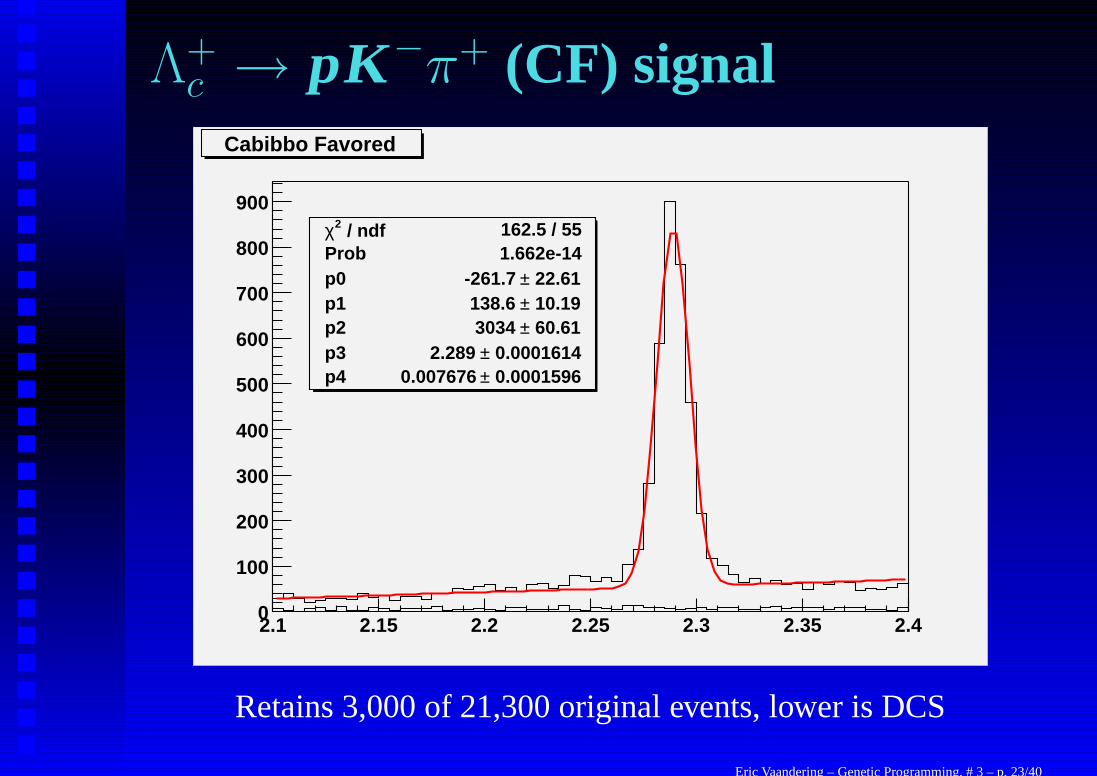
Λ+c → pK−π+ (CF) signal
/ ndf 2χ 162.5 / 55Prob 1.662e-14p0 22.61± -261.7 p1 10.19± 138.6 p2 60.61± 3034 p3 0.0001614± 2.289 p4 0.0001596± 0.007676
2.1 2.15 2.2 2.25 2.3 2.35 2.40
100
200
300
400
500
600
700
800
900 / ndf 2χ 162.5 / 55
Prob 1.662e-14p0 22.61± -261.7 p1 10.19± 138.6 p2 60.61± 3034 p3 0.0001614± 2.289 p4 0.0001596± 0.007676
Cabibbo Favored
Retains 3,000 of 21,300 original events, lower is DCS
Eric Vaandering – Genetic Programming, # 3 – p. 23/40

Λ+c → pK+π− (DCS) signal
/ ndf 2χ 73.07 / 57Prob 0.07432p0 6.417± -9.228 p1 2.865± 7.375 p2 7.137± 1.093 p3 0± 2.289 p4 0± 0.007676
2.1 2.15 2.2 2.25 2.3 2.35 2.40
2
4
6
8
10
12
14
/ ndf 2χ 73.07 / 57Prob 0.07432p0 6.417± -9.228 p1 2.865± 7.375 p2 7.137± 1.093 p3 0± 2.289 p4 0± 0.007676
DCS
Mass and width are fixed to CF values
Eric Vaandering – Genetic Programming, # 3 – p. 24/40
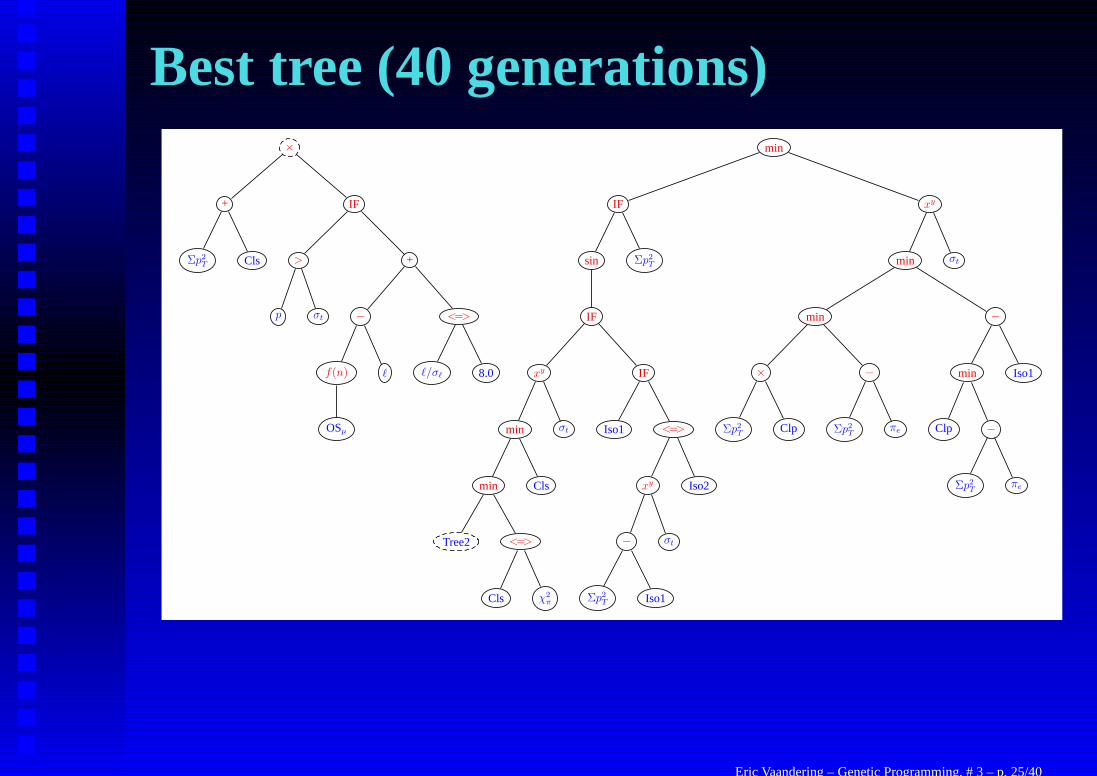
Best tree (40 generations)×
+
Σp2T Cls
IF
>
p σt
+
−
f(n)
OSµ
`
<=>
`/σ` 8.0
min
IF
sin
IF
xy
min
min
Tree2 <=>
Cls χ2π
Cls
σt
IF
Iso1 <=>
xy
−
Σp2T Iso1
σt
Iso2
Σp2T
xy
min
min
×
Σp2T Clp
−
Σp2T
πe
−
min
Clp −
Σp2T
πe
Iso1
σt
Eric Vaandering – Genetic Programming, # 3 – p. 25/40
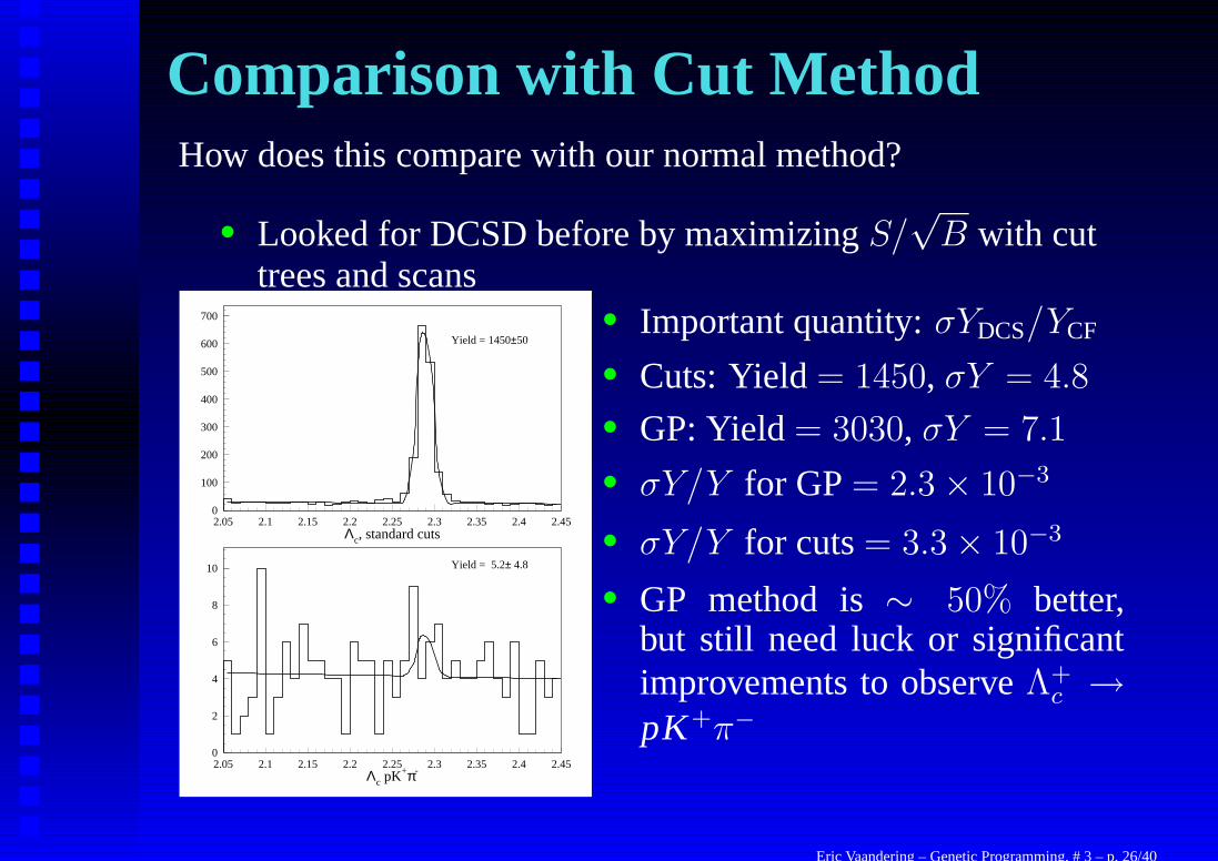
Comparison with Cut MethodHow does this compare with our normal method?
• Looked for DCSD before by maximizing S/√
B with cuttrees and scans
Λc, standard cuts
0
100
200
300
400
500
600
700
2.05 2.1 2.15 2.2 2.25 2.3 2.35 2.4 2.45
Yield = 1450±50
Λc pK+π-
0
2
4
6
8
10
2.05 2.1 2.15 2.2 2.25 2.3 2.35 2.4 2.45
Yield = 5.2± 4.8
• Important quantity: σYDCS/YCF
• Cuts: Yield = 1450, σY = 4.8
• GP: Yield = 3030, σY = 7.1
• σY/Y for GP = 2.3 × 10⁻³
• σY/Y for cuts = 3.3 × 10⁻³
• GP method is ∼ 50% better,but still need luck or significantimprovements to observe Λ+
c →pK+π−
Eric Vaandering – Genetic Programming, # 3 – p. 26/40
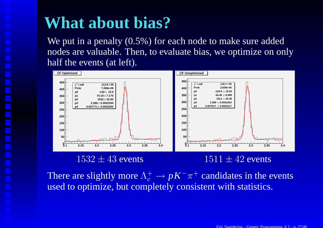
What about bias?We put in a penalty (0.5%) for each node to make sure addednodes are valuable. Then, to evaluate bias, we optimize on onlyhalf the events (at left).
/ ndf 2χ 112.8 / 55Prob 7.269e-06p0 15.9± -142 p1 7.175± 74.18 p2 42.93± 1532 p3 0.0002294± 2.289 p4 0.0002292± 0.007771
2.1 2.15 2.2 2.25 2.3 2.35 2.40
50
100
150
200
250
300
350
400
450 / ndf 2χ 112.8 / 55
Prob 7.269e-06p0 15.9± -142 p1 7.175± 74.18 p2 42.93± 1532 p3 0.0002294± 2.289 p4 0.0002292± 0.007771
CF Optimized
/ ndf 2χ 116.1 / 55Prob 2.929e-06
p0 15.53± -120.9 p1 6.999± 64.46 p2 42.46± 1511 p3 0.0002264± 2.289 p4 0.0002217± 0.007617
2.1 2.15 2.2 2.25 2.3 2.35 2.40
50
100
150
200
250
300
350
400
450 / ndf 2χ 116.1 / 55
Prob 2.929e-06
p0 15.53± -120.9 p1 6.999± 64.46 p2 42.46± 1511 p3 0.0002264± 2.289 p4 0.0002217± 0.007617
CF Unoptimized
1532 ± 43 events 1511 ± 42 events
There are slightly more Λ+c → pK−π+ candidates in the events
used to optimize, but completely consistent with statistics.
Eric Vaandering – Genetic Programming, # 3 – p. 27/40

Bias checks, continuedWhat about wrong sign, or DCS, distributions? (BG is linear fitacross entire range.)
h9910Entries 207Mean 2.263RMS 0.07946
2.1 2.15 2.2 2.25 2.3 2.35 2.40
1
2
3
4
5
6
7
8
9
h9910Entries 207Mean 2.263RMS 0.07946
DCS Optimized h9911Entries 236Mean 2.252RMS 0.08664
2.1 2.15 2.2 2.25 2.3 2.35 2.40
1
2
3
4
5
6
7
8
h9911Entries 236Mean 2.252RMS 0.08664
DCS Unoptimized
207 events 236 events
236 − 207 = 29 ± 21 events difference between modes. Wouldneed to cross-check this by optimizing on the other half ofevents, changing random numbers, etc. before concluding thereis a problem.
Eric Vaandering – Genetic Programming, # 3 – p. 28/40
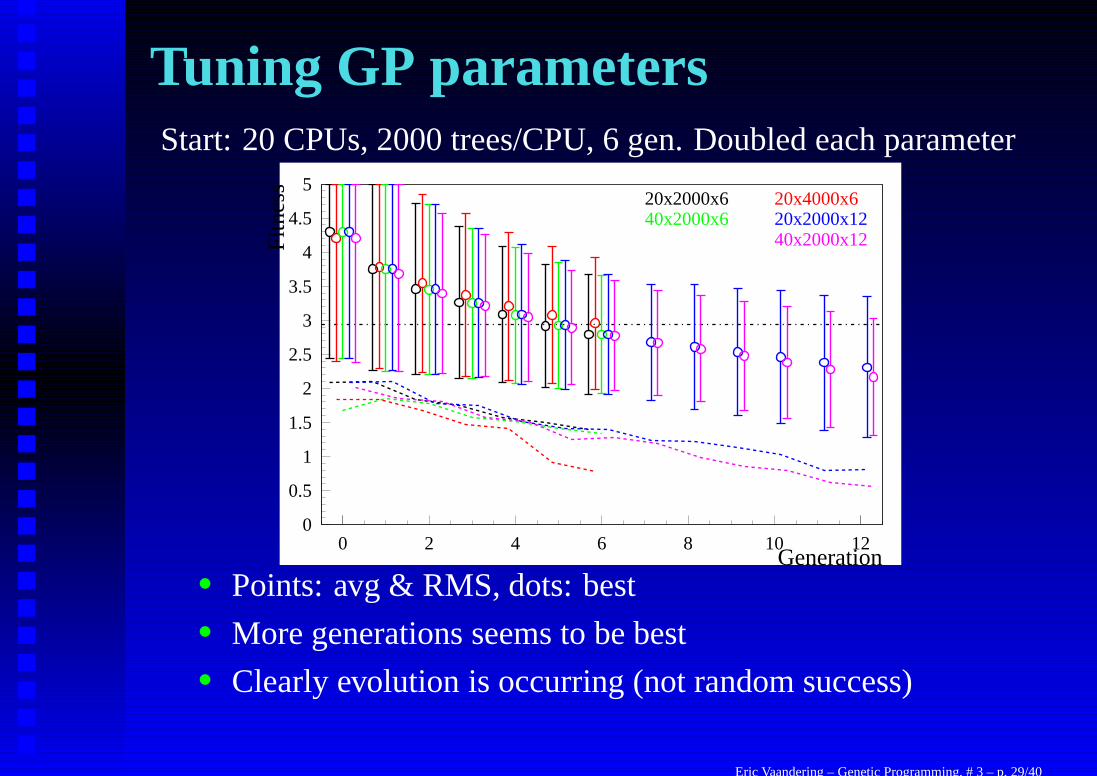
Tuning GP parametersStart: 20 CPUs, 2000 trees/CPU, 6 gen. Doubled each parameter
0
0.5
1
1.5
2
2.5
3
3.5
4
4.5
5
0 2 4 6 8 10 12Generation
Fitn
ess
20x2000x6 20x4000x640x2000x6 20x2000x12
40x2000x12
• Points: avg & RMS, dots: best• More generations seems to be best• Clearly evolution is occurring (not random success)
Eric Vaandering – Genetic Programming, # 3 – p. 29/40

D+ → K+π+π−
While Λ+c → pK+π− is the analysis we’re pursuing with this
method, D+ → K+π+π− is a useful check.
There is too much data to optimize on all of it, so we choose tooptimize just on 20% of the data.
This branching ratio has been measured and is surprisingly large(about 3 tan4 θc). The PDG value is 0.75 ± 0.16% relative toD+ → K−π+π+.
A FOCUS branching ratio measurement and Dalitz analysis isunderway with about 200 events in this mode.
Eric Vaandering – Genetic Programming, # 3 – p. 30/40
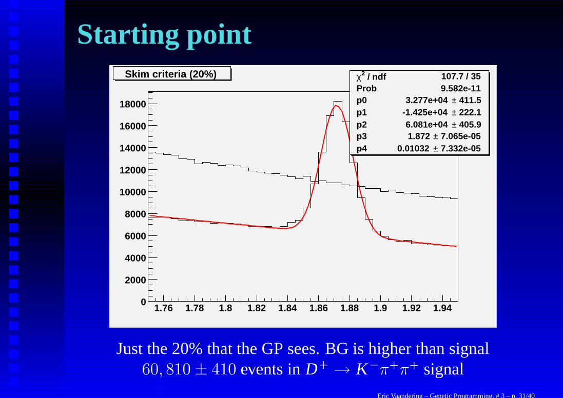
Starting point / ndf 2χ 107.7 / 35
Prob 9.582e-11p0 411.5± 3.277e+04 p1 222.1± -1.425e+04 p2 405.9± 6.081e+04 p3 7.065e-05± 1.872 p4 7.332e-05± 0.01032
1.76 1.78 1.8 1.82 1.84 1.86 1.88 1.9 1.92 1.940
2000
4000
6000
8000
10000
12000
14000
16000
18000
Skim criteria (20%) / ndf 2χ 107.7 / 35Prob 9.582e-11p0 411.5± 3.277e+04 p1 222.1± -1.425e+04 p2 405.9± 6.081e+04 p3 7.065e-05± 1.872 p4 7.332e-05± 0.01032
Skim criteria (20%) / ndf 2χ 107.7 / 35Prob 9.582e-11p0 411.5± 3.277e+04 p1 222.1± -1.425e+04 p2 405.9± 6.081e+04 p3 7.065e-05± 1.872 p4 7.332e-05± 0.01032
1.76 1.78 1.8 1.82 1.84 1.86 1.88 1.9 1.92 1.940
2000
4000
6000
8000
10000
12000
14000
16000
18000
/ ndf 2χ 107.7 / 35Prob 9.582e-11p0 411.5± 3.277e+04 p1 222.1± -1.425e+04 p2 405.9± 6.081e+04 p3 7.065e-05± 1.872 p4 7.332e-05± 0.01032
Skim criteria (20%)
Just the 20% that the GP sees. BG is higher than signal60, 810 ± 410 events in D + → K−π+π+ signal
Eric Vaandering – Genetic Programming, # 3 – p. 31/40
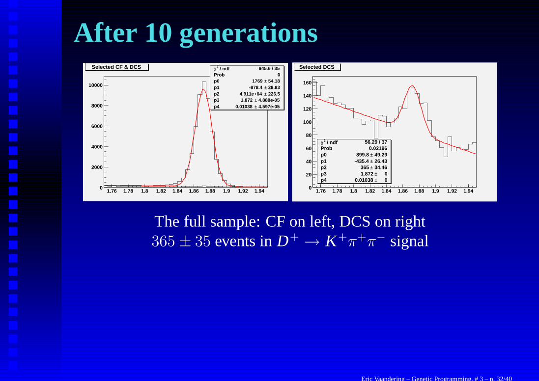
After 10 generations
1.76 1.78 1.8 1.82 1.84 1.86 1.88 1.9 1.92 1.940
2000
4000
6000
8000
10000
Selected CF & DCS / ndf 2χ 945.6 / 35Prob 0p0 54.18± 1769 p1 28.83± -878.4 p2 226.5± 4.911e+04 p3 4.888e-05± 1.872 p4 4.597e-05± 0.01038
Selected CF & DCS
/ ndf 2χ 56.29 / 37Prob 0.02196p0 49.29± 899.8 p1 26.43± -435.4 p2 34.46± 365 p3 0± 1.872 p4 0± 0.01038
1.76 1.78 1.8 1.82 1.84 1.86 1.88 1.9 1.92 1.940
20
40
60
80
100
120
140
160
/ ndf 2χ 56.29 / 37Prob 0.02196p0 49.29± 899.8 p1 26.43± -435.4 p2 34.46± 365 p3 0± 1.872 p4 0± 0.01038
Selected DCS
The full sample: CF on left, DCS on right365 ± 35 events in D+ → K+π+π− signal
Eric Vaandering – Genetic Programming, # 3 – p. 32/40

Data MC comparisonsSince these decays are nearly identical, what is important is thatthe efficiency of the tree for CF and DCS modes is the same.What need not be known is the absolute efficiency on a singlemode.
For the program which generated this, the MC efficiencies are:
CF Eff. (%) DCS Eff. (%)Skim cuts 6.99 ± 0.01 6.71 ± 0.01
GP Selection 1.12 ± 0.01 1.11 ± 0.01
GP/Skim 16.03 ± 0.08 16.58 ± 0.09
But, we can look at GP/Skim for the CF data.We find 16.15 ± 0.08%.
So, not only do the GP efficiencies for MC agree, the one placewe can compare the GP on MC and data, it also comes out right.
Good modeling is important if you need to understand the GP indetail.
Eric Vaandering – Genetic Programming, # 3 – p. 33/40
Data MC comparisonsSince these decays are nearly identical, what is important is thatthe efficiency of the tree for CF and DCS modes is the same.What need not be known is the absolute efficiency on a singlemode.
For the program which generated this, the MC efficiencies are:
CF Eff. (%) DCS Eff. (%)Skim cuts 6.99 ± 0.01 6.71 ± 0.01
GP Selection 1.12 ± 0.01 1.11 ± 0.01
GP/Skim 16.03 ± 0.08 16.58 ± 0.09
But, we can look at GP/Skim for the CF data.We find 16.15 ± 0.08%.
So, not only do the GP efficiencies for MC agree, the one placewe can compare the GP on MC and data, it also comes out right.
Good modeling is important if you need to understand the GP indetail. Eric Vaandering – Genetic Programming, # 3 – p. 33/40

10th generation resultsin
neg
<=>
/
σt `/σ`
<=>
min
OoT min
cos
ln
#τ
AND
<=>
min
OoT sign
Σp2T
POT
NOT
IF
f(n)
XOR
OSµ πcon
AND
xy
Iso2 OoT
<
KChi σt
<
cos
Iso1
>
∆πK 1 0
Eric Vaandering – Genetic Programming, # 3 – p. 34/40

ConclusionsThis method shows promise, but there are some caveats
• More challenging for modeling• Perhaps best used where statistical errors dominate• Trees are very complex and any attempt to understand the
whole thing may be pointless
However• Worthwhile to try to understand parts of trees• Combination CLP - Iso1 occurred often
• Now being used in other analyses• Even simpler trees do better than the cuts they suggest
We think this novel method at least deserves further exploration
Eric Vaandering – Genetic Programming, # 3 – p. 35/40
SW Mechanics & ConclusionsIs interfacing to an existing experiment’s code difficult?
• Genetic programming framework• C language based lilgp from MSU Garage group• Modified for parallel use (PVM) by Vanderbilt Med
Center group• Parallel version allows sub-population exchange
• Physics variables start with standard FOCUS analysis• Write HBOOK ntuples, convert to Root Trees• Write a little C++ code to access Trees, fill and fit
histograms (using MINUIT) and return the fitinformation to the lilgp framework
• This is actually pretty easy
Eric Vaandering – Genetic Programming, # 3 – p. 36/40

HomeworkOk, now for the not-so-fun part. I’m supposed to give you ahomework assignment. We’ll make it easy:
• On the “Resources” slide are several web pages withsoftware
• Look around and pick a software package in your favoritelanguage• C++, C, Java• Perl, Ruby, Python• FORTRAN?!?!, LISP, others
• Most or all of these will have example problems and code• Pick one you like, change the evolutionary parameters and
try changing the problem too
The idea is just to get your feet wet a little.
I also want to hear your impressions, because I’ve only used oneof these frameworks (lilgp).
Eric Vaandering – Genetic Programming, # 3 – p. 37/40

GA & GP ResourcesThere is a lot of information on the web about GeneticAlgorithms and Programming:
• http://www.aic.nrl.navy.mil/galist/ —Genetic Algorithms
• http://www.genetic-programming.org/ —John Koza
Software frameworks for both GA and GP exist in almost everylanguage (most have several)
• http://www.genetic-programming.com/coursemainpage.html#_Sources_of_Software
• http://zhar.net/gnu-linux/howto/ – GNU AIHowTo (GA/GP/Neural nets, etc.)
• http://www.grammatical-evolution.org —GA–GP Translator
Eric Vaandering – Genetic Programming, # 3 – p. 38/40

Backup slides
Backup slides
Eric Vaandering – Genetic Programming, # 3 – p. 39/40
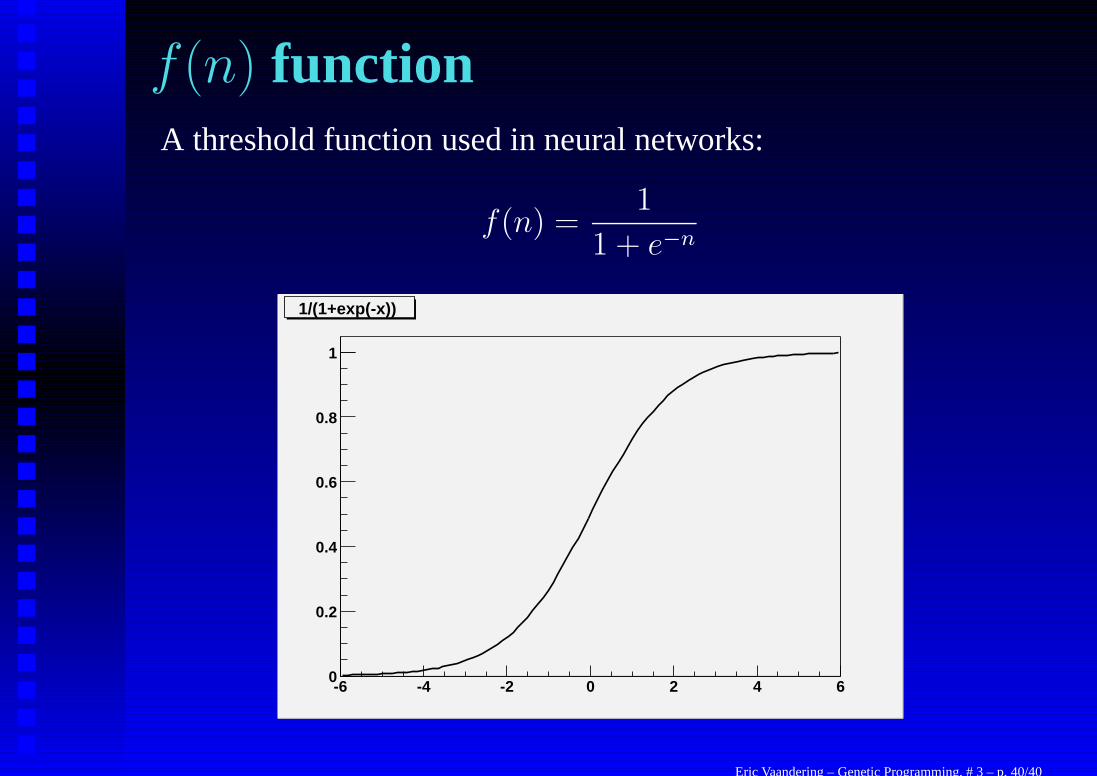
f (n) functionA threshold function used in neural networks:
f(n) =1
1 + e−n
-6 -4 -2 0 2 4 60
0.2
0.4
0.6
0.8
1
1/(1+exp(-x))
Eric Vaandering – Genetic Programming, # 3 – p. 40/40


![Notification of Delay Due to d 913-COR-ALT-ADM-000159[1]](https://cdn.vdocument.in/doc/165x107/55cf861f550346484b948228/notification-of-delay-due-to-d-913-cor-alt-adm-0001591.jpg)