ORI GIN AL PA PER
Genetic programming on graphics processing units
Denis Robilliard • Virginie Marion-Poty •
Cyril Fonlupt
Received: 24 November 2008 / Revised: 11 September 2009 / Published online: 14 October 2009
� Springer Science+Business Media, LLC 2009
Abstract The availability of low cost powerful parallel graphics cards has stim-
ulated the port of Genetic Programming (GP) on Graphics Processing Units (GPUs).
Our work focuses on the possibilities offered by Nvidia G80 GPUs when pro-
grammed in the CUDA language. In a first work we have showed that this setup
allows to develop fine grain parallelization schemes to evaluate several GP pro-
grams in parallel, while obtaining speedups for usual training sets and program
sizes. Here we present another parallelization scheme and optimizations about
program representation and use of GPU fast memory. This increases the compu-
tation speed about three times faster, up to 4 billion GP operations per second. The
code has been developed within the well known ECJ library and is open source.
Keywords Genetic algorithms � Genetic programming �Graphics processing units � Parallel processing
1 Introduction
It is well known that the most time consuming part of a Genetic Programming (GP)
run is the evaluation process. When dealing with complex real world problems like
those addressed by Koza et al. in their last book [1], thousands or even millions of
programs need to be evaluated at each generation. For instance, the rediscovery of
D. Robilliard (&) � V. Marion-Poty � C. Fonlupt
Univ. Lille Nord de France, ULCO, LIL, Maison de la Recherche Blaise Pascal,
50 rue Ferdinand Buisson, BP 719, 62228 CALAIS Cedex, France
e-mail: [email protected]
V. Marion-Poty
e-mail: [email protected]
C. Fonlupt
e-mail: [email protected]
123
Genet Program Evolvable Mach (2009) 10:447–471
DOI 10.1007/s10710-009-9092-3
previously patented inventions with the use of GP required a population of
10,000,000 programs. Even if the training set is limited (say some hundreds of
cases), this huge population size makes GP runs impractical on common systems.
Several schemes have been proposed in the literature to speed up GP. For
example: bypassing the evaluation of some of the evolved programs [2, 3]; caching
common subtrees to accelerate the overall evaluation process [4]; using a divide and
conquer strategy in order to minimize the computational cost [5]; devising dedicated
crossovers to reduce the bloat [6] and thus the evaluation cost; or evolving programs
directly in machine code [7, 8]. Another common strategy is to parallelize or
distribute GP computations, e.g. [9–12]. This parallelization or distribution of GP is
an efficient answer to the evaluation bottleneck, but it has the drawback that parallel
or distributed systems are not always available and are often quite expensive.
Within the parallelization paradigm, newly introduced graphics processing units
(GPUs) provide fast parallel hardware for a fraction of the cost of a traditional
parallel system. GPUs are designed to efficiently compute graphics primitives in
parallel to produce pixels for the video screen. Driven by ever increasing
requirements from the video game industry, recent GPUs are very powerful and
flexible processors, while their price remains in the range of mass consumer market.
They now offer floating-point calculation much faster than today’s CPU and,
beyond graphics applications, they are able to address general problems that can be
expressed mainly as data-parallel computations, i.e. the same code is executed on
many different data.
Several general purpose high level-languages for GPUs have become available
such as Brook,1 Sh2 (now stopped as an open source package but continued as a
commercial platform under the name RapidMind), Accelerator from Microsoft
Research, or PeakStream. Thus developers do not need any more to master the extra
complexity of graphics programming APIs when they design non graphics
applications on GPUs.3 With the G80 family GPUs, Nvidia proposes the CUDA
development kit (Compute Unified Device Architecture) that is based on a C-like
general purpose language, allowing fine control over the hardware capabilities.
Exploiting the power of GPUs within the framework of evolutionary computation
has been done first for genetic algorithms, e.g. [13–18]. Then implementation
schemes of Genetic Programming on GPU have been recently released, based either
on dynamic compilation of GP individuals [19–21] or on interpretation of the GP
programs [22, 23]. Some GP application papers that take advantage of GPU power
have already been issued [24–26] (see also the General Purpose Genetic
Programming on GPU site).4
In [19–21], Harding et al. and Chitty have obtained interesting speedups but
mainly for large individuals and/or several thousands fitness cases. In [19] this was
acknowledged as a weakness of this scheme: ‘‘Many typical GP problems do not
1 http://www.graphics.stanford.edu/projects/brookgpu/.2 http://www.libsh.org/.3 See http://www.gpgpu.org for a survey.4 http://www.gpgpgpu.com.
448 Genet Program Evolvable Mach (2009) 10:447–471
123
have large sets of fitness cases...’’ and ‘‘this leads to a gap between what we can
realistically evaluate, and what we can evolve’’. We also think that being able to
speed up evolution of programs against a moderate number of fitness cases is useful
in many of today’s GP problems. For example, GP is often used to perform
supervised classification, where it may be difficult to provide large sets of labeled
training cases, especially when labeling requires human intervention as in medical
diagnosis.
In order to exploit the power of the GPU on small training sets size, we proposed
in [23] a parallelization scheme based on interpretation rather than compilation of
GP programs. In this previous paper we explored the possibilities offered by the
Nvidia G80 GPU and its successors, organized around a Single Program Multiple
Data (SPMD) architecture, rather than Single Instruction Multiple Data (SIMD).
Our algorithm allowed one to evaluate simultaneously several different GP
individuals in parallel, delivering speedups for small training sets and as a
consequence leaving more computational power available to increase the population
size of the GP system. Another interpreter-based approach, implemented with a high
level GPU toolkit, was proposed independently by Langdon and Banzhaf in [22],
but, since both papers were written independently, no comparison was done.
Moreover the actual distribution of the computational load on the GPU in [22] is
unknown since it is masked by the RapidMind high level toolkit.
This new paper focusses on filling this gap: i.e. measuring the improvements
brought by our SPMD parallelization scheme. In order to achieve this goal, we
implement another algorithm that relies on a simpler, more intuitive, SIMD inspired
parallel scheme, that may be close to those automatically implemented by high level
GPU toolkits.
This comparative study allows us:
– to validate our previous work versus the simpler SIMD scheme and compare
their behavior on different problems, population and training set sizes; this is
important since that SIMD scheme is the natural solution that comes to mind
when considering parallelization of GP, and we suspect it is the scheme used by
high level GPU programming toolkit when doing automatic parallelization;
– to report absolute speed measurements that allow comparison with Langdon and
Banzhaf’s experiments published in [22];
– to provide more refined guidelines for GP implementation on GPU, notably
about load balancing (notably minimal number of blocks see Sect. 5) and on-
chip high-speed shared memory;
– to promote the use and/or development of SPMD-aware programming toolkits,
as the speed gains are mostly dependent on this feature.
In this paper, we first recall the parallel scheme we proposed in [23], and we then
define another parallel scheme that exploits the G80 as a standard SIMD device.
We compare the computational speed of both schemes for different types of
benchmarks. These experiments support the need for an explicit management of
computations in order to benefit from the SPMD characteristic. Further enhance-
ments are implemented and evaluated: changing the representation of GP programs
in the evolutionary engine and caching them in fast memory for evaluation on GPU.
Genet Program Evolvable Mach (2009) 10:447–471 449
123
We then test this final scheme on a benchmark taken from [22] in order to compare
it with another existing GPU implementation.
To implement these algorithms, we use the popular ECJ library [27] and we rely
on the Nvidia CUDA software development kit for evaluation on GPU since it
supports explicit low level distribution of computations. Higher level GPU toolkits,
while providing more comfort to the developer and more portability to the programs,
may hide critical parts of the system incurring severe losses in performance.
Note that even if the algorithms in this paper are primarily targeted for Nvidia
GPU graphic cards, it should be possible to port them onto ATI graphic hardware, as
both ATI and Nvidia new graphic cards share quite similar architectures. For
instance, in the case of the R600 graphics processing unit from ATI, each SIMD
array of 80 stream processors has its own sequencer and arbiter and so is close to the
multiprocessor concept implemented by Nvidia.
The rest of the paper is organized in the following way: the next section presents
the basic traits of the G80 GPU family and the CUDA programming language. In
Section 3 we present our two different parallelization schemes. Section 4 discusses
general issues about implementation and presents our set of benchmark problems. In
Section 5 we evaluate the gains brought by an SPMD-conscious implementation of
the GP evaluation phase. Section 6 introduces representation and memory
optimizations and gives final benchmark results. In Section 7 we present our
conclusions and discuss future issues.
2 G80 GPU architecture and CUDA language
From their origins, GPUs are dedicated graphics hardware organized as a pipeline
that manipulates very efficiently and very quickly graphics primitive operations.
Basically, this pipeline can be split into two main stages: the first stage is in charge
of manipulating 3D vertices on which transformations are applied (like rotation,
homothecy, etc.). The second stage implements operations on pixels that rely on
textures and colors. In previous generations of GPU, the first stage was performed
by so-called vertex processors while the second stage operations were done by
fragment processors also known as fragment shaders. Recent graphics cards are
based on a unified architecture where a pool of elementary processors can be used
either for first or second stage operations.
2.1 G80 architecture
The graphics card we consider is a Nvidia GeForce 8800 GTX based on the G80
GPU. It is natively limited to single precision floating point (32-bit data precision),
although double precision can be used through a software library. This hardware is
based on a unified architecture managed as a pool of 16 so-called multiprocessors.
A multiprocessor contains 8 elementary stream processors that operate at 1.35
GHz clock rate, giving a total number of 128 stream processors on the graphics card.
A multiprocessor also owns 16 KB of fast memory that can be shared by its 8 stream
processors, 8 KB of texture and constant cache and an independent program counter.
450 Genet Program Evolvable Mach (2009) 10:447–471
123
Multiprocessors are SIMD devices, meaning their inner 8 stream processors
execute the same instruction at every time step. Nonetheless alternative and loop
structures can be implemented: for example in case of an if instruction where some
of the stream processors must follow the then path while the others follow the
else path, both execution paths are serialized and stream processors not concerned
by an instruction are simply put into an idle mode. Putting some stream processors
in an idle mode to allow control structures is called divergence, and of course this
causes a loss of efficiency.
At the level of multiprocessors the G80 GPU works in SPMD mode (Single
Program, Multiple Data): every multiprocessor must run the same program, but they
do not need to execute the same instruction at the same time step (as opposed to
their internal stream processors), because each of them owns its private program
counter. So there is no divergence between multiprocessors.
2.2 Execution model
The execution model supported by the architecture and CUDA language relies on 3
concepts:
– A grid is a set of computations performed with a given kernel (a program
executed on the CPU).
– A grid is divided into blocks, each block is a subset of computations being
executed on a given multiprocessor. If there are enough multiprocessors all the
blocks of a grid are executed in parallel, otherwise a scheduler manages them
and their order of execution is not known in advance. A block cannot access the
fast memory bank or registers of another block.
– A block is itself divided into threads that are scheduled on the elementary
stream processors of the multiprocessor that runs the block. The order of
execution of threads is not known in advance. On the G80, the number of
threads is a multiple of 32, thus there are always more threads than stream
processors in a multiprocessor. This scheduling allows the amortization of
memory access delays.
A thread can be roughly viewed as the smallest elementary computation process
on the parallel device.
2.3 CUDA language overview
CUDA is an extension of the C language, it is free software although proprietary
to Nvidia. Several general purpose libraries are available for CUDA, such as
linear algebra, FFT, etc.5 Its main drawback is that it runs only on Nvidia
hardware from the G80 and up, but it offers fine grain access to the architecture.
As usual for GPU software toolkits, programs are divided in two parts, one runs
5 see http://www.nvidia.com/object/cuda_home.html.
Genet Program Evolvable Mach (2009) 10:447–471 451
123
on the host CPU and the other on the GPU device, this part of code being called
the kernel in the CUDA jargon. The host code is generally responsible for
transferring data and loading the kernel code to the graphics card memory,
performing input and output (with the obvious exception of the graphics display),
and calling the kernel code.
Inside a CUDA thread, the program can request the block and thread identifiers
(these are sequential integers) and then choose to execute some task depending on
this information, i.e. this allows one to associate tasks to given blocks or threads.
We make a heavy use of this ability in Sect. 3.2, to reduce divergence between
multiprocessors by carefully assigning tasks on blocks. To the best of our
knowledge, this management of threads is only available with CUDA.
By default the execution order of threads is decided by the scheduler, so the
language provides a syncthread instruction that synchronizes threads of a block,
thus the programmer can insure that a given set of operations are done before
proceeding further. It is also possible to declare variable and arrays allocated either
in the fast 16 KB memory bank of each multiprocessor (4 clock cycles access
overhead) or in the global memory of the graphics card although it is much more
slower (up to 600 clock cycles latency overhead, at least for the first memory word
of a sequence of consecutive addresses). Besides its large capacity (760 MB on the
Nvidia 8800 GTX card) global memory has also the advantage that it is accessible
from every thread running on the GPU, thus allowing complex operations.
Furthermore global memory can also be cached. Notice that neither recursion nor
function pointers are yet available on GPU processors, thus these concepts are
missing in the language. Pointers to data (variable, arrays) are available.
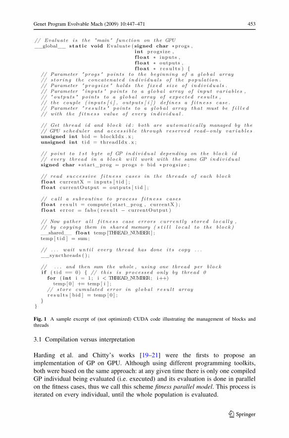
We provide an excerpt of CUDA code (not optimized), in a context similar to GP
regression, to illustrate how one can distribute the load on specific blocks and
threads, i.e. this can be done simply by testing and using the numerical identifier of
threads and blocks, somewhat close to programming multi-threaded applications
with fork instructions. We assume our sample application spawned as many blocks
as GP programs and as many threads as fitness cases. Then every block of threads is
supposed to process its own GP individual, the threads evaluating the different
fitness cases. When browsing the code displayed in Fig. 1, the reader should keep in
mind that the instructions will be performed in parallel by all the threads and that
local variables are local to threads. We hope it shows that using the parallelism of
GPU is not as complicated as it is sometimes rumored.
3 Population parallel models
Modern graphic cards including the G80 family are either SPMD or SIMD devices.
Several parallel models are possible depending on the hardware capabilities,
software development kit and, of course, programmer’s choice. First we discuss GP
program compilation versus interpretation issues. Then we recall the so-called
BlockGP parallel model that we introduced in [23], and we detail another parallel
model, called ThreadGP. Both these schemes use an interpreter to evaluate
simultaneously several individuals from a given generation.
452 Genet Program Evolvable Mach (2009) 10:447–471
123
3.1 Compilation versus interpretation
Harding et al. and Chitty’s works [19–21] were the firsts to propose an
implementation of GP on GPU. Although using different programming toolkits,
both were based on the same approach: at any given time there is only one compiled
GP individual being evaluated (i.e. executed) and its evaluation is done in parallel
on the fitness cases, thus we call this scheme fitness parallel model. This process is
iterated on every individual, until the whole population is evaluated.
Fig. 1 A sample excerpt of (not optimized) CUDA code illustrating the management of blocks andthreads
Genet Program Evolvable Mach (2009) 10:447–471 453
123
Of course, as the G80 is an SPMD device we cannot perform the direct execution
of several different GP programs in parallel. However, emulating MIMD tasks on a
basically SIMD hardware can be done in the form on an interpreter that considers
the set of programs as data (see e.g. [28]). This solution was chosen by Juille and
Pollack when they parallelized GP on the MASPAR machine [10], evaluating
several different programs simultaneously. We call this approach populationparallel model, and in [23] we showed that this scheme yields speedups even for a
small number of fitness cases and short programs. The same approach was proposed
successfully by Langdon and Banzhaf in [22].
Compilation versus interpretation is clearly a trade-off choice: the cost of
iterating interpreted code on the training cases is to be balanced against the
compilation overhead and reduced cost of iterating compiled instructions. If there
are few training cases, meaning few iterations, then the interpreter may be a sensible
solution.
Moreover, if we execute one GP program at a time (either compiled or
interpreted), then we parallelize only the training data, and we might well have not
enough data to fill all the ALU pipelines of the elementary stream processors. This
would leave the GPU under-exploited, especially since new generation GPUs have
several hundreds of elementary processors. On the contrary interpreting several
programs in parallel increases the computation load. For all these reasons we chose
an interpreter scheme in this work, the implementation details being given in
Sect. 4.
3.2 BlockGP scheme
In order to limit the occurrences of divergence, we proposed in [23] to dispatch the
population of GP trees in such a way that, at any time, each multiprocessor
interprets only one GP tree. That is, GP trees are parallelized at the level of
multiprocessors, thus allowing up to 16 GP programs to be interpreted in parallel on
the G80. The fitness computation of a given tree is in turn parallelized on the 32
threads running on the multiprocessor that are scheduled on its 8 stream processors.
This scheme is illustrated in Fig. 2. So every stream processor evaluates around 1/
8th of the training cases (variations may occur due to scheduling). This 1/8th factor
should leave enough data to fill the ALU pipelines in most cases, even with small
training sets.
To highlight the main characteristics of the BlockGP scheme:
– Every GP program is interpreted by all threads running on a given
multiprocessor.
– The number of fitness cases to be processed by each thread is greater than in a
fitness parallel scheme (as defined in Sect. 3.1), thus BlockGP is more
computationally intensive, provided the population size is at least as big as the
number of multiprocessors (which is most often the case on current GPU).
– There is no divergence due to differences between GP programs, since
multiprocessors are independent.
454 Genet Program Evolvable Mach (2009) 10:447–471
123
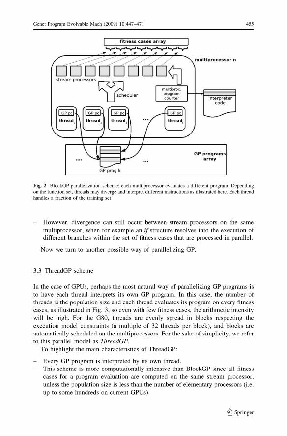
– However, divergence can still occur between stream processors on the same
multiprocessor, when for example an if structure resolves into the execution of
different branches within the set of fitness cases that are processed in parallel.
Now we turn to another possible way of parallelizing GP.
3.3 ThreadGP scheme
In the case of GPUs, perhaps the most natural way of parallelizing GP programs is
to have each thread interprets its own GP program. In this case, the number of
threads is the population size and each thread evaluates its program on every fitness
cases, as illustrated in Fig. 3, so even with few fitness cases, the arithmetic intensity
will be high. For the G80, threads are evenly spread in blocks respecting the
execution model constraints (a multiple of 32 threads per block), and blocks are
automatically scheduled on the multiprocessors. For the sake of simplicity, we refer
to this parallel model as ThreadGP.
To highlight the main characteristics of ThreadGP:
– Every GP program is interpreted by its own thread.
– This scheme is more computationally intensive than BlockGP since all fitness
cases for a program evaluation are computed on the same stream processor,
unless the population size is less than the number of elementary processors (i.e.
up to some hundreds on current GPUs).
Fig. 2 BlockGP parallelization scheme: each multiprocessor evaluates a different program. Dependingon the function set, threads may diverge and interpret different instructions as illustrated here. Each threadhandles a fraction of the training set
Genet Program Evolvable Mach (2009) 10:447–471 455
123
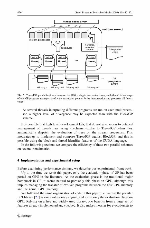
– As several threads interpreting different programs are run on each multiproces-
sor, a higher level of divergence may be expected than with the BlockGP
scheme.
It is possible that high level development kits, that do not give access to detailed
management of threads, are using a scheme similar to ThreadGP when they
automatically dispatch the evaluation of trees on the stream processors. This
motivates us to implement and compare ThreadGP against BlockGP, and this is
possible using the block and thread identifier features of the CUDA language.
In the following sections we compare the efficiency of these two parallel schemes
on several benchmarks.
4 Implementation and experimental setup
Before examining performance timings, we describe our experimental framework.
Up to the time we write this paper, only the evaluation phase of GP has been
ported on GPU in the literature. As the evaluation phase is the traditional major
bottleneck in GP, it seems natural to port only this phase on GPU, although this
implies managing the transfer of evolved programs between the host CPU memory
and the kernel GPU memory.
We followed the same organization of code in this paper, i.e. we use the popular
ECJ library [27] as our evolutionary engine, and move only the evaluation phase on
GPU. Relying on a free and widely used library, one benefits from a large set of
features already implemented and checked. It also makes it easier for evolutionists to
Fig. 3 ThreadGP parallelization scheme on the G80: a single interpreter is run; each thread is in chargeof one GP program, manages a software instruction pointer for its interpretation and processes all fitnesscases
456 Genet Program Evolvable Mach (2009) 10:447–471
123

run experiments on GPU: they just have to write the fitness function code in CUDA,
following the example code we provide on our web site [29]. They can even keep a
custom representation already written for ECJ, although in this case they will need to
provide a method for translating programs in order to merge their code with ours.
Anyway it would not be easy to implement a complete GP system on current
GPUs because neither recursion nor function pointers are yet available on these
processors. These two programming language features are not mandatory, but their
absence would result in a more obfuscated and less flexible code, for example when
dealing with pointed representations such as pointed trees or graphs. Current GP
libraries also heavily rely on genericity, which would be challenging to implement
without function pointers. For these reasons we think it is unlikely to see the release
of general purpose GP systems with breeding implemented on current GPUs,
although limited systems are possible to implement.
4.1 Bridging the ECJ library and the CUDA-written interpreter
The ECJ library is written in the Java language and it offers a set of already
implemented standard benchmarks, that we use to obtain the reference CPU timings
in Sect. 6.2. We need to transfer GP solutions and fitness cases from Java to CUDA,
which is done via the Java Native Interface (JNI).
In Sect. 5, our experiments are done with the mainstream tree representation for
GP individuals. This tree representation implies the use of hidden pointers, so GP
solutions are scattered into the Java Virtual Machine memory. Copying programs in
this representation to the graphics card would have implied a great number of small
data transfers which is overly costly. So we first translate GP trees in a linear
representation inspired by Reverse Polish Notation (RPN). Every program tree is
turned into as a sequence of operators and operands that are represented as floats so
that ephemeral random constants (ERCs) can be stored in-line. Programs are
concatenated into an array that also stores a table of pointers to the first instruction
of every program. Then the array is copied to the graphics card as a single chunk of
memory. Notice that we do not transfer individuals that are mere copies from the
previous generation, since they are already evaluated (this is known through the ECJ
‘‘evaluated’’ flag).
For the sake of efficiency, the if and iflte6 structures, and logical operators
and, or can be implemented as shortcut versions, i.e. branches that do not need to
be evaluated are bypassed. This is done by inserting jump opcodes, as in standard
code generation as in [30], and thus the resulting code interpreted on the GPU is not
true RPN since some operands are not evaluated.
For example, let us take the LISP-like expression:
ð� ðþ 3 1Þðiflte 3 4ð� 2 3Þ 5ÞÞThis expression is translated into the following linear program, where ifg means
‘‘if greater’’ and jumps conditionally to the corresponding label if the top of stack is
dominated by the previous value:
6 iflte is a quaternary operator that stands for: if sibling1 less than sibling2 then sibling3 else sibling4.
Genet Program Evolvable Mach (2009) 10:447–471 457
123
push3; push1; add; push3; push4; ifglabel1; push2; push3;
sub; jmplabel2; label1push5; label2mul;
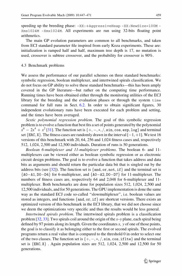
A stack-based interpreter is very easy to write for the execution of RPN-like
solutions. The interpreter code is run on the GPU and is composed of a main loop
fetching the next instruction to process, and a switch that performs the operations
required depending on the instruction, see pseudo-code in Table 1.
In a second set of experiments, detailed in Sect. 6, we directly use RPN notation
as the basic representation for GP trees, thus departing from the ECJ standard, while
retaining ECJ evolution engine.
4.2 Experimental setup
Our test machine is equipped with an Intel Core-2 6600 at 2,4 GHz CPU and 2
Gbytes RAM, and has two graphics card: an 8400GS dedicated to the display, and
the 8800GTX that is reserved for the computations and thus not attached to an X
server. This dual cards setting allows one to get cleaner timings (no interference
with the display). Note that it is possible to use the 8800GTX for both display and
GP evolution, although with constraints: during intensive computation, the user
interaction with the X desktop is suspended; moreover any given call to the GPU
(i.e. executing the interpreter in our case) cannot last more than 5 s, otherwise the
process is killed by the X server watchdog process.
For the parallel schemes we use the minimal number of 32 threads per
multiprocessor for all experiments. The ECJ code is run using the Sun JDK 1.6 with
1 Gbyte RAM reserved for the Java virtual machine and recommended flags for
Table 1 Pseudo code of the interpreter
sp = 0; // initialize stack pointer
while there is an instruction to process {
fetch instruction;
switch (instruction) {
case OPERAND : stack[sp??] = data; // push data onto stack
case ADD : stack[sp-2] = stack[sp-1] ? stack[sp-2]; sp-;
case MUL : stack[sp-2] = stack[sp-1] * stack[sp-2]; sp-;
case IFG : if (stack[sp-2][stack[sp-1]) then
fetch new instruction pointer value;
sp = sp-2;
endif
case JUMP : fetch new instruction pointer value;
. . .
}
}
458 Genet Program Evolvable Mach (2009) 10:447–471
123
speeding up the breeding phase: -XX:?AggressiveHeap -XX:NewSize=100M -
Xms1024M -Xmx1024M. All experiments are run using 32-bits floating point
arithmetics.
The main GP evolution parameters are common to all benchmarks, and taken
from ECJ standard parameter file inspired from early Koza experiments. These are:
initialization is ramped half and half, maximum tree depth is 17, no mutation is
used, crossover is subtree crossover, and the probability for crossover is 90%.
4.3 Benchmark problems
We assess the performance of our parallel schemes on three standard benchmarks:
symbolic regression, boolean multiplexer, and intertwined spirals classification. We
do not focus on GP ability to solve these standard benchmarks—this has been amply
covered in the GP literature—but rather on the computing time performance.
Running times have been obtained either through the monitoring utilities of the ECJ
library for the breeding and the evaluation phases or through the system time
command for full runs in Sect. 6.2. In order to obtain significant figures, 30
independent evolutionary runs have been executed for each problem and setting,
and the times have been averaged.
Sextic polynomial regression problem. The goal of this symbolic regression
problem is to evolve a function that best fits a set of points generated by the polynomial
x6 - 2x4 ? x2 [31]. The function set is fþ;�; �; =; sin; cos; exp; logg and terminal
set fERC; Xg. The fitness cases are randomly drawn in the interval [-1, ?1]. We test 16
versions of this benchmark with 20, 64, 256 and 1,024 fitness cases and, respectively
512, 1,024, 2,500 and 12,500 individuals. Duration of runs is 50 generations.
Boolean 6-multiplexer and 11-multiplexer problems. The boolean 6- and 11-
multiplexers can be viewed either as boolean symbolic regression or as electronic
circuit design problems. The goal is to evolve a function that takes address and data
bits as arguments and should return the particular data bit that is singled out by the
address bits (see [32]). The function set is fand; or; not; ifg and the terminal set is
fA0�A1; D0�D4g for 6-multiplexer, and fA0�A2; D0�D7g for 11-multiplexer. The
numbers of fitness cases are, respectively 64 and 2,048 for 6-multiplexer and 11-
multiplexer. Both benchmarks are done for population sizes 512, 1,024, 2,500 and
12,500 individuals, and for 50 generations. The GPU implementation is done the same
way as the standard ECJ code so-called ‘‘slowmultiplexer’’, i.e. boolean values are
stored as integers, and functions fand; or; ifg are shortcut versions. There exists an
optimized version of this benchmark in the ECJ library, that we did not choose since
we deem the optimizations very specific and thus the results would be less general.
Intertwined spirals problem. The intertwined spirals problem is a classification
problem [32, 33]. Two spirals coil around the origin of the x–y plane, each spiral being
defined by 97 points along its length. Given the coordinates x, y of one of those points,
the goal is to classify it as belonging either to the first or second spirals. The evolved
programs return a real value that is compared to the threshold 0 in order to select one
of the two classes. The function set is fþ;�; �; =; sin; cos; iflteg and the terminal
set is fERC; Xg . Again population sizes are 512, 1,024, 2,500 and 12,500 for 50
generations.
Genet Program Evolvable Mach (2009) 10:447–471 459
123
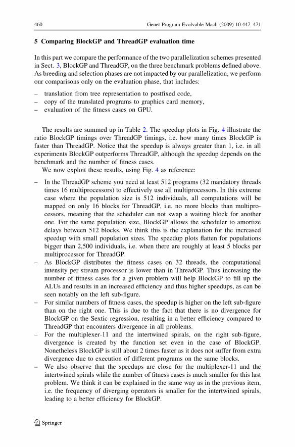
5 Comparing BlockGP and ThreadGP evaluation time
In this part we compare the performance of the two parallelization schemes presented
in Sect. 3, BlockGP and ThreadGP, on the three benchmark problems defined above.
As breeding and selection phases are not impacted by our parallelization, we perform
our comparisons only on the evaluation phase, that includes:
– translation from tree representation to postfixed code,
– copy of the translated programs to graphics card memory,
– evaluation of the fitness cases on GPU.
The results are summed up in Table 2. The speedup plots in Fig. 4 illustrate the
ratio BlockGP timings over ThreadGP timings, i.e. how many times BlockGP is
faster than ThreadGP. Notice that the speedup is always greater than 1, i.e. in all
experiments BlockGP outperforms ThreadGP, although the speedup depends on the
benchmark and the number of fitness cases.
We now exploit these results, using Fig. 4 as reference:
– In the ThreadGP scheme you need at least 512 programs (32 mandatory threads
times 16 multiprocessors) to effectively use all multiprocessors. In this extreme
case where the population size is 512 individuals, all computations will be
mapped on only 16 blocks for ThreadGP, i.e. no more blocks than multipro-
cessors, meaning that the scheduler can not swap a waiting block for another
one. For the same population size, BlockGP allows the scheduler to amortize
delays between 512 blocks. We think this is the explanation for the increased
speedup with small population sizes. The speedup plots flatten for populations
bigger than 2,500 individuals, i.e. when there are roughly at least 5 blocks per
multiprocessor for ThreadGP.
– As BlockGP distributes the fitness cases on 32 threads, the computational
intensity per stream processor is lower than in ThreadGP. Thus increasing the
number of fitness cases for a given problem will help BlockGP to fill up the
ALUs and results in an increased efficiency and thus higher speedups, as can be
seen notably on the left sub-figure.
– For similar numbers of fitness cases, the speedup is higher on the left sub-figure
than on the right one. This is due to the fact that there is no divergence for
BlockGP on the Sextic regression, resulting in a better efficiency compared to
ThreadGP that encounters divergence in all problems.
– For the multiplexer-11 and the intertwined spirals, on the right sub-figure,
divergence is created by the function set even in the case of BlockGP.
Nonetheless BlockGP is still about 2 times faster as it does not suffer from extra
divergence due to execution of different programs on the same blocks.
– We also observe that the speedups are close for the multiplexer-11 and the
intertwined spirals while the number of fitness cases is much smaller for this last
problem. We think it can be explained in the same way as in the previous item,
i.e. the frequency of diverging operators is smaller for the intertwined spirals,
leading to a better efficiency for BlockGP.
460 Genet Program Evolvable Mach (2009) 10:447–471
123
– A particular case is the multiplexer-6, that cumulates both a small number of
fitness cases and a high frequency of diverging operators: for this benchmark
BlockGP and ThreadGP exhibit comparable results. We recall that we observed
in [23] that the GPU was not faster than the CPU on this problem.
We do not report here the mean size of evolved trees, it can be found in the next
section Table 3: we recall that the trees are the same for both schemes, and since we
Table 2 Evaluation time in seconds for runs with one individual per block (BGP) and runs with one
individual per thread (TGP)
Problem Population size
# Cases: 512 1,024 2,500 12,500
Sextic 20
Time BGP 0.22 ± 0.08 0.40 ± 0.09 0.84 ± 0.20 4.26 ± 0.97
Time TGP 0.58 ± 0.26 0.79 ± 0.18 1.34 ± 0.34 6.08 ± 1.39
Speedup 2.45 ± 0.74 1.99 ± 0.10 1.60 ± 0.04 1.43 ± 0.02
Sextic 64
Time BGP 0.31 ± 0.13 0.44 ± 0.15 1.03 ± 0.36 5.55 ± 1.35
Time TGP 1.30 ± 0.42 1.64 ± 0.52 2.38 ± 0.62 12.10 ± 3.29
Speedup 4.36 ± 1.03 3.74 ± 0.93 2.52 ± 1.01 2.22 ± 0.50
Sextic 256
Time BGP 0.56 ± 0.20 0.89 ± 0.30 1.92 ± 0.72 10.54 ± 2.00
Time TGP 4.67 ± 2.19 6.52 ± 2.12 7.14 ± 0.62 33.77 ± 8.47
Speedup 8.28 ± 2.56 7.71 ± 2.70 3.92 ± 0.96 3.23 ± 0.74
Sextic 1024
Time BGP 1.10 ± 0.53 2.30 ± 0.87 6.15 ± 2.22 29.92 ± 7.91
Time TGP 14.47 ± 7.27 19.33 ± 6.82 29.97 ± 10.85 121.86 ± 30.21
Speedup 12.94 ± 3.29 8.59 ± 1.31 5.13 ± 1.61 4.20 ± 0.90
6-mult. 64
Time BGP 0.33 ± 0.10 0.57 ± 0.18 1.38 ± 0.32 6.29 ± 1.00
Time TGP 0.64 ± 0.18 0.85 ± 0.25 1.61 ± 0.37 6.96 ± 1.11
Speedup 1.92 ± 0.20 1.49 ± 0.09 1.17 ± 0.03 1.11 ± 0.02
11-mult. 2048
Time BGP 1.84 ± 0.69 2.87 ± 1.06 6.23 ± 2.22 29.20 ± 6.23
Time TGP 12.56 ± 4.08 11.85 ± 4.29 14.52 ± 4.87 62.85 ± 15.94
Speedup 6.95 ± 0.98 4.15 ± 0.43 2.34 ± 0.11 2.14 ± 0.12
Spirals 194
Time BGP 1.21 ± 0.48 2.32 ± 0.57 6.49 ± 2.28 33.54 ± 11.01
Time TGP 6.64 ± 2.23 7.93 ± 1.68 12.26 ± 3.91 61.37 ± 19.02
Speedup 5.67 ± 1.11 3.48 ± 0.55 1.92 ± 0.28 1.85 ± 0.21
Times and speedup BGP over TGP are given as mean and standard deviation over 30 runs, best timings
are in boldface
Genet Program Evolvable Mach (2009) 10:447–471 461
123

use shortcuts for the and, or, if and iflte operators, the evaluation time can not be
directly related to the mean tree size.
From these results, we select BlockGP as our base parallel scheme for the rest of
the paper.
6 Generic optimizations and final results
Increasing speed being the purpose of porting GP on GPU, we now introduce
representation and memory optimizations that are needed to fully exploit our
BlockGP algorithm. Then we present the final speed results in terms of the number
of GP operations per second, a measure introduced by Langdon and Banzhaf in [22].
6.1 GPU and CPU optimizations
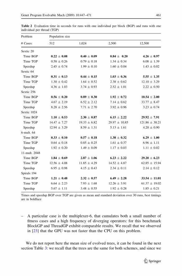
Removing tree to postfixed translation. In [23] we noticed that the reduction in
evaluation time for some problems is such that the breeding time is no longer
negligible. This is highlighted in Table 3 where breeding for standard ECJ trees and
evaluation are gathered for all our benchmarks. We can see that the ratio breeding
over evaluation time never drops below one third, and is often greater than one
meaning that in those case the breeding dominates the cost of the evaluation. We
can also notice that the lower ratios are associated to the benchmarks with:
– the more numerous fitness cases, such as sextic-1,024 versus other sextic
settings and multiplexer-11 versus multiplexer-6, since obviously evaluation
takes more time with more fitness cases,
– the smallest population sizes for a given number of fitness cases: we attribute
this to the degradation of the Java virtual machine performance when managing
huge number of objects, and also to fixed overheads when accessing the graphics
card for evaluation.
Mean Speedup BlockGP vs ThreadGP models
Sextic regression Problem
population size
spee
dup
fact
or
512 2500 12500
10
speedup=1(i.e. no speedup)
20 training cases64 training cases256 training cases1024 training cases
Mean Speedup BlockGP vs ThreadGP models
Multiplexer and Spirals
population size
spee
dup
fact
or
512 2500 12500
02
46
8
02
46
810
speedup=1(i.e. no speedup)
Multiplexer−6Multiplexer−11Intertwined Spirals
Fig. 4 BlockGP versus ThreadGP speedup for the evaluation phase. On the left, speedup on sexticregression x6 - 2x4 ? x2, on the right speedup on 6-multiplexer, 11-multiplexer and intertwined spirals(64, 2,048 and 194 training cases, respectively)
462 Genet Program Evolvable Mach (2009) 10:447–471
123
This confirms our previous claim that the breeding phase might no more be
considered negligible for common population sizes and fitness case numbers. Of
course this claim is dependent from our breeding implementation:
Table 3 Timings in seconds for breeding standard ECJ trees (on CPU) and evaluating them (on GPU)
with the BlockGP scheme
Problem Population size
# Cases: 512 1,024 2,500 12,500
Sextic 20
Breeding 0.48 0.91 2.26 23.65
Evaluation 0.22 0.40 0.84 4.26
Ratio 2.11 2.29 2.70 5.55
Tree size 48.28 60.93 62.86 64.68
Sextic 64
Breeding 0.54 0.82 2.28 24.54
Evaluation 0.31 0.44 1.03 5.55
Ratio 1.72 1.84 2.21 4.43
Tree size 51.16 54.53 61.72 66.24
Sextic 256
Breeding 0.52 0.87 2.12 24.20
Evaluation 0.56 0.89 1.92 10.54
Ratio 0.93 0.98 1.10 2.29
Tree size 50.38 60.83 58.36 65.72
Sextic 1024
Breeding 0.37 0.77 2.41 23.16
Evaluation 1.10 2.30 6.15 29.92
Ratio 0.34 0.34 0.39 0.77
Tree size 48.17 54.67 63.99 63.36
6-mult. 64
Breeding 0.96 1.75 5.71 48.71
Evaluation 0.33 0.57 1.38 6.29
Ratio 2.90 3.05 4.15 7.75
Tree size 138.72 127.49 132.09 120.60
11-mult. 2048
Breeding 1.05 2.07 7.00 66.11
Evaluation 1.84 2.87 6.23 29.20
Ratio 0.57 0.72 1.12 2.26
Tree size 160.03 151.76 149.69 156.24
Spirals 194
Breeding 1.08 2.31 10.89 88.28
Evaluation 1.21 2.32 6.49 33.54
Ratio 0.90 0.99 1.68 2.63
Tree size 161.92 167.49 196.46 197.00
Tree size, timings and the ratio breeding over evaluation timings are given as mean values over 30 runs
Genet Program Evolvable Mach (2009) 10:447–471 463
123
– it is done on the CPU,
– it is coded in Java,
– it uses the standard ECJ tree representation.
Porting the breeding on GPU is certainly an interesting option for future studies.
Here we have chosen to keep part of the advantages and flexibility of ECJ in order
to achieve sensible reduction in breeding time on the CPU via a change in the
representation of individuals. Thus, we aim to obtain competitive results for full run,
and not only the evaluation phase.
One obvious improvement is to modify the ECJ evolution engine in order not to
work with standard pointer-based trees but rather to directly manipulate and evolve
linear coded RPN trees. Doing this we do not need translation anymore before
copying the population to graphics card memory, although we still need to add
shortcut jumps if present. We also greatly decrease the number of object creations
and deletions which are time costly. It is rather easy to locate any subtree in a RPN
tree by parsing it and counting the number of expected arguments associated to each
node, along the lines proposed by W. B. Langdon in [34]. Thus crossover and
mutation operators can be written efficiently for linear arrays of RPN instructions.
In this scheme an individual is stored as a byte array, each byte coding an
operator or an operand. It is not convenient to store floating point ERCs inside the
individual array, so we choose to store a set of predefined ERCs that are associated
with predefined operands. A similar representation was used for linear genetic
programming by Brameier and Banzhaf [35], and also by Langdon in [34]. Notice
that this representation forces one to define a maximum length for individuals, or
else the insertion of mutated inner subtrees would shift arbitrary large array slices
and thus would downgrade performance. It obviously creates some incompatibilities
with the rest of ECJ code, nonetheless it still uses the standard breeding pipeline,
and the overall evolutionary framework.
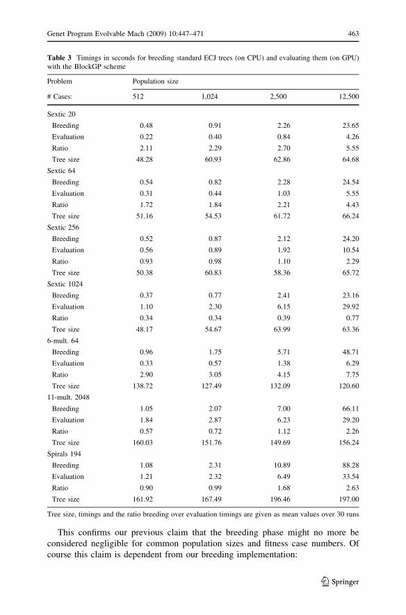
In Table 4 we illustrate the time savings brought by this breeding scheme for the
largest population size (12,500 individuals) where breeding is the more costly. Only
one setting as been reported for the sextic regression since the mean tree size and
thus the breeding time is very similar for all sextic settings. Breeding time and mean
Table 4 Comparison of breeding time in seconds between standard ECJ tree representation and RPN
representation for a population size of 12,500 individuals
Breeding scheme Sextic 1024 Multiplexer Intertwined spirals
6-bits 11-bits
Standard tree
Time 23.16 48.71 66.11 88.28
Size 63.36 120.60 156.24 197.00
RPN tree
Time 3.28 6.98 8.04 8.66
Size 67.22 120.60 156.24 163.68
Max. size 256 768 768 768
Time and mean tree size are averaged for 30 runs, best timings are in boldface
464 Genet Program Evolvable Mach (2009) 10:447–471
123
tree size are given for both representations, standard ECJ trees and RPN ‘‘flat’’ trees,
with the maximum length for RPN individuals. The size of trees is comparable but
not exactly the same between the two representations. This is due to the difference
in ERCs management and to the maximum limit on the number of nodes in the RPN
coding, that produce different trees from the standard representation in some
benchmarks. On these experiments the RPN representation reduces the breeding
time by at least a factor six, and so we can check in the rightmost column of Table 3
that breeding becomes again of secondary importance, with the exception of the
multiplexer-6 problem.
We acknowledge that such gains in breeding time are not guaranteed in other
languages, such as C??, where pointed tree transformations may be cheaper, or
other libraries where tree representation is different.
GPU memory optimization. As we are going to show in this part, a careful use of
the different types of memory available on the G80 permits a sensible reduction of
computing time. Experiments with the standard cache memory did not bring
sensible time reduction, perhaps due to the cache being optimized for 2D structures.
However, a bank of fast memory is available on every multiprocessor. Its main
characteristics are:
– It is shared by the stream processors, i.e. by the threads.
– Accesses are significantly faster than for the graphics card global memory.
Documentation reports shared memory is as fast as registers, with accesses in 4
cycles, while a latency of 400–600 cycles is added for accessing global
memory.
– Its capacity is 16 KB, but it is silently used by the CUDA compiler to store
variables: there was only slightly more than 2 KB available once our interpreter
was compiled. Nonetheless it seems enough for storing a GP individual, in a
majority of the experiments from the literature.
– It is organized in 16 interlaced banks. Two threads accessing different addresses
in the same bank incur a delay (bank conflict).
Since program instructions will be accessed repeatedly for every fitness case,
they qualify as a priority target for memory optimization. We choose to cache the
GP individual evaluated by a block by copying it into shared memory. We do not
compute its actual length but rather copy up to the maximum number of bytes. The
question is whether it is worth it to copy the program into cache: it obviously
depends on the number of instructions that are actually evaluated and the number of
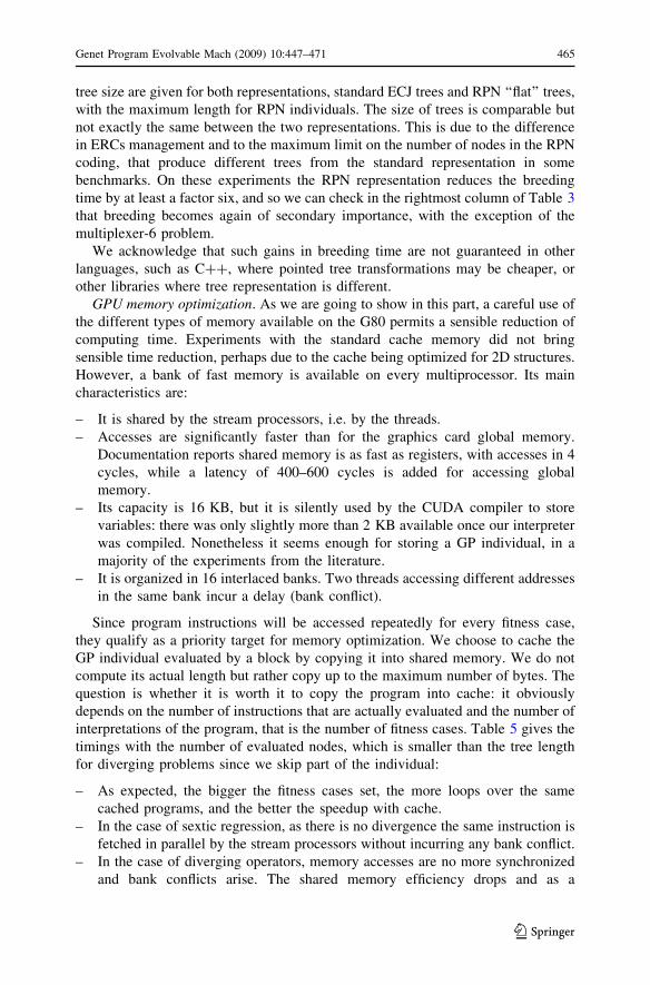
interpretations of the program, that is the number of fitness cases. Table 5 gives the
timings with the number of evaluated nodes, which is smaller than the tree length
for diverging problems since we skip part of the individual:
– As expected, the bigger the fitness cases set, the more loops over the same
cached programs, and the better the speedup with cache.
– In the case of sextic regression, as there is no divergence the same instruction is
fetched in parallel by the stream processors without incurring any bank conflict.
– In the case of diverging operators, memory accesses are no more synchronized
and bank conflicts arise. The shared memory efficiency drops and as a
Genet Program Evolvable Mach (2009) 10:447–471 465
123
consequence a greater number of fitness cases is needed to amortize the filling of
the cache as can be seen on the multiplexers and spiral benchmarks.
– Notice that the speedup also increases with the population size: we attribute this
to memory transfer overheads (included in the evaluation time) that becomes
negligible against the computing time with more individuals.
The fitness cases are also frequently accessed. In all our experiments on GPU the
attributes of the current fitness case being evaluated are copied from global memory
to registers. Alike the deployment of computations on multiprocessors, this memory
management may not be possible with high-level GPU languages.
6.2 Final results
In this sub-section, we report results obtained for full runs with the optimized
BlockGP scheme, i.e. with RPN representation and cached individuals. Following
the practice proposed in [22], we give the speed in terms of the number of GP
operations per second, denoted GPop/s, that measures how many GP nodes have
been computed per second. For example, let us suppose a run duration of 3 s for 5
generations with a population of 2 trees, each of 10 nodes, evaluated on 12 fitness
cases. We also suppose that every node of every evolved tree was effectively
evaluated, i.e. no alternative statement branch have been shortcut and no tree have
been copied from one generation to the next. This hypothetical run would then
exhibit a performance of: ð5� 2� 10� 12Þ=3 ¼ 400 GPop/s.
We focus on the largest population size, 12,500 individuals, which we deem is
the more realistic setting (the trends for smaller populations can be deduced from
the previous section). We also added:
Table 5 Comparison of evaluation times on GPU with and without caching instructions in shared
memory
Population size Sextic regression Multiplexer Spirals
20 64 256 1,024 64 2,048 194
500
Without 0.15 0.18 0.35 1.21 0.45 2.34 0.98
With 0.15 0.16 0.24 0.76 0.86 1.72 1.39
Eval. nodes 47.36 52.97 49.01 59.34 19.77 17.44 60.04
2,500
Without 0.46 0.54 1.43 5.48 2.10 10.74 5.08
With 0.43 0.46 0.91 2.36 3.15 6.12 5.96
Eval. nodes 66.12 63.37 58.05 62.97 21.23 16.91 73.25
12,500
Without 1.76 2.73 8.21 29.58 9.10 45.79 26.44
With 1.46 1.68 3.58 11.32 10.51 27.36 28.94
Eval. nodes 64.48 68.84 68.83 67.22 20.29 14.06 82.95
Timings are given in seconds with the number of evaluated nodes and these are averaged for 30 runs, best
timings are in boldface
466 Genet Program Evolvable Mach (2009) 10:447–471
123
– a version of the sextic benchmark with 100,000 fitness cases;
– the MackeyGlass benchmark as defined in [22]: the objective is to try to predict
a chaotic time series, with the function set fþ;�; �; =g , 128 predefined
constants and 8 inputs as the terminal set. We use a single population with
standard tournament selection of size 2 and no elitism, rather than the grid-based
demes from [22]. This setting generates less fit individuals but this should not
have a significant influence on the running time since their size is in the same
range as in Langdon et al.’s work. Inclusion of this benchmark allows a
comparison with another existing GPU implementation;
– for the MackeyGlass, the size of individuals is limited to 15 nodes, so we have
enough storage for caching several individuals together in fast memory and we
can interpret sequentially several individuals in the same block. This is done
with clusters of 10 individuals and the results are indicated by a star sign—
MackeyGlass*—in the following.
Among these experiments we selected those that could be run on CPU with the
standard ECJ code within reasonable time and memory constraints. The objective of
this comparison is not to establish the superiority of our GPU setting over the
CPU—it was expected since the G80 is announced at 330 Gflops versus 19 Gflops
for our Core-2 6600—but it is intended to provide guidelines about what gains can
or can not be expected from GPUs. Hence we do not present ECJ on CPU with RPN
breeding, the gains brought by RPN breeding being negligible anyway when
evaluation is done on CPU, with the exception of the multiplexer-6. Results are
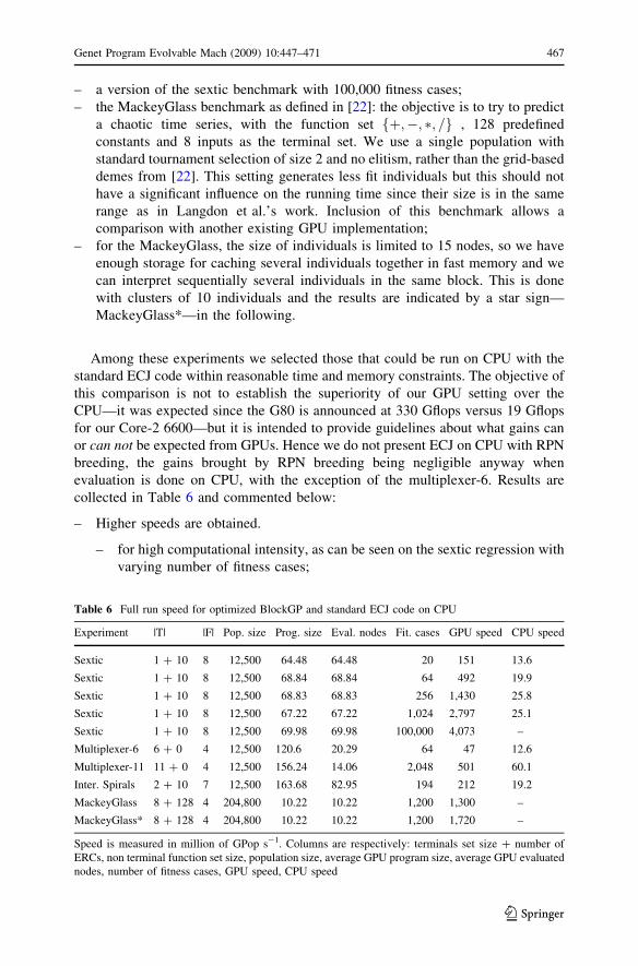
collected in Table 6 and commented below:
– Higher speeds are obtained.
– for high computational intensity, as can be seen on the sextic regression with
varying number of fitness cases;
Table 6 Full run speed for optimized BlockGP and standard ECJ code on CPU
Experiment |T| |F| Pop. size Prog. size Eval. nodes Fit. cases GPU speed CPU speed
Sextic 1 ? 10 8 12,500 64.48 64.48 20 151 13.6
Sextic 1 ? 10 8 12,500 68.84 68.84 64 492 19.9
Sextic 1 ? 10 8 12,500 68.83 68.83 256 1,430 25.8
Sextic 1 ? 10 8 12,500 67.22 67.22 1,024 2,797 25.1
Sextic 1 ? 10 8 12,500 69.98 69.98 100,000 4,073 –
Multiplexer-6 6 ? 0 4 12,500 120.6 20.29 64 47 12.6
Multiplexer-11 11 ? 0 4 12,500 156.24 14.06 2,048 501 60.1
Inter. Spirals 2 ? 10 7 12,500 163.68 82.95 194 212 19.2
MackeyGlass 8 ? 128 4 204,800 10.22 10.22 1,200 1,300 –
MackeyGlass* 8 ? 128 4 204,800 10.22 10.22 1,200 1,720 –
Speed is measured in million of GPop s-1. Columns are respectively: terminals set size ? number of
ERCs, non terminal function set size, population size, average GPU program size, average GPU evaluated
nodes, number of fitness cases, GPU speed, CPU speed
Genet Program Evolvable Mach (2009) 10:447–471 467
123
– when there are no diverging operators: while the GPU implementation is two
orders of magnitude faster than the CPU code on the sextic regression with
1,024 fitness cases, it is only about one order of magnitude on the multiplexer-
11 and the intertwined spirals or on the sextic with 20 fitness cases.
– For the multiplexer-6, the speedup is mainly due to the RPN breeding code (that
runs on CPU), and not to the GPU-ported evaluation.
– The MackeyGlass benchmark does not use diverging operators, but generates
very small programs, so its speed on GPU is smaller than the sextic regression
for a similar number of fitness cases. Nonetheless it is still much faster than the
diverging benchmarks.
– The MackeyGlass* with sequential interpretation of 10 programs per block is
more efficient, and this is due to the smaller number of block creations.
– The difference in speed between the sextic regression with 1,024 and with
100,000 fitness cases indicates the GPU is still far from being saturated with
1,024 fitness cases.
– If we compare these speedups against the ratio of announced gigaflops, we
observe that non diverging problems are particularly well-suited for parallel-
ization and can benefit from the GPU parallel architecture and higher memory
bandwidth, if the computational intensity is high enough. In contrast, the
speedup of diverging problems is below what could have been expected from
raw gigaflops data.
– For both MackeyGlass versions we notice a speedup versus the experiments
reported in [22] where the speed was 895 millions of GPop/s for programs of
size 11. This suggests that our BlockGP algorithm is faster than the automatic
parallelization achieved by the RapidMind toolkit.
7 Conclusions
In this paper, we focus on parallelizing the evaluation phase of Genetic
Programming on the G80 GPU. We propose two population parallel models, based
on an interpreter. We take advantage of the possibilities allowed by CUDA to
reduce the divergence between elementary processors and optimize memory
accesses when interpreting programs. By implementing the GPU evaluation as part
of the well-known Java ECJ library, we intend to offer easy development of GP on
GPU applications, the source code being available at [29].
On our set of benchmarks we observe that:
– The speedup depends on the problem, notably on the presence of diverging
operators and the number of fitness cases.
– For all our benchmarks, dispatching one GP program per multiprocessor yields
speedups even for problems that implement operators with unavoidable
divergence, and it is superior to the scheme that simply associates one program
to each thread.
– The reduced computing time needed by GPU evaluation may promote the
breeding phase as a new bottleneck for common setups.
468 Genet Program Evolvable Mach (2009) 10:447–471
123
– On the G80, fast memory usage can yield improvement up to a factor 3 speedup,
but this is also dependent on the absence of divergence.
The two main critical points that determine the speedup on GPU are the presence
of operators that create divergence and the computational intensity, which is mostly
determined itself by the size of programs and the size of the fitness cases set (see also
[19]). Best results are expected for non diverging function sets, large programs and
large training sets. This implies that the speedup is expected to be rather low if the
fitness is to be computed by a simulator, since it is very likely that a simulator code
will use alternatives or loops. Another difficult case arises when there are both very
few fitness cases and diverging operators, as illustrated by the multiplexer-6. A small
fitness cases set also decreases the advantage of BlockGP over ThreadGP as shown
in Sect. 5. Note that the presence of divergence is of much greater impact than the
delays caused by transferring programs from the host computer to the graphics card.
With other GPUs, the number of elementary processors and the ratio of
elementary processors over multiprocessors will be different in most cases. Of
course the lower the total number of elementary processors is, the lower the
expected performance is. Some other guidelines can be deduced from this work:
– Few elementary processors per multiprocessor means we are closer to a true
MIMD machine and so the advantage of BlockGP over ThreadGP will decrease.
In the meantime, this would be closer to a perfect setting for implementing GP.
– The opposite—many elementary processors per multiprocessor—will generate
more divergence for ThreadGP and will favors BlockGP.
– The preceding item would be true unless the number of fitness cases is so small
that BlockGP cannot fill the stream processors ALUs. In the extreme, there may
be fewer fitness cases than the number of elementary processors or concurrent
threads per multiprocessor; of course this would greatly impair BlockGP.
These remarks lead us to derive other parallel schemes from the two presented
above:
– Two (or more) programs could be executed in parallel on any given block, i.e.
this would implement a crossover between BlockGP and ThreadGP. This way,
program divergence would probably be kept lower than in ThreadGP and
computational intensity would be higher than in BlockGP. This could be an
answer to the last item of the previous paragraph.
– Several programs could also be executed sequentially in each block, as in the
MackeyGlass* benchmark, in order to reduce the number of block creations in
BlockGP and the associated delays. As noted in Sect. 5, one should probably not
decrease below 5 the number of blocks per multiprocessor.
Even if we cannot conclude definitively on how high-level GPU toolkits
parallelize their computations, the MackeyGlass benchmark results suggest that
access to low level architecture is a highly desirable feature. Since the architecture
of the two main GPU makers seems to converge, we could even expect the
development of toolkit facilities common to different families of GPUs, at least for
the distribution of tasks on multiprocessors, and probably also for explicit storage in
Genet Program Evolvable Mach (2009) 10:447–471 469
123
cache or fast memory. This would allow easier portability of high performance code
between GPUs.
SPMD architectures like the G80, built around a set of SIMD cores, exhibit a
lower complexity than true multi-core systems, and are currently very competitive
in terms of price. With new chips performing 64-bits operations, precision issues
should be relieved. With speedups more than a hundred times faster on some
problems, GPUs can offer the opportunity for increasing statistical soundness by
easily sampling hundreds of independent runs. Performance increases could also
open the way to large scale evolution with population sizes in the range of millions
on a standard desktop computer. Thus we think that GPU processing is to be taken
into account by the artificial evolution practitioner.
Some open questions are whether or not it is worth it to port the whole GP
algorithm on GPU, what is the potential of ‘‘crossovers’’ between BlockGP and
ThreadGP as schemed above, and is it possible to speed up diverging operators?
Acknowledgment We thank W. B. Langdon for kindly giving access to his RPN breeding code.
References
1. J.R. Koza, M.A. Keane, M.J. Streeter, W. Mydlowec, J. Yu, G. Lanza, Genetic Programing IV:Routine Human-Competitive Machine Intelligence. (Springer, 2005)
2. C. Gathercole, P. Ross, Dynamic training subset selection for supervised learning in genetic pro-
gramming, in Proceedings of the third Conference on Parallel Problem Solving from Nature, volume866 of Lecture Notes in Computer Science, (Springer, Berlin, 1994), pp. 312–321
3. C. Gathercole, P. Ross, Tackling the boolean even N parity problem with genetic programming and
limited-error fitness, in Proceedings of the Second Annual Conference on Genetic Programming,
(Morgan Kaufmann, Los Altos, 1997), pp. 119–127
4. M. Keijzer, Alternatives in subtree caching for genetic programming, in Genetic Programming 7thEuropean Conference, EuroGP 2004, Proceedings, volume 3003 of LNCS, (Springer, Berlin, 2004),
pp. 328–337
5. C. Fillon, A. Bartoli, A divide and conquer strategy for improving efficiency and probability of
success in genetic programming, in Proceedings of the 9th European Conference on Genetic Pro-gramming, volume 3905 of Lecture Notes in Computer Science, (Springer, Berlin, 2006), pp. 13–23
6. W.B. Langdon, Size fair and homologous tree genetic programming crossovers, in Proceedings ofthe Genetic and Evolutionary Computation Conference, (Morgan-Kaufmann, Los Altos, 1999),
pp. 1092–1097
7. P. Nordin, A compiling genetic programming system that directly manipulates the machine code, in
Advances in Genetic Programming, Chapter 14. (MIT Press, Cambridge, 1994), pp. 311–331.
8. P. Nordin, W. Banzhaf, Evolving turing-complete programs for a register machine with self-modi-
fying code, in Genetic Algorithms: Proceedings of the Sixth International Conference (ICGA95),(Morgan Kaufmann, Los Altos 1995), pp. 318–325
9. P. Tufts, Parallel case evaluation for genetic programming, in 1993 Lectures in Complex Systems,volume VI of Santa Fe Institute Studies in the Science of Complexity, (Addison-Wesley, Reading,
1995), pp. 591–596
10. H. Juille, J.B. Pollack, Massively parallel genetic programming, in Advances in Genetic Program-ming 2, Chapter 17. (MIT Press, Cambridge, 1996), pp. 339–358
11. F. Fernandez, M. Tomassini, L. Vanneschi, An empirical study of multipopulation genetic pro-
gramming. Genet. Programm. Evolvable Mach., 4(1), 21–51, (2003)
12. S.M. Cheang, K.S. Leung, K.H. Lee, Genetic parallel programming: design and implementation.
Evol. Comput., 14(2), 129–156, Summer (2006)
470 Genet Program Evolvable Mach (2009) 10:447–471
123
13. M.L. Wong, T.T. Wong, K.L. Fok, Parallel evolutionary algorithms on graphics processing unit, in
Proceedings of IEEE Congress on Evolutionary Computation 2005 (CEC 2005), vol. 3. (Edinburgh,
UK, 2005), pp. 2286–2293. IEEE
14. Q. Yu, C. Chen, Z. Pan, Parallel genetic algorithms on programmable graphics hardware, in
Advances in Natural Computation, volume 3162 of LNCS, (Springer, Berlin, 2005), pp. 1051–1059
15. Z. Luo, H. Liu, Cellular genetic algorithms and local search for 3-sat problem on graphic hardware,
in IEEE Congress on Evolutionary Computation—CEC 2006., (2006), pp. 988–2992
16. K. Kaul, C.-A. Bohn, A genetic texture packing algorithm on a graphical processing unit, in Pro-ceedings of the 9th International Conference on Computer Graphics and Artificial Intelligence (2006)
17. T.-T. Wong, M.L. Wong, Parallel Evolutionary Computations, Chapter 7. (Springer, Berlin, 2006),
pp. 133–154
18. K.-L. Fok, T.-T. Wong, M.-L. Wong, Evolutionary computing on consumer graphics hardware. IEEEInt. Syst., 22(2), 69–78 (2007)
19. S. Harding, W. Banzhaf, Fast genetic programming on GPUs, in proceedings of the 10th EuropeanConference on Genetic Programming, EuroGP 2007, volume 4445 of Lecture Notes in ComputerScience, (Springer, Berlin, 2007), pp. 90–101
20. S. Harding, W. Banzhaf, Fast genetic programming and artificial developmental systems on GPUs, in
proceedings of the 2007 High Performance Computing and Simulation (HPCS’07) Conference.
(IEEE Computer Society, 2007), p. 2
21. D.M. Chitty, A data parallel approach to genetic programming using programmable graphics hard-
ware, in Proceedings of the 2007 Genetic and Evolutionary Computing Conference (GECCO’07),(ACM Press, London, UK, 2007), pp. 1566–1573
22. W.B. Langdon, W. Banzhaf, A SIMD interpreter for genetic programming on GPU graphics cards, in
Proceedings of the 11th European Conference on Genetic Programming, EuroGP 2008, volume 4971of Lecture Notes in Computer Science ed by M. O’Neill, L. Vanneschi, S. Gustafson, A.I.E. Alcazar,
I. De Falco, A. Della Cioppa, E. Tarantino, (Springer, Naples, 2008) pp. 73–85
23. D. Robilliard, V. Marion-Poty, C. Fonlupt, Population parallel GP on the G80 GPU, in Proceedingsof the 11th European Conference on Genetic Programming, EuroGP 2008, volume 4971 of LectureNotes in Computer Science ed by M. O’Neill, L. Vanneschi, S. Gustafson, A.I.E. Alcazar, I. De
Falco, A. Della Cioppa, E. Tarantino, (Springer, Naples, 2008), pp. 98–109
24. W.B. Langdon, A.P. Harrison, GP on SPMD parallel graphics hardware for mega bioinformatics data
mining, Soft Computing, (2008). Special Issue. On line first
25. S. Harding, Evolution of image filters on graphics processor units using cartesian genetic pro-
gramming, in 2008 IEEE World Congress on Computational Intelligence ed by J. Wang, (IEEE
Computational Intelligence Society, IEEE Press, Hong Kong, 2008)
26. D.T. Anderson, R.H. Luke, J.M. Keller, Speedup of fuzzy clustering through stream processing on
graphics processing units, in 2008 IEEE World Congress on Computational Intelligence ed by
J. Wang, (IEEE Press, Hong Kong, 2008), pp. 1101–1106
27. S. Luke, L. Panait, G. Balan, S. Paus, Z. Skolicki, E. Popovici, K. Sullivan, J. Harrison, J. Bassett,
R. Hubley, A. Chircop, ECJ 18—a Java-based evolutionary computation research system. Available
at http://www.cs.gmu.edu/eclab/projects/ecj, (2008)
28. P. Sanders, Emulating MIMD behavior on SIMD machines, in Proceedings of International Con-ference on Massively Parallel Processing Applications and Development, (Elsevier, Delft, 1994).
29. D. Robilliard, V. Marion-Poty, C. Fonlupt, GPURegression: Population parallel GP on G80 GPUs—
ECJ compatible code. Available at http://www.lil.univ-littoral.fr/*robillia/GPUregression.html,
(2008)
30. A.V. Aho, R. Sethi, J.D. Ullman, Compilers—Principles, Techniques and Tools. (Addison-Wesley,
Reading, 1986)
31. J.R. Koza, Genetic Programming II: Automatic Discovery of Reusable Programs. (The MIT Press,
1994)
32. J.R. Koza, Genetic Programming: On the Programming of Computers by Means of Natural Selection.
(The MIT Press, 1992)
33. K.J. Lang, M.J. Witbrock, Learning to tell two spirals apart, in Proceedings of the 1988 ConnectionistSummer Schools, ed by Morgan-Kaufmann (1988)
34. W.B. Langdon, Evolving programs on graphics cards—C?? code. Available at http://www.cs.ucl.
ac.uk/external/W.Langdon/ftp/gp-code/gpu_gp_1.tar.gz, (2008)
35. M. Brameier, W. Banzhaf, Linear Genetic Programming. Number XVI in Genetic and EvolutionaryComputation. (Springer, 2007)
Genet Program Evolvable Mach (2009) 10:447–471 471
123


