Economic Impacts of Integrated Pest Management in Developing Countries: Evidence from the IPM CRSP
Tatjana Hristovska
Thesis submitted to the faculty of the Virginia Polytechnic Institute and State University
in partial fulfillment of the requirements for the degree of
Master of Science In
Agricultural and Applied Economics
George W. Norton, Chair Daniel B. Taylor
Jeffrey R. Alwang
April 13, 2009 Blacksburg, VA
Keywords: IPM CRSP, Economic surplus, impact assesment, Albania, Ecuador, Uganda, adoption analysis, Bangladesh

Economic Impacts of Integrated Pest Management in Developing Countries:
Evidence from the IPM CRSP
Tatjana Hristovska
(Abstract)
Farmers around the world rely on IPM practices in order to increase their yields and
reduce their losses due to pests. Assessing the impacts of previous IPM CRSP studies is
crucial for successful continuance of the program and to provide meaningful
recommendations to farmers. This thesis summarizes previous IPM CRSP impact studies,
and provides additional impact assessments of IPM practices developed on the program.
Scientist-questionnaires were sent to scientists in each IPM CRSP site around the world.
Using the data from the questionnaire responses in combination with additional
secondary information on elasticities, prices and quantities, economic surplus analyses
were conducted. The tomato IPM program in Albania, the plantain IPM program in
Ecuador, and the tomato IPM program in Uganda resulted in net present values of
approximately $8 million, $7 million and $1 million, respectively. Sensitivity analyses
for each case were also conducted, and net benefits ranged from $5 to 23 million in
Albania, from $4 to 7 million in Ecuador, and from $0.03 to 3 million in Uganda.
Additionally, an ordered probit analysis was conducted to determine the factors affecting
adoption of IPM technologies in Bangladesh. The level of education, being a female, IPM
training and awareness of pesticide alternatives were found to have positive and
statistically significant impact on the adoption of IPM technologies in Bangladesh.

iii
Table of Contents Chapter I. Introduction.........................................................................................................1
I.I. Integrated Pest Management ..................................................................................1 I.II. Problem Statement ................................................................................................3 I.III. Objectives ............................................................................................................4 I.IV. Hypotheses ..........................................................................................................5
I.V. Organization of Thesis..........................................................................................5 Chapter II. Literature Review ..............................................................................................6 II. I. Descriptive summary of impacts of IPM in specific regions...................................6 II.II. Additional IPM CRSP Impact Studies ..................................................................11 II.II.A. Africa .................................................................................................................11 II.II.B. Asia ....................................................................................................................15 II.II.C. Eastern Europe ...................................................................................................22 II.II.D. Latin America ....................................................................................................23 Chapter III. Methods..........................................................................................................26 III.I. Benefit-Cost Analysis.............................................................................................33 III.II. Budgeting ..............................................................................................................36 Chapter IV. Results of the Additional Analysis of IPM CRSP Impacts............................37 IV.I. Tomato IPM Program in Albania..........................................................................38 IV.II. Plantain IPM Program in Ecuador .......................................................................41 IV.III. Tomato IPM program in Uganda........................................................................44 Chapter V. Factors Determining Adoption of IPM Technologies in Bangladesh .............49 V.I. Basic Background Information...............................................................................49 V.II.Technology adoption discussion and literature review of IPM adoption...............50 V.III. The econometric model: an ordered probit ..........................................................54 V.IV. Determinants affecting adoption..........................................................................58 V.V. Results and Conclusions .......................................................................................65 Chapter VI. Conclusions and Limitations..........................................................................69 VI.I. Implications for further research ...........................................................................71 References..........................................................................................................................73 Appendices.........................................................................................................................77
iv
List of Tables Table 1: Summary Table of benefits from the IPM CRSP impact studies….................. 25
Table 2: Summary of the results from the economics surplus analysis and sensitivity analysis for tomato IPM in Albania.....................................................................................41
Table 3: Summary of the results from the economics surplus and the sensitivity analysis of the Plantain IPM Program in Ecuador.............................................................................44
Table 4: Summary of the original and two sensitivity analysis for the Tomato IPM Program in Uganda…………………………………………………………………............46
Table 5: Summary of the case 1 and case 2 economic surplus analyses conducted in the case of the Tomato IPM Program in Uganda…................................................................48
Table 6: Statistical summary of variables............................................................................65
Table 7: Summary of the models’ results............................................................................66
List of Figures Figure 1: Consumer and Producer Surplus....................................................................... 27 Figure 2: Research benefits, size, and distribution due to trade (large country exporter innovates, no technology spillover).................................................................................. 29
Figure 3: Research benefits size and distribution due to trade (large country exporter innovates, with technology spillover)...............................................................................32
List of Appendices Appendix A: A sample scientist-questionnaire................................................................ 77 Appendix B: The variables used in the economic surplus analysis...................................79 Appendix C: The economic surplus analysis Excel table for Tomatoes – Albania...........82 Appendix D: Sensitivity analysis Excel table for Tomatoes – Albania.............................82 Appendix E: Economic Surplus analysis Excel table for Plantain – Ecuador...................83 Appendix F: Sensitivity Analysis Excel table for Plantain, Ecuador................................83 Appendix G: Economic Surplus Analysis Excel table for Tomatoes, Uganda.................83 Appendix H: Sensitivity Analysis Excel table for Tomatoes, Uganda..............................84

v
Acknowledgements
First, I would like to thank my advisor Dr. George Norton. Dr. Norton, thank you for
giving me the opportunity to work on this project, I have learned a lot from it. Thank you
for your patience, for your comments and suggestions. Thank you for being available and
welcoming every time when I had questions.
I also would like to thank Dr. Dan Taylor and Dr. Jeffery Alwang for their helpful
insights and corrections of my work.
Also, a special thank you goes to the Agriculture Office within the Bureau for Economic
Growth, Agriculture, and Trade (EGAT) of the U.S. Agency for International
Development, under the terms of the Integrated Pest Management Collaborative Research
Support Program (IPM CRSP) (Award No. EPP-A-00-04-00016-00). Thank you for the
support and making this thesis possible.
I would like extend my gratitude to the research scientists from the IPM CRSP sites in
Albania, Ecuador and Uganda for participating in the individual scientist-questionnaires.
Thank you: J. Tedeschini, V. Jovani, B. Alushi, Carmen Suarez-Capello, Dr. Namirembe-
Ssonko, Dr. Michael Otim, Dr. Sophie Musana, Mr. Zach Muwanga, Mr. Basil Mugonola
and Dr. Jackie Bonabana. Your responses have given me valuable information and are
the base of my analysis, thank you.

vi
I’m indebted to Atanu Rakshit for letting me use the data from his Bangladesh survey and
also for helping me with my questions about the survey.
My special thanks go to my friends from the AAEC department (Anna, Amanda, Todd,
Adam, Zack, Pricilla, and Ranju) and my friends from Macedonia (Biljana and Irena) –
for their support and all the wonderful moments together.
My highest gratitude goes to Vuko. Thank you for being my soul-mate and best friend,
thank you for your support, advice, for all the laughs, hugs. Thank you for loving me and
being with me.
My deepest gratitude goes to my family. Mama, Tato and Stefan, thank you for your
unconditional love and support. Thank you for always being there for me in any way
possible. Even though we are miles apart you are always in my heart and my thoughts.

vii
Dedicated to Mom, Dad and Stefan
~Thank you for being the best family ever~
And to Vuko
~Thank you for being by my side~
Посветено на Мама, Тато, и Стефан
~затоа што сте најдобрата Фамилија~
1
Chapter I. Introduction
Agriculture is an important part of every economy, especially in developing countries
where most of the people depend on agriculture as their primary source of income.
According to the United States Agency for International Development (USAID 2007),
more than a billion people live on less than a dollar per day; approximately 70 percent of
which live in rural areas and spend all or part of their time farming or raising livestock.
Although agriculture is very important part of each country, it is not as reliable as it needs
to be in less developed countries to be a dependable source of income. A lot of the
farmers in developing countries often do not produce enough to feed their own families.
USAID has stated that increasing the productivity of the agricultural sector is a crucial
goal (USAID 2007). Some factors that affect agricultural productivity and the variability
of production from year to year are weather, insects and diseases.
I.I. Integrated Pest Management
Numerous programs around the world work toward increasing agricultural productivity
and improving the lives of farmers, one of which is Integrated Pest Management (IPM).
IPM is a systems approach that works toward reducing the negative productivity effects
caused by pests, but without harming the environment in that process (IPM CRSP,
2008a).
The Environmental Protection Agency (EPA) has defined IPM as an effective and
environmentally sensitive approach to manage pests that relies on a combination of
common-sense practices (EPA, 2007). Using current information about pests and the

2
environment, IPM combines available pest control methods to manage pest damage by
the most economical means, and with the least possible harm to people, property, and the
environment. According to the EPA (2007), IPM practices can be implemented in
agricultural and non-agricultural settings (like the home, garden, and workplace).
According to Norton and Mullen (1994), IPM is an approach which uses increased
information to make pest control decisions, and also uses multiple tactics to manage pest
populations in a way that is both economically efficient and ecologically sound.
IPM practices natural, environmentally friendly approaches that increase agricultural
productivity. Examples of IPM practices are adoption of pest-resistant varieties of crops;
biological and physical control methods; environmental modification; biopesticides; and
when absolutely necessary, non-residual, environmentally-friendly and low mammalian-
toxic chemical pesticides (IPM CRSP 2008a).
The Integrated Pest Management, Collaborative Research Support Program (IPM CRSP),
started in September 1993 and is funded by USAID. The objective of the IPM CRSP is to
develop and implement IPM practices that can help increase the standard of living as well
as improve the environment in various countries around the world. The objectives are
achieved through research, education for behavioral changes, policy and institutional
reforms and the development of sustainable, resource-based local enterprises (IPM CRSP
2008b). Over the years, the IPM CRSP has helped numerous countries in Eastern Europe,
Africa, Latin America, Asia and the Caribbean. There have been several regional projects
specifically tailored to a particular problem in a particular country, but there are also
global programs.

3
I.II. Problem Statement
There is a need for a standardized assessment of impacts across all projects on the IPM
CRSP. According to Norton et al. (2005, pp.241) “impact assessment is crucial for
making meaningful recommendations to farmers, for demonstrating the value of IPM
programs, and for assessing who will adopt so that programs can be tailored to audiences
to obtain consistency with program goals.” There has been an uneven distribution of IPM
CRSP impact assessment studies and projects, therefore it is necessary to provide more
up to date impact assessments for the countries that have not been studied extensively, for
example Uganda, Albania and Ecuador.
Some of the effects resulting from implementing IPM practices can be: reduced pesticide
use, reduced crop losses, reduced loss of biodiversity, reduced damage to natural
ecosystems, increased farmer income, improving research and education capabilities, and
increased involvement of women in decision-making. Each of these effects has a specific
type of economic impact, a summary report for all the economic impacts has not been
prepared. A summary report is needed to inform stakeholders of the overall joint progress
of the IPM CRSP over the years. This type of report will help participants, project
planners, and funding agencies in their future decisions. It can serve as a general data
base for information on each project, while more detailed information for each project
will still be available.
Dissemination of IPM technologies is an important part of the IPM CRSP efforts. Despite
the positive effects from IPM technologies, and the efforts of numerous scientists,
4
students, non-government officials, volunteers etc., farmers are not always aware or fully
informed about the existence of and all the effects resulting from the adoption of IPM
technologies. There are different factors that affect adoption, and analyzing those factors
provides useful information that can help improve the adoption of IPM technologies. Due
to the newly available up-to-date data and the changing conditions in each country,
conducting adoption analyses is necessary. Analyzing the factors affecting adoption of
IPM technologies is especially important in the case of less developed countries (LDCs)
because as Feder, Just, and Zilberman (1985) point out, the majority of the population
depends on agriculture and the adoption of new technologies has proven to increase
agricultural production and income. One of the poorest nations in the world, Bangladesh,
is one of the primary sites on the IPM CRSP. Analyzing the factors that affect adoption
of IPM technologies is an important step toward designing strategies for scaling up the
spread of IPM technologies to Bangladeshi farmers.
I.III. Objectives
The two primary objectives of this study are to measure and summarize the impacts of
the IPM CRSP from its beginning to the present, and also to analyze the factors affecting
the adoption of IPM technologies in the case of Bangladesh. This study will include a
large number of IPM CRSP projects and will provide a consistent analysis of the projects.
It will:
I. Review and summarize results from previous impact studies on the IPM
CRSP
5
II. Assess the impact of specific IPM CRSP programs in Albania, Uganda and
Ecuador
III. Identify factors that affect adoption of IPM technologies in Bangladesh.
I.IV. Hypotheses
1. IPM practices result in a positive Net Present Value (NPV) of benefits in
every country where the IPM CRSP is working.
2. The adoption of IPM increases as the level of education increases, if the
farmer is female, as the number of working family members increases, as the
percentage of farm income from total annual income increases, if the farmer
had an IPM training, and if farmer is aware of pesticide alternatives.
The adoption of IPM practices decreases as the farmers’ age increases, as the
farm size increases, and as the distance (km) to the nearest extension agent
increases.
I.V. Organization of Thesis
Chapter II is a literature review of IPM CRSP impact studies by region (Africa, Asia,
Eastern Europe). Chapter III discusses the methods used in the impact studies. Chapter
IV includes additional impact analysis (for tomatoes in Albania and Uganda, and
plantains in Ecuador). Chapter V is devoted to analyzing the factors affecting the
adoption of IPM technologies in Bangladesh. Chapter VI provides a summary,
conclusions and limitations.
6
Chapter II. Literature Review
The IPM CRSP has published numerous work plans, trip reports, annual reports, articles,
books and other documents. This chapter briefly describes the results from previous IPM
CRSP impact studies beginning with those summarized in the book “Globalizing
Integrated Pest Management: A participatory research process” published in 2005.
Section II.I presents the basis for better understanding section II.II, which provides
specific information about IPM CRSP impacts by country. Since the publication of the
book in 2005, the number of countries where the IPM CRSP has presence has increased.
Some of the new participant countries are: Indonesia, Moldova, Ukraine, Uzbekistan,
Tanzania and Kenya. Currently the IPM CRSP is in 32 countries (IPM CRSP 2008).
II.I. Descriptive summary of impacts of IPM in specific regions
Asia (Miller et al. 2005)
The Philippines and Bangladesh face numerous pest problems and have large populations
to feed. Vegetable IPM programs that include participatory appraisals (PA), stakeholder
meetings, monitoring, prioritizing of pest problems etc., have been undertaken in both
countries. The IPM CRSP has provided assistance in diagnosing insect, disease, and
weed problems that farmers are having difficulty managing. The IPM CRSP has worked
on developing environmentally safe and economically sound approaches for managing
pests in eggplant (brinjal), tomato, okra, cucurbits, and cabbage in Bangladesh, and in the
Philippines in rice and other vegetable-vegetable cropping systems focused on onion and
eggplant. IPM CRSP research has addressed some of the most economically harmful
insects and diseases. Appropriate technologies and approaches have been developed
7
which provided the farmers with “tools” to reduce their pest losses. Successful IPM
programs require interdisciplinary collaboration among scientists, economists, and local
farmers. Successful technologies that are being adopted include using disease and insect
resistant varieties, grafting for tomato and eggplant for bacterial wilt resistance,
pheromones and/or bait traps in cucurbits and onion production. Also, various weed-
management practices are being adopted such a hand weeding in combination with
reduced pesticide use, stable seedbed technique (a soil conservation tactic that reduces
erosion) etc. IPM CRSP research on the most important pest in eggplant, Leucinodes
orbonalis or eggplant fruit and shoot borer (EFSB), showed that simply by removing the
damaged fruits and shoots during harvest rather than throughout the season, labor costs
could be reduced and there could be a net incremental benefit of $2,500/ha for weekly
removal and $1,000/ha for biweekly removal. Adoption of a reduced insecticide
application practice can reduce insecticide applications from 30-50 to six in a cropping
season. The IPM CRSP also found that using larval and pupal parasitoid Trathala
flavoorbitalis, can reduce EFSB infestation of the 1st instar larvae by 91%. Bacterial wilt
(BW) is caused by Ralstonia solanacearum and causes tremendous losses in eggplant
production. The yield losses for farmers in Bangladesh are often in excess of 50%, while
in Central Luzon, Philippines yield losses can be from 30 to 80%. The use of bacterial
wilt-resistant Solanum melongena line showed increased resistance to BW of 20 to 30%
(Miller et al. 2005). These were just a few examples of the many results obtained
showing the role of IPM in improving the livelihood of farmers and people in the
Philippines and Bangladesh.

8
Africa (Erbaugh et al. 2005)
IPM programs in Africa require a different approach than in Asia. Developing IPM
programs that help small-farmers has been challenging. Studies have found that intensive
exposure to IPM practices through farmer-field schools increases the chances of
adoption. Participatory IPM has had some difficulties with respect to cost, and
communication issues between the scientists and farmers in distant areas. The
development of new technologies has been proposed to be completed in two stages due to
the necessity to expand the number of farmers reached. The first stage is to develop the
new technology and the second stage involves adapting the technologies to specific sites
and providing the technologies to farmers. In Mali in 1999, an innovative approach was
started to control Striga parasitism using herbicide application on sorghum seed, which
resulted in reduced number and dry weight of Striga plants attacking sorghum by over 50
percent. In Uganda and Kenya, cowpea emerged as an important export crop and the crop
that is most likely to be sprayed with chemical pesticides. The IPM CRSP developed
packages that effectively reduced insect pests on cowpea and increased the grain yield by
over 90 percent.
Latin America (Alwang et al 2005) and the Caribbean (Lawrence et al 2005)
The use of IPM practices in Latin America showed significant reduction of insects and
diseases which can have positive effects on the socio-economic status of the people in the
countries in question (Alwang et al 2005). Implementation of such IPM practices and
institutionalizing the pest-management programs can ensure more sustainable export
markets. Farmer-field schools have proven to effectively increase the adoption of IPM
9
technologies and are being redesigned to reach larger numbers of farmers. In Guatemala
the IPM CRSP worked on reducing pesticide residues and improving snowpea quality.
One IPM tactic included pest scouting for insects, which resulted in a 61 percent
reduction in pesticide use and a 6 percent increase in average total yield. Another
effective IPM package was developed for tomato. IPM production costs for tomato were
$700/ha lower, profits were $1,700/ha greater, and pesticide use decreased from more
than 23 sprays to 13 sprays (Weller et al., 2002). In the case of potato production in
Carchi, Ecuador it was found that the net benefits from an IPM package (involving: late-
blight resistant variety (INIAP-FRIPAP99), traps and limited leaf spraying for Andean
weevil, monitoring and limited spraying for the tuber moth, and other low-input controls)
resulted in $643 per ha net benefits compared to local practices. Another impact study of
late blight resistance in the North Region in Ecuador found that the net present value of
research was $34 million (Alwang et al 2005).
Although Jamaica was the primary IPM CRSP site in the Caribbean, there has been an
IPM impact on the broader region as well (Lawrence et al 2005). Workshops, on-farm
demonstrations and variety trails, all have had positive impacts on reducing the farmers’
losses and in educating farmers. A prototype web-based pest monitoring system was also
set up as a part of the IPM CRSP program. This type of monitoring system can be used
for pest surveillance in the future in other IPM CRSP sites. IPM also influenced trade in
the Caribbean, by introducing improved varieties and reducing their losses. The three
main case studies presented by Lawrence et al (2005) were sweet potato, hot pepper and
callaloo. In the sweet potato case study, the factors being assessed included: weevil
10
populations, usage of cultural practices, trap maintenance, and resultant crop losses. A
significant yield loss difference due to weevil was found between the IPM users and
cultural practices users, averaging 4% and 13%, respectively. In the case of pheromone
traps (for male weevils) there was a significant difference in the number of pests caught
on 0.1 ha of sweet potato resulting in mean weevil catch of 22 and 779, for IPM users and
cultural practices users, respectively. In the case of hot peppers in Jamaica it was found
that weekly application of JMS Stylet-Oil® using a backpack mist blower delayed the
field spread of Tobacco etch virus (TEV) for seven days and reduced TEV incidence by
24% compared to unsprayed plots (McDonald, 2004). It was also found that using Stylet-
Oil® together with reflective mulch delayed the TEV incidence in pepper plots for more
than two months, even with inoculum pressures of 33-67% infection from surrounding
plants (Lawrence et al 2005).
Eastern Europe (Pfeifer et al 2005)
The IPM CRSP project has also functioned in Albania (Pfeifer et al 2005). A project was
conducted to measure IPM impacts on the olive fruit fly. Economic cost-benefit analysis
of olives under IPM practices was conducted. Although different methods were used
(harvest timing, pruning and timing of copper sprays, vegetation management and
pheromone based management of the olive fly), all IPM methods were feasible and
showed net profits compared to no-spray and a hypothetical full spray program. A harvest
timing/olive fruit fly study produced the highest net gains of $21.1 million, the
pheromone based olive fruit fly management was second, with gains of $11 million, the
weed management practice was on the third place with gains of $4.3 million, and the

11
pruning/copper sprays resulted in gains of $2.5million. Sixty three percent of these gains
were attributed to yield gains and the rest from quality gains.
II.II. Additional IPM CRSP Impact Studies
This section reviews additional economic impact assessments of the IPM CRSP. Antle
and Capalbo (1995), define the economic impact assessment of integrated programs as
“an application of the economic tool of benefit cost analysis, combined with appropriate
data and models from production economics, environmental science, and health science.”
The studies reviewed in this section range from the beginning of the IPM CRSP in 1993
until today. Each study is reviewed individually. There are four sub-categories in this
section, the sub-categories refer to the different geographical regions. Depending to the
country in which the studies were conducted, each study is placed in one of the three sub-
categories. Studies that contain a mix of counties were divided and each part of the study
was placed in the appropriate sub-region.
II.II.A. Africa
Moyo et al. (2007) conducted partly ex-post and partly ex-ante analysis in Uganda that
focused on poverty reduction as a result of research to develop a peanut-disease resistant
seed. An economic surplus analysis was combined with analysis of household level data,
in order to estimate the poverty reduction. The following three steps were undertaken
during the economic surplus analysis:
a. The unit cost reduction associated with adopting the new seed technology was
calculated

12
b. Information for the expected rate of adoption was gathered based of other new
technologies being adopted in the past and the fact that 15 percent of the farmers have
already adopted the improved seed in the first two years since its release.
c. The poverty change resulting from technology adoption was estimated by computing
the household level value of welfare (income and consumption per capita) and
comparing the income to the poverty line, determining potential adopting households
and the welfare change by level of adoption and adding up the change in the number
of poor households/people due to adoption.
The poverty reduction data were collected through the Uganda National Household
Survey, conducted with the help of the International Food Policy Research Institute
(IFPRI) and the Uganda Bureau of Statistics. The data set consisted of 2,949 peanut
producing households. The effects of adoption of the new technology were spread over a
fifteen year period starting in May 2001. Changes in poverty were calculated using
measures of the Foster-Greer-Thorbecke (FGT) type. The FGT indices are commonly
used because they are additively decomposable with population share weights, which
allows evaluation of impacts of agricultural and other policies on subgroups such as
peanut producers. The results indicated a modest 5-6 percent increase in income in an
open economy and 2.3 to 2.5 percent in a closed economy case. The beneficiaries of this
study are the people from Uganda. Both consumers and producers gain from the
implementation of the technology. Producers have higher yields and income and
consumers have lower prices. Since poor people spend most of their income on food, they
benefit a lot from the technology. Getting poor people closer to the poverty line is a step
forward compared to the current situation they live in. Finally, in an open economy
13
model with 100 percent adoption, the poverty severity index decreases by 2 percent,
which represents a 10.5 percent decline in poverty severity. These numbers are lower for
a closed economy model. The net present value (aggregate net returns to the research) for
an open economy is estimated to be $43.0 and $35.6 million at 3% and 5% discount rates,
respectively. The beneficiaries are the producing households, while the costs are borne by
the research sponsors. In a closed economy, the net benefits are estimated to be $41.1 and
$34.0 million at 3% and 5% discount rates, respectively. The beneficiaries in this case are
both producing and consuming households. Sensitivity analysis was also conducted. At
the 25 percent adoption rate, the NPV increased both in the case of an open economy
model to $62.0 and $51.3 million at 3 and 5 percent discount rates, respectively and for a
closed economy to $58.3 and $48.2. (Moyo,et al. 2007).
Nouhoheflin et al.(2009) conducted a research study on tomatoes in Mali. According to
the author tomatoes are one of the most important crops in Mali and are grown
throughout all the seasons. Despite of the wide usability and trade in West Africa,
tomatoes are susceptible to pest and diseases which cause losses of about 30-50%, while
tomato viruses such Bemissia tabaci, vectored by the whitefly can cause losses of up to
90-100%. Nouhoheflin et al. (2009) summarized the baseline survey results and assessed
the economic impacts of the efforts to reduce the tomato virus problem. The baseline
survey provides socio-demographic data and information about the tomato production
and pest problems in Mali. In order to address the tomato virus problems in Mali, IPM
technologies and biotechnology (GMO) were developed. The economic surplus approach
was used to assess the impacts of those technologies on consumers and producers. Few

14
different scenarios were examined. Under the first scenario when both IPM strategies and
GMO technologies are used in a closed economy, the total economic surplus was
estimated to be approximately $1.35 million, out of which approximately $0.9 million
was consumer surplus and $0.45 million were gains to producers. The NPV of the
benefits from adopting IPM technologies and GMO strategies over 15 years was
estimated to be about $11.64 million, while the IRR was estimated to be 102%. The
second scenario considered only the adoption of IPM strategies in a closed economy. The
total economic surplus in this case was about $1.16 million, out of which about $0.77
million were gains to consumers and $0.38 were gains to producers. The NPV of the
benefits from adoption of IPM strategies over 15 years was approximately $10.3 million
and the IRR was 134%. The third closed economy scenario only considered adoption of
GMO’s, which generated a total economic surplus of approximately $0.2 million, out of
which about $0.13 million were gains to consumers and about $0.07 were gains to
producers. The NPV of the benefits induced by GMO technologies over 15 years was
estimated to be approximately $1.5 million, while the IRR was estimated to 50%.
The three cases were also estimated in an open economy, which changes the results.
Under the first scenario (IPM practices + GMO technologies), the total economic surplus
was $1.44 million, while under the second scenario (only IPM practices) the total
economic surplus is $1.23 million, and under the third scenario (only GMO’s) the total
annual economic surplus is $0.21 million. The NPV of benefits from technology adoption
are: $12.4, $10.9 and $1.6 million, respectively (Nouhoheflin et al. 2009).

15
Debass (2000) assessed the economic impacts of IPM CRSP activities in Bangladesh and
Uganda using geographical information system (GIS) applications and economic surplus
analysis. Bangladesh and Uganda depend on agriculture, and numerous pests, insects,
diseases etc., affect the yields and increase the costs to farmers. Using pesticides has
drawbacks because farmers tend to overuse them which harms the environment and
people’s health. The results from Debass’s analysis were divided in two sections, the
results from Uganda are presented in this section and the results from Bangladesh are
presented in the following section regarding countries in Asia. In Uganda the IPM CRSP
is mainly focused on beans, maize, sorghum, and groundnuts. The main goals are increasing
yields, lowering costs, and improving the life of farmers and the overall population. In order
to measure the effects of the IPM CRSP in Uganda, partial budget and economic surplus
models were used. GIS was used to measure the transferability of IPM technology across
regions. The results from this study were divided by region in each country. In Uganda,
under the baseline scenario the overall net present value for beans using the seed dressing
practice (chemicals mixed with seed grain to prevent incest and rodent infestation and
infection by fungi) was approximately $202 million and the internal rate of return was
250%. Under the baseline scenario, the overall net present value for maize (in Uganda)
using the Longe-1 variety was $36 million and the internal rate of return was 250%. This
study found that IPM practices implemented through the IPM CRSP are more viable and
profitable than the conventional practices used by the local farmers (Debass 2000).
II.II.B. Asia
Debass (2000) also assessed the economic impacts of IPM CRSP activities in Bangladesh
where the IPM CRSP research is focused on eggplant (birnjal), cabbage, cauliflower, and

16
gourds. The goal of the IPM CRSP program in Bangladesh is increasing yields, lowering
costs, and improving the life of farmers and the overall population. In order to measure the
effects of the IPM CRSP in Bangladesh partial budget and economic surplus models were
used. GIS was used to measure the transferability of IPM technology across regions. The
results from this study were divided by region in each country. Under the baseline
scenario, the overall net present value for eggplant using the neem leaf powder practice in
Bangladesh was approximately $29 million and the internal rate of return was 684%.
Under the baseline scenario, the over all net present value for cabbage using the hand
weeding practice in Bangladesh was approximately $26 million and the internal rate of
return was 696%. The net present value and the internal rate of return change with the
adoption rates. (Debass 2000)
Mamaril and Norton (2006) conducted economic surplus analysis for transgenic pest
resistant rice in the Philippines and Vietnam. Rice is a staple food in Asia, and poor
people obtain more than half of their calories from rice. The Bt rice contains soil
bacterium Bacillus thuringiensis (Bt), that has been especially developed for stemborer
control. The Philippines is a net importer of rice and most of the imports come from
Vietnam. A partial equilibrium rice model was constructed for the Philippines, Vietnam
and the rest of the world (ROW). The Philippines has the strongest bio-technology
research program in Southeast Asia and also has a bio-safety program in place, while
Vietnam is best positioned to take advantage of Bt rice sometime after the Philippines.
The total projected economic gains (in 2000 prices) from adopting Bt rice under the
baseline scenario in 2005 in the Philippines and in 2008 in Vietnam were $619 million
(range from $306-717 million), $270 million (range from $136-276 million) in the

17
Philippines, $329 million (range from $159-415 million) in Vietnam, and $20 million
(range from $10-26 million) at the ROW. The results differ if both countries
simultaneously adopt the Bt rice, with Vietnam benefits increasing significantly to $415
million. Several different scenarios have been developed and each scenario offers
different results although the results lie within the ranges mentioned above (Mamaril and
Norton 2006).
Mishra (2003) assessed the impacts of Bt Eggplant in Bangladesh, the Philippines and
India. Eggplant is one of the most important vegetables in Bangladesh, the Philippines
and India, but it is highly susceptible to diseases. An economic surplus model for a closed
economy was simulated. Under the baseline adoption scenario, it was estimated that yield
would increase by 15 percent, and the input costs after the adoption of the BT eggplant
would decrease by 30 percent. Under the conservative set of assumptions, the minimum
benefits would be a 15 percent increase in yield and a 15 percent decrease in input costs,
and India would gain about $279 million (net present value), Bangladesh would gain $25
million (net present value), and the Philippines would gain $19 million (net present
value). Under the simulation with a base level of 15 percent increase in yield and 30
percent decrease in input costs, India would gain $411 million (net present value),
Bangladesh would gain $37 million (net present value), and the Philippines would gain
$28 million (net present value). The maximum benefits, 45 percent increase in yield and
45 percent decrease in input costs, would result in gains of $773 (net present value)
million in India, $69 (net present value) million in Bangladesh, and $53 (net present
value) million in the Philippines. In all cases, producers would gain 43 percent of the
18
surplus and consumers gain would 57 percent. The baseline scenario simulation assumes
a maximum adoption rate of 35 percent. If the adoption rate changes, it consequently
changes the benefits to the countries in question. The benefits to each country are also
affected by the demand and supply elasticities (Mishra 2003).
Cuyno (1999) conducted an economic evaluation of the health and environmental
benefits of an IPM program (IPM CRSP) in the Philippines. Agricultural pests cause
significant damage to farm yields and incomes, but the pesticides do not solve the
problem. First of all, they increase the costs to the farmers and harm the environment and
the health of the farmers and the people around the farm area. Measuring the benefits
from the IPM CRSP program is crucial because it affects both the people and the
environment, and helping people and the environment is one of the basic objectives of the
IPM CRSP. The methods used to measure the benefits are contingent valuation (CV) and
benefit cost analysis (B-C). The analysis is complex, at first the impacts are categorized
as: impacts on human health, impact on beneficial insects, impact on aquatic species,
impact on farm animals, and impact on birds. Then, environmental impact assessment of
pesticide use is conducted, the IPM CRSP technology adoption levels are
predicted/estimated, and the IPM CRSP impacts on pesticide reduction are estimated.
Then, society’s willingness to pay is estimated using the CV analysis, and finally the
economic value of the environmental benefits resulting from IPM CRSP activities is
established. The CV analysis provided the willingness to pay for reduction in pesticide
risks of the people in Nueva Ecija (the region in question). People were willing to pay to
lower the annual risk: 476 pesos per year for human health, 406 pesos per year for
19
beneficial insects, 385 pesos per year from birds, 404 pesos per year from fish and 434
pesos per year from farm animals. This study found that adoption of the IPM practices
reduced the risk to human health and farm animals by 64 percent, the risk to beneficial
insects by 61 percent, the risk to fish and other aquatic species by 62 percent and the risk
to birds by 60 percent. It was also found that each farmer was willing to pay bids in total
of 1,312 pesos to avoid risk, for the percentage reduction of risk, and for the health and
environmental benefits form the IPM CRSP for one onion season. The total aggregate net
benefits to the five onion farming villages in Nueva Ecija were estimated to be 230,912
pesos (Cuyno 1999).
Alponi (2003) analyzed the adoption of IPM technologies in vegetables and its relative
advantage over farmers’ practices in selected areas of Bangladesh. Vegetables in
Bangladesh are an important part of the diet, but there are many diseases, pests, insects,
etc., which increase the losses and lower yield. In order to decrease the losses and
increase the yield, farmers use pesticides, but often tend to overuse them which is
harmful to human health and the environment. In addition to demographic data, data were
also collected about the mortality of vegetable seedlings, inputs, yields and prices. The
data were analyzed using tabular methods. The data on yield were analyzed using a
completely randomized design (CRD) and the comparison test used was the Duncan’s
Multiple Range Test (DMRT). Besides the information about the economic situation and
agriculture in each region, information about the climate, topography, soil, roads,
communication, transport and marketing facilities were collected. The study found that in
the study areas the cabbage seedling mortality rate was higher when farmers’ practices

20
(8-23%) were used than on the experimental plots where IPM practices were used (1-
4%). The mortality rate of eggplant seedlings was also higher when farmers’ practices
(16-20%) were used than on the experimental plots where IPM practices were used (5-
10%). Regarding the yields under the mustard oil cake and the poultry refuse, this study
found that cabbage and eggplant yields on the experimental plots using IPM practices
were higher (10-50%) and (13-61%) respectively, compared to the control plots. The cost
of cabbage and eggplant production varied greatly among the experiments as well as
among study areas. Using the CRD, it was found that there was a significant difference in
the effects resulting from the three treatments between the experimental and control
groups. The adoption constraints for the IPM practices were also analyzed (Alponi 2003).
Mutuc (2003) analyzed the increase in calorie intake due to eggplant grafting. The
purpose of this study was to show that a minimum data set could be used to assess the
increase in the intake of calories in a productivity enhancing activity that increases the
supply of a commodity. Eggplant grafting is an IPM practice that is being used in the
Philippines on varieties that are highly susceptible to bacterial wilt. There are two
experimental eggplant grafting sites, Nueva Ecija and Pangasinan. The economic surplus
method was used, but this study moved beyond the basics and included other human
indicators such as poverty and nutrition. The impact was evaluated for a 10 year time
period between 2002 and 2011. The study found the yield changes, cost changes, price
and supply schedules and the calorie intake changes as well as the net income impact per
year for every year for each region. There was an increase in yields due to the grafting
and that had positive effects on the calorie intake at all income levels. In Nueva Ecija in
21
the 5% bacterial wilt case the total daily calorie intake per capita increased between 0.09
to 0.6 kilocalories, and in the 50% bacterial wilt case, the total daily calorie intake per
capita increased between 0.9 to 6.0 kilocalories. In Pangasinan, the increases were
between 0.07 and 0.22 and between 0.15 and 0.49 respectively (Mutuc 2003).
Rakshit (2008) conducted an ex-ante economic impact assessment of pheromone
adoption by cucurbit farmers in Bangladesh. The analysis was conducted under two
scenarios, the first when the pheromone is commercially available to farmers and the
second when it is restricted by the government policy and is not fully commercially
available. The pheromone is used in pheromone traps for capturing fruit flies in cucurbit
fields. For the purposes of this study a survey was conducted, which provided farm and
household level data, as well as information about knowledge on pesticides and
information about government regulation. An economic surplus analysis using a closed
economy model was conducted. Under the first scenario using maximum yield change of
0.5, the NPV was about $3.99 million and the IRR was 151%. Under the second scenario
using 0.3 yield change, the NVP was $2.71 million and the IRR was 140%. A sensitivity
analysis was also conducted by changing the demand and supply elasticity. The results
ranged between $4.06 to $6.29 million under the first scenario (0.5 yield change) and
$2.75 to $4.04 million under the first scenario (0.3 yield change). The respective IRR’s
ranged from151% to 165%, and from 140% to 151%, respectively for the first and second
scenario. Under the first scenario, change of the supply elasticity from 0.5 to 0.3 yields an
increase in the NPV of $2.3 million, while under the second scenario such an increase
yields an increase in NPV of $1.33 million. An increase in demand elasticity from 0.4 to
22
0.6 resulted in an increase of $0.07 million of NPV of benefits, while under the second
scenario it resulted in an increase of $0.04 million. The conclusion was that the model is
not very sensitive to changes in the elasticity of demand, but it is sensitive to changes in
the supply elasticity (Rakshit, 2008).
II.II.C. Eastern Europe
Daku (2002) analyzed the farm level and aggregate economic impacts of the olive IPM
programs in Albania. Pesticide overuse has been present in Albania for a long period of
time, although pesticide use declined in the post 1998 period due to the bad economic
conditions. Daku (2002) pointed out that pesticide use will spike again because of
farmers believe that pesticides increase their profits. According to Katsoyannos (1992),
olive losses in the Mediterranean region were approximately 10 to 50 percent of the
marketable production. Olives are susceptible to insects and diseases; one of the main
problems is infestation by the olive fruit fly, Bactrocera (Dacus) oleae (Gumelin), which
is the main cause for high acidity in olives that lowers product quality. Daku (2002)
developed olive crop budgets and utilized the economic surplus method, a baseline
survey, and follow up survey. The baseline survey provided socioeconomic and other
base data, while the follow up survey was used to estimate adoption. There were three
scenarios: pesticide-based scenario, minimum-practice scenario, and do-nothing scenario.
This study estimated net returns above total costs of $151.21/ha, $147.89/ha and
$68.76/ha, respectively for the three scenarios. Six different IPM experiments were
conducted, with each experiment showing positive net benefits. According to Daku
(2002), all alternative IPM packages under the pesticide-based scenario and minimum-

23
practice scenario are economically feasible and have positive net returns. Also these IPM
packages are more profitable than the current practices. Over the next 30 years, the net
IPM research benefits were projected to vary between $ 39 million (assuming farmers
move from no spray to IPM practice directly) and $52 million (assuming farmers move
from fill pesticide to IPM program). The producers will gain 45% of the net IPM benefits
(Daku 2002).
II.II. D. Latin America
Cole, et al. (2002) assessed the impacts from pesticides on health in Highland Ecuadorian
Potato Production. Potato production is very important in the highlands of Ecuador, but
there is extensive pesticide use in the high risk commercial potato production. The IPM
CRSP has worked on educating farmers in order to improve potato yield and also to
decrease the harm to the environment and to farmers and consumers. Recent studies
found that 87% of the farmers using pesticides in Ecuador wet their hands and 73% wet
their back while applying fertilizer by backpack sprayer, which may have serious health
effects. Farmer-field schools (FFS) which are based on farmer participatory education
were working toward educating farmers about IPM practices that are safer, less costly
and more productive. This study found that by using IPM practices, the amount of active
ingredients, of fungicide applied for late blight decreased by 50%, insecticides use
decreased by 75 % in the case of toxic carbofuran and 40% in the case of
methamidophos. This resulted in a decrease in production costs from $104 to $80 per ton
while maintaining the same level of productivity (Cole, et al. 2002).

24
Baez (2004) analyzed the potential economic benefits from plantain IPM adoption in the
case of coastal rural households in Ecuador. According to the information from the last
census of Ecuador, 80% of the coastal farmers and 60% of the highland farmers depend
on agriculture as a primary source of their income (Project SICA/MAG, 2002). Plantain
is a staple food in Ecuador, and the climate and the land are appropriate for plantain
production. In 2004, Ecuador produced 8.2% of the total plantain production in Latin
America and the Caribbean (FAO (2008)). In her thesis, Baez (2004) points out that
plantain is susceptible to diseases and insects, which is one of the main obstacles toward
its development as an Ecuadorian export. Starting in 1997, the IPM CRSP worked toward
improving the life of the farmers and the overall population in Ecuador. The analysis of
Baez (2004), indicated a high poverty rate among plantain farmers, as well as strong
agricultural dependency. The economic surplus analysis, included a 15 year period
discounted at 4%, when maximum adoption was achieved production increased by 17%,
and in the case of IPM-F (IPM practices, no fungicide) the producers net benefits were
approximately $49 million. In the second case IPM+F (IPM practice plus fungicide) the
producers net benefits were approximately $46.5 million, and production increased by
16% if maximum adoption is achieved. For the same 15 year period at a 4% discount
rate, the consumer benefits were $4.4 million in the IPM-F case and $4.2 million in the
IPM+F case, market prices declined by 1.61% and 1.53%, respectively. The laborers net
benefits in the same 15 year period at 4% discount rate were $ 9.5 million in the case of
IPM-F, while in the case of IPM+F, the net benefits were 16 % lower. The gain to the
poor, extremely-poor landless households and small farms was estimated to be
approximately $6.1 in the 15 year period at a 4% discount rate (Baez 2004).

25
Table 1: Summary Table of benefits from the IPM CRSP impact studies1
Country Crop Benefits / impacts / achievements
Africa
East Africa Uganda Peanuts Open economy:
Moyo, et al.(2007) NPV ranging from $43.0 to $35.6 millionClosed economy:
NPV ranging from $41.1 to $34.0 millionDebass (2000) Uganda Beans NPV was about $ 202 million, IRR was 250%
Maize NPV was about $36 million, IRR was 250%
West Africa Closed Economy: Nouhoheflin et al. (2009) Mali NPV was about $11.64 million,IRR was 102%.
NPV was about $10.3 million, IRR was 134%.
NPV was about $1.5 million, IRR was 50%.
Open Economy: NPV was about $12.4 million,IRR was 102%. NPV was about $10.9 million, IRR was 134%.
NPV was about $1.6 million, IRR was 50%.
Asia
Southeast,South Asia Philippines Rice Gains were $270 (range from $136-276) millionMamaril and Norton(2006) Vietnam Rice Gains were $329 (range from $159-415)million
ROW Rice Gains were $20 (range from $10-26) million
Southeast,South Asia Bangladesh Eggplant NPV gains range from $25 to $69 million Mishra (2003) Philippines Eggplant NPV gains range from $19 to $53 million
India Eggplant NPV gains range from $279 to 773 millionSoutheast Asia Philippines None-Health Reduced risk to:
Cuyno (1999) human health and farm animals by 64% beneficial insects by 61%
fish and other aquatic species by 62% birds by 60%
South Asia Bangladesh Vegetables: Cabbage and eggplant yields were higher Alponi (2003) 10-50% and 13-61% respectively
Eggplant Eggplant seedlings mortality rate was 5-10%
Cabbage Cabbage seedlings mortality rate was 1-4%
Southeast Asia Philippines Eggplant Case 1: Nueva Ecija: Mutuc (2003) Total daily calorie intake/capita increased b/w
0.09 to 0.6 kilocalories (5% bacterial wilt) and
b/w 0.9 to 6.0 kilocalories (50% bacterial wilt)Case 2: Pangasinan
Total daily calorie intake/capita increased b/w 0.07 and 0.22 kilocal. (5% bacterial wilt) and
b/w 0.15 and 0.49 kilocal. (50% bacterialwilt)South Asia Bangladesh Birnjal (Eggplant) NPV was about $29million, the IRR was 684%Debass (2000) Cabbage NPV was about $26 million,the IRR was 696%
Rakshit (2008) Bangladesh Cucurbit Crops NPV was about $3.99 million, IRR was 151%.
Latin America
South America Ecuador Potato Active fungicide ammount decreased by 50%
Cole et al. (2002) Insecticide use decreased by 75%Production costs decreased from $104 to $80/t
South America Ecuador Plantain Producer, consumer and laborer net benefits Baez (2004) range from $46.5 to $49 million, $4.2 to $4.4
million and $8 to $9.5 million, respectively.
Eastern Europe
Daku (2002) Albania Olives Net IPM research benefits varies
between $39 and $52 million(assuming farmers move from no spray and fill pesticide to IPM program/ practice directly.
1The IPM CRSP impact studies included in the table were reviewed in Chapter II, section II only.
26
Chapter III. Methods
Many studies which evaluate the impacts of agricultural research use budgeting,
economic surplus and benefit cost analysis. According to Alston, Norton, and Pardey
(1998), calculating the change in economic surplus is one of the most common methods
for welfare analysis or estimating returns in a partial equilibrium framework. This model
can be used for ex-ante and ex-post analysis. The economic surplus model was used in
many of the IPM CRSP impact assessments described above and will be used in others
which follow in the next chapter.
The economic surplus method is used to measure the net returns at the market level from
a research project or program, which shifts the supply curve out to the right. It is a very
flexible method that also allows consideration of technology and price spillover effects.
Technology spillover is when other countries are able to adopt and utilize the research
benefits of one country (Alston, Norton, and Pardey, 1998). The economic surplus model
can be used to measure the change in producer and consumer surplus as a result of a
program (such as the IPM CRSP) and also the total or net welfare effect. Since one of the
objectives of this thesis is to calculate the net present value of benefits resulting for the
specific IPM programs using the economic surplus model is necessary. Using the
economic surplus approach provides dollar values for the producer and consumer benefits
resulting from the particular program that is being evaluated which is necessary and
important for the decision making process. This section presents and explains the
economic surplus model graphically and through mathematical formulas which were later

27
used in Excel framework to calculate the producer and consumer surplus amounts in the
cases of Albania, Ecuador and Uganda.
In figure 1, the area below the demand curve D above the price line P0 is called consumer
surplus (CS). It indicates how much some consumers are willing to pay above the current
price to obtain the product. However, these consumers pay the current price and not what
they would be willing to pay.
The area P0I0a, above the supply curve S0, and below the price line is called producers
surplus (PS). It indicates how much the producers are willing to accept below the current
market price and represent the returns to fixed factors of production.
Figure 1: Consumer and Producer Surplus
Price S0
a
P0 b S1
P1
d D
I0 C
I1 O Q0 Q1 Quantity
Source: Alston, Norton, and Pardey (1998) p.209

28
According to Alston, Norton, and Pardey (1998, pp.41), the shift of supply from S0 to S1
is due to yield improving research or reduction in costs and adoption of the new
technologies that result from the research. The goal of the IPM CRSP is to affect this
shift in supply by affecting the production side thereby improving the life of farmers and
the economy as a whole. The supply shift changes the consumer and producer surplus.
The new CS is the area below the demand curve D but above the new price P1 and the
new PS is the area P1I1b, the new equilibrium point is b. The gain to consumers from the
supply shift is the area P0P1ab and the gain to producers is the area I1P1b – I0P0a (Alston,
Norton, and Pardey 1998, pp.209). The net welfare effect may be either positive or
negative depending on the elasticities of the supply and the demand. The total net welfare
is the sum of the changes in producer and consumer surplus which in this case is the area
abI1 I0. This case is a closed economy case.
∆CS = P0 Q0 Z (1 + 0.5Zη) (III.1)
∆PS = P0 Q0 (K – Z) (1 + 0.5Zη) (III.2)
∆TS = ∆CS + ∆PS = P0 Q0 K (1 + 0.5Zη) (III.3)
Where η is the absolute value of the elasticity of demand, and E is elasticity of supply.
Z = KE / (E + η), where Z is the price reduction from P0 to P1 due to the supply shift.
While, K represents the vertical shift of the supply function expressed as a portion of the
initial price (Alston, Norton, and Pardey, 1998, pp210). This closed economy economic
surplus framework was used to calculate the producer and consumer surpluses in the
cases of Albania and Uganda.

29
The closed economy case is simple to explain because it deals with a single market.
However for some products, there is significant trade among countries. Countries that are
large importers/exporters also can have the ability to affect the world market prices for
the product with their production behavior, while small importers/exporters can not. In
the case of an open economy, the Rest Of the World (ROW) is included in the economic
surplus model. When research is done in a large exporting country, part of the benefits of
that research may be transferred to the countries that import the product through price
reductions (Alston, Norton, and Pardey 1998, pp.213). Price and technology spillovers
are common in the case of a large exporting country. The spillovers lower world prices.
When the countries importing the good are not able to adopt the new technology from the
exporting country (A), then there is no technology spillover.
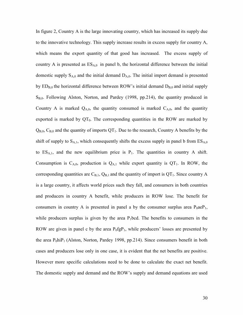
Figure 2: Research benefits, size, and distribution due to trade (large country
exporter innovates, no technology spillover)
a) Country A: Large country b) Excess supply, demand c) ROW production, (innovator) and trade consumption and trade Price Price Price ESA,0 SB,0 SA,0 a SA,1 k ESA,1 h f P0 e P0 P0 i P1 b P1 P1 g d c m DB,0 EDB,0 QT0 DA,0 QT0
QT1 QT1
0 CA,0 CA,1 QA,0 QA,1 QT0 QT1 QB,0 QB,1 CB0 CB,1 Country A Quantity Traded Quantity ROW Quantity
Source: Alston, Norton, and Pardey (1998) p.215
30
In figure 2, Country A is the large innovating country, which has increased its supply due
to the innovative technology. This supply increase results in excess supply for country A,
which means the export quantity of that good has increased. The excess supply of
country A is presented as ESA,0 in panel b, the horizontal difference between the initial
domestic supply SA,0 and the initial demand DA,0. The initial import demand is presented
by EDB,0 the horizontal difference between ROW’s initial demand DB,0 and initial supply
SB,0. Following Alston, Norton, and Pardey (1998, pp.214), the quantity produced in
Country A is marked QA,0, the quantity consumed is marked CA,0, and the quantity
exported is marked by QT0. The corresponding quantities in the ROW are marked by
QB,0, CB,0 and the quantity of imports QT1. Due to the research, Country A benefits by the
shift of supply to SA,1, which consequently shifts the excess supply in panel b from ESA,0
to ESA,1, and the new equilibrium price is P1. The quantities in country A shift.
Consumption is CA,0, production is QA,1 while export quantity is QT1. In ROW, the
corresponding quantities are CB,1, QB,1 and the quantity of import is QT1. Since country A
is a large country, it affects world prices such they fall, and consumers in both countries
and producers in country A benefit, while producers in ROW lose. The benefit for
consumers in country A is presented in panel a by the consumer surplus area P0aeP1,
while producers surplus is given by the area P1bcd. The benefits to consumers in the
ROW are given in panel c by the area P0fgP1, while producers’ losses are presented by
the area P0hiP1 (Alston, Norton, Pardey 1998, pp.214). Since consumers benefit in both
cases and producers lose only in one case, it is evident that the net benefits are positive.
However more specific calculations need to be done to calculate the exact net benefit.
The domestic supply and demand and the ROW’s supply and demand equations are used
31
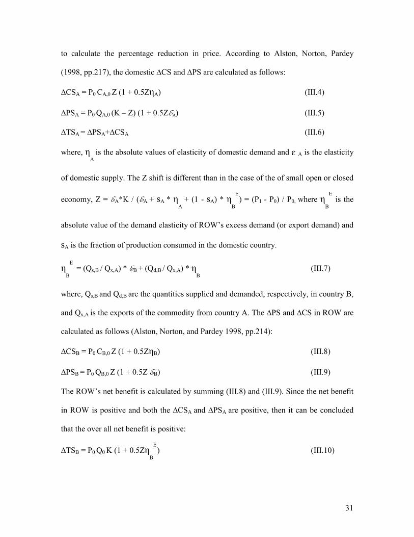
to calculate the percentage reduction in price. According to Alston, Norton, Pardey
(1998, pp.217), the domestic ∆CS and ∆PS are calculated as follows:
∆CSA = P0 CA,0 Z (1 + 0.5ZηA) (III.4)
∆PSA = P0 QA,0 (K – Z) (1 + 0.5ZEA) (III.5)
∆TSA = ∆PSA+∆CSA (III.6)
where, ηA
is the absolute values of elasticity of domestic demand and A is the elasticity
of domestic supply. The Z shift is different than in the case of the of small open or closed
economy, Z = EA*K / (EA + sA * ηA
+ (1 - sA) * ηB
E
) = (P1 - P0) / P0, where ηB
E
is the
absolute value of the demand elasticity of ROW’s excess demand (or export demand) and
sA is the fraction of production consumed in the domestic country.
ηB
E
= (Qs,B / Qx,A) * EB + (Qd,B / Qx,A) * ηB
(III.7)
where, Qs,B and Qd,B are the quantities supplied and demanded, respectively, in country B,
and Qx,A is the exports of the commodity from country A. The ∆PS and ∆CS in ROW are
calculated as follows (Alston, Norton, and Pardey 1998, pp.214):
∆CSB = P0 CB,0 Z (1 + 0.5ZηB) (III.8)
∆PSB = P0 QB,0 Z (1 + 0.5Z EB) (III.9)
The ROW’s net benefit is calculated by summing (III.8) and (III.9). Since the net benefit
in ROW is positive and both the ∆CSA and ∆PSA are positive, then it can be concluded
that the over all net benefit is positive:
∆TSB = P0 Q0 K (1 + 0.5ZηB
E
) (III.10)
ɛ

32
The large exporting country with no technology spillover framework was used to
calculate the consumer and producer surplus in Ecuador, in chapter IV section II. The
formulas explained above were imputed in an Excel spreadsheet after obtaining and
imputing other required data such as prices, quantities, elasticites etc., which produced
the producer and consumer surplus dollar amounts.
If the innovative country is the importing country, in the case above that would be ROW,
and then Figure 2 would look different as well as the ∆PS and ∆CS. If there is a
technology spillover then the outcome will also be different. Figure 3 presents a large
innovative exporter country and the effects of the spillover. This case is important
because it shows the effects of the technology spillover to both countries which affects
the consumer and producer surplus values.
Figure 3: Research benefits size and distribution due to trade (large country
exporter innovates, with technology spillover)
a) Country A: Large country b) Excess supply, demand c) ROW production, (innovator) and trade consumption and trade Price Price Price SB,0 ESA,0 SB,1 SA,0 P0 a P0 ESA,1 h f -------- e SA,1 P1 P0 i P2 b P1 g D c EDB,0 DB,0 EDB,1 k QT0 j DA,0 QT0
QT1 QT1
0 CA,0 CA,1 QA,0 QA,1 QT0 QT1 QB,0 QB,1 CB0 CB,1 Country A Quantity Traded Quantity ROW Quantity
Source: Alston, Norton, and Pardey (1998) p.220
33
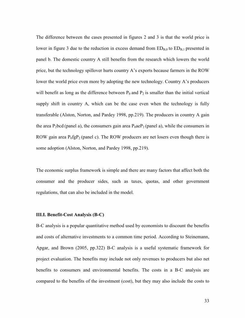
The difference between the cases presented in figures 2 and 3 is that the world price is
lower in figure 3 due to the reduction in excess demand from EDB,0 to EDB,1 presented in
panel b. The domestic country A still benefits from the research which lowers the world
price, but the technology spillover hurts country A’s exports because farmers in the ROW
lower the world price even more by adopting the new technology. Country A’s producers
will benefit as long as the difference between P0 and P2 is smaller than the initial vertical
supply shift in country A, which can be the case even when the technology is fully
transferable (Alston, Norton, and Pardey 1998, pp.219). The producers in country A gain
the area P2bcd (panel a), the consumers gain area P0aeP2 (panel a), while the consumers in
ROW gain area P0fgP2 (panel c). The ROW producers are net losers even though there is
some adoption (Alston, Norton, and Pardey 1998, pp.219).
The economic surplus framework is simple and there are many factors that affect both the
consumer and the producer sides, such as taxes, quotas, and other government
regulations, that can also be included in the model.
III.I. Benefit-Cost Analysis (B-C)
B-C analysis is a popular quantitative method used by economists to discount the benefits
and costs of alternative investments to a common time period. According to Steinemann,
Apgar, and Brown (2005, pp.322) B-C analysis is a useful systematic framework for
project evaluation. The benefits may include not only revenues to producers but also net
benefits to consumers and environmental benefits. The costs in a B-C analysis are
compared to the benefits of the investment (cost), but they may also include the costs to

34
the environment which include emissions, environmental degradation, loss of natural
resources, effects on human health etc. Measuring the benefits and costs to the
environment is difficult and people tend to overlook and undervalue them. There are few
different B-C methods such as net present value (NPV), benefit-cost ratio, internal rate of
return (IRR) etc. In this section the NPV, B-C ratio and the IRR method are presented
and explained in more details because these were used as a part of the economic surplus
analysis in all three sections of chapter IV.
In order to evaluate the benefits and costs, they need to be placed in equivalent terms
over time. The net present value (NPV) is one method used to discount benefits and costs
to a present value (Steinemann, Apgar, and Brown 2005, pp.335).
n n
NPV = [ Σ Bt ] – [ Σ Ct ]
t=0 (1 + r )t t=0 (1 + r )t (III.11)
or
NPV = Σ BPV - Σ CPV (III.12)
where,
t = the time period
r = the discount rate
n = the life of the project
Bt = the benefits in time period t
Ct = the costs in time period t
Σ BPV = the sum of all benefits in present value terms
Σ CPV = the sum of all costs in present value terms
35
(Steinemann, Apgar, Brown 2005, pp.335).
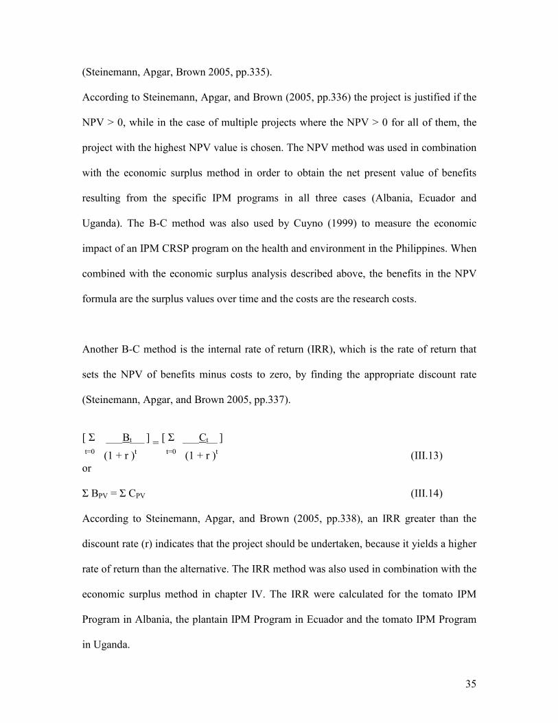
According to Steinemann, Apgar, and Brown (2005, pp.336) the project is justified if the
NPV > 0, while in the case of multiple projects where the NPV > 0 for all of them, the
project with the highest NPV value is chosen. The NPV method was used in combination
with the economic surplus method in order to obtain the net present value of benefits
resulting from the specific IPM programs in all three cases (Albania, Ecuador and
Uganda). The B-C method was also used by Cuyno (1999) to measure the economic
impact of an IPM CRSP program on the health and environment in the Philippines. When
combined with the economic surplus analysis described above, the benefits in the NPV
formula are the surplus values over time and the costs are the research costs.
Another B-C method is the internal rate of return (IRR), which is the rate of return that
sets the NPV of benefits minus costs to zero, by finding the appropriate discount rate
(Steinemann, Apgar, and Brown 2005, pp.337).
[ Σ Bt ] =
[ Σ Ct ]
t=0 (1 + r )t t=0 (1 + r )t (III.13) or
Σ BPV = Σ CPV (III.14)
According to Steinemann, Apgar, and Brown (2005, pp.338), an IRR greater than the
discount rate (r) indicates that the project should be undertaken, because it yields a higher
rate of return than the alternative. The IRR method was also used in combination with the
economic surplus method in chapter IV. The IRR were calculated for the tomato IPM
Program in Albania, the plantain IPM Program in Ecuador and the tomato IPM Program
in Uganda.

36
III.II. Budgeting
Budgets are used in IPM CRSP impact studies to summarize the benefits and costs per
hectare and these estimates are then used in the economic surplus analysis. Daku (2002)
used budgets to summarize the expenses for each experiment and the costs and returns
per acre to produce olives. An enterprise budget includes the value of output and cost of
all inputs devoted to producing one kind of crop or livestock. The enterprise budget
provides information about the profitability of each enterprise relative to the resources
used, it also provides information about relative efficiency of various enterprises (Brown
1979). According to Daku (2002), an enterprise budget summarizes the costs and
projected returns for a single enterprise, it also includes gross returns and variable and
fixed costs. Each enterprise budget is customized to the specific crop and area setting, but
it contains the same main parts.
Another type of budget is a partial budget. According to Brown (1979), the partial budget
consists of four basic items:
Costs Benefits
a) New costs c) Costs saved
b) Revenue forgone d) New revenue
If (c) + (d) > (a) + (b) the change is profitable, given that it is a feasible change.
According to Daku (2002) partial budgets can be developed for each IPM practice, which
will help indentify the cost and revenue items that will change with the implementation of
the new IPM practices. Daku (2002) points out that the partial budget is a partial
application of marginal analysis.
37
Chapter IV. Results of the Additional Analysis of IPM CRSP Impacts
The IPM CRSP studies included in Chapter II were tailored to a specific country, crop,
and/or experiment. In an attempt to include more recent impact analysis, a request was
sent to each IPM CRSP site chair asking them to nominate additional IPM technologies
for evaluation in their sites. This chapter includes additional economic surplus analyses
that were conducted based on the responses received from Albania, Ecuador and Uganda.
Scientist-questionnaires were sent to IPM CRSP site coordinators in: East Africa, West
Africa, Southeast Asia, East Asia, Central Asia, Latin America and Eastern Europe. Each
site that responded compiled their scientist responses and filled out an aggregate scientist-
questionnaire for a specific crop, so one response per site was received. A sample
questionnaire is presented in Appendix A. After receiving the responses, an economic
surplus analysis was conducted for each crop/technology. The appropriate model was
decided upon with respect to the type of market for that product (closed economy, small
open economy, or large open economy). The choice of the appropriate economic surplus
model is affected by the country’s ability to affect world prices. After that the appropriate
data from each questionnaire was entered in an Excel spreadsheet, the information on
prices, quantities produced, exports, imports and consumption were found using
FAOSTAT. The benefit time period was different for every project, depending on when
the project started but the usual research timeframe used was 15 years. Therefore the data
for each project was spread out over a 15 year time period. The elasticity of supply is
problematic if linear supply and demand curves are used because when the function is
inelastic at the equilibrium a negative intercept at the price axis is implied. Therefore
various authors have criticized the use of linear supply curves with point elasticity of less
ɛ

38
than one (Alston, Norton, and Pardey 1998, pp.63). To avoid this type of problem and
due to limited information about the actual supply elasticities, the supply elasticity was
assumed to be 1 in the cases that were examined. A supply elasticity of 1 was also used in
most of the previous studies for same products and countries. The demand elasticities
were also obtained from previous studies.
A full list of the variables used in the economic surplus analyses as well as explanations
about each variable are available in Appendix B. Using the formulas discussed in the
chapter III, the total economic surplus was calculated first and than the NPV of the
benefits was calculated, using a 5% discount rate.
IV.I. Tomato IPM Program in Albania
According to the Food and Agriculture Organization (FAO), tomatoes are the fourth most
important agricultural product in Albania. In 2006, Albania produced 164,853 metric tons
of tomatoes, the area harvested was 7,385 ha, and the yield per hectare was 22,323 kg/ha.
On average from 2000 to 2005 Albania imported 6,121 metric tons of tomatoes and
exported approximately 127 metric tons of tomatoes. Due to the small quantities of
exports and imports Albania can be considered a closed economy with respect to the
tomato market. The IPM CRSP has been working with Albanian producers to improve
their tomato production practices. In order to manage the root-knot nematode
(Meloidoyne inconita) problem, the IPM practice of soil solarization was used. The
solarization process includes covering the soil with plastic-sheet after harvest and before
planting the new seeds. This process destroys the pathogens in the soil that later can
39
cause the root-knot nematode problem. According to Albanian scientists, a yield
improvement of 50-200% occurred with IPM use compared to the untreated control, and
50% as compared to previous practice. A 50% yield change was assumed in the
economic surplus analysis. The percent change in cost per hectare used in the economic
surplus analysis was calculated using the data provided by the scientists. The cost change
was estimated to be –0.39%. The scientists suggested that maximum adoption rate of 65-
70% will be achieved by year 2014, which sounds optimistic. Past experience with
adoption of improved practices suggests that a more reasonable adoption estimate would
be about 25%. Currently 1.5% of the farmers have adopted the IPM practice and there are
only 4ha of tomatoes grown under the IPM practice. A maximum adoption rate of 25%
was assumed in our analysis. The price of tomatoes per ton was estimated by using
average prices per ton of tomatoes for the years 2000-2002-2004 which were obtained
from the FAOSTAT (2008). The quantities of tomatoes produced were obtained only for
the green-houses and low-tunnels production in Albania because the scientists who
responded to the scientist-survey indicated that they were answering the questions
regarding green-house tomato production. The average quantity of tomatoes produced in
green-houses and low-tunnels was averaged for each and than added together for the
same time period as the prices. The average price was $308 per metric ton (FAOSTAT,
2008) and the average quantity was estimated to be 26,969 metric tons (Matotan Z., and
Abacus, 2009). Varying the price and the quantity per year would not change the results
since the annual variation is not large, therefore using average prices and quantities is
recommended. The elasticity of supply was assumed to be 1, due to the factors described
in the previous section. An additional factor supporting the assumption was the fact that

40
tomato producers can divert land into tomato production relatively quickly. The elasticity
of demand for tomatoes in Albania was -0.5 (Rickard and Sumner 2006). The economic
surplus analysis was conducted for the time period 2007 to 2022. The costs reported by
the Albanian scientists were for the years from 2007 to 2014, but the costs reported in
2014 were carried over until year 2022. The consumer and producer surplus analysis
yielded positive values for all years. The benefits and costs of the IPM practice were
discounted at 5% giving a NPV of approximately USD $8 million2 over 15 years. The
IRR was incalculable due to the large value of the benefits and very small value of the
costs.
Due to the uncertainty of the assumptions, a sensitivity analysis was conducted. Scientists
reported that the adoption rate will reach 65-70% by 2014. Consequently the adoption
rates were changed in such a way that the highest value was 70% as the scientists had
suggested initially. This change in the adoption rate increased the NPV to about USD $23
million3 for the 15 year period.
In the second sensitivity analysis, the percent change in cost per hectare was changed to
25%. The responses received in the scientist-questionnaire regarding the cost per hectare
may have been too low because scientists may have misinterpreted the question.
Knowledge and practice suggest that -0.39% change in cost per hectare is too low, and
that is why in the sensitivity analysis a 25% cost per hectare change was used. Another
reason for the cost uncertainty may be the fact that only 4 hectares of tomato are currently
2 Refer to Appendix C for the economic surplus analysis table 3 Refer to Appendix D for the sensitivity analysis table

41
grown under the IPM practice, so there is little commercial experience with it, as farmers
only started adopting the IPM practice in 2007. Changing the percent change in cost per
hectare to 25% resulted in a decrease of the NVP to about USD $5 million over the 15
year period, with a 5% discount rate.
The following table summarizes the NPV of benefits produced by the economic surplus
analysis of tomatoes in Albania.
Table 2: Summary of the results from the economics surplus analysis and sensitivity
analysis for tomato IPM in Albania
6VP
Original, max adoption
rate = 25% $8,358,811.98
Sensitivity Analysis
Case 1 : Adoption rate
change = 70% $22,714,675.68
Case 2: Percent change in
cost per hectare = 25% $5,498,633.82
IV.II. Plantain IPM Program in Ecuador
For the time period 2001-2007, Ecuador was the third largest producer of plantain in
South America (FAOSTAT, 2008a). According to the FAOSTAT (2008a), in 2006
Ecuador was the largest South American exporter of plantain, while in 2005 Ecuador was
the second largest exporter after Columbia. In 2006 Ecuador exported 166,688 metric
tons of plantain, which is approximately 30% of the world plantain exports. In 2006,
42
South America exported 365,787 metric tons of plantain, which was approximately 67%
of the world’s plantain exports (FAOSTAT, 2008a). This trade implies that the
appropriate model for the economic surplus analysis is a large exporting economy model.
According to the Ecuadorian scientists, the IPM practice used is referred to as IPM
management which includes sanitization of the crop, fertilization and population (of
plantains) regulation, cultural practices and biological control. The scientists estimated
the percent yield change per hectare to be 100% for farmers who adopt the complete set
of IPM practices. The percent change in cost per hectare was estimated to be
approximately 37%. The scientists also indicated that with IPM, the use of pesticides
such as gliphosate and carbofuran is reduced. The plantain IPM project began in 1999
and thus far 5000 out of available 45,000 hectares of plantain are currently grown under
the IPM practice suggested by the IPM CRSP, which is 11% of the available hectares.
The scientists believe that so far 0.2% of the farmers have adopted the IPM practice but
the adoption had started in the 4th year (2003). The percentage of hectares used did not
equal the number of farmers who adopted the technology because of the uneven per
farmer acre distribution. The maximum adoption was expected to reach 5% of the
farmers, and was expected to be achieved in 5 years. The supply elasticity for plantain
was assumed to be 1 based on the argument made by Alston, Norton, and Pardey (1998)
in the beginning of this chapter. According to Baez (2004) the elasticity of demand for
plantain was -0.3, indicating that plantain is a staple food in Ecuador. The large open
economy model leads to the use of an excess-demand-supply framework. The calculation
of ηB
E
- absolute value of the demand elasticity of ROW’s excess demand (or export
demand) - requires the supply and demand elasticities for the ROW. The ROW’s plantain

43
elasticities of supply and demand are expected to be more elastic than the ones in the
domestic country because the elasticities in the ROW are aggregated excess demand and
supply of the rest of the trading countries. The ROW’s plantain elasticity of supply ηB
was assumed also to be 1, while ROW’s demand elasticity was assumed to be -0.6
considering the information available for bananas (Baez 2004). Using the formula for the
absolute value of the demand elasticity of ROW’s excess demand (or export demand) ηB
E
which was defined in section III formula III.7 yields a ηB
E
of 167.89. The price and
quantity produced used in the economic surplus analysis were averaged for the period
from 2001 to 2003 and were USD $61 and 714,094 metric tons, respectively (FAO STAT
2008a). Since the large open economy model was used, another piece of information was
needed, the quantities consumed domestically. These were obtained from FAO STAT
(2008a), the consumption quantities were also averaged from 2001 to 2003. The average
quantity consumed in Ecuador was 467,722 metric tons. The research and dissemination
costs reported by the scientists are for the time period 1999-2006, however since no
information was available for the costs after year 2006 which were $4,000. The costs
from year 2006 were carried over until year 2013. Including these costs in the economic
surplus analysis did not affect the results significantly, since the benefits from adoption of
the IPM practices were much higher than the costs. Using the formulas from Chapter III
regarding the open economy model, the economic surplus analysis resulted in a NPV of
benefits over the 15 year period, discounted at 5%, of approximately USD $7 million4
and the IRR was estimated to be 110%.
4 The economic surplus analysis table for Plantain in Ecuador is in Appendix E
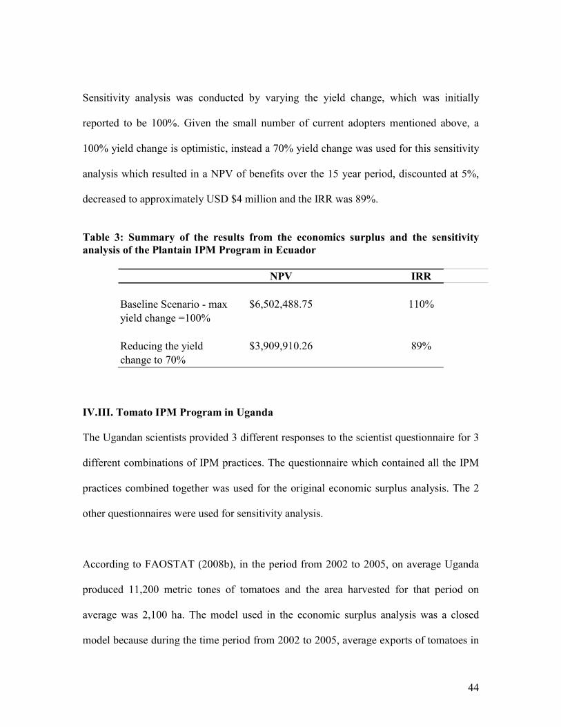
44
Sensitivity analysis was conducted by varying the yield change, which was initially
reported to be 100%. Given the small number of current adopters mentioned above, a
100% yield change is optimistic, instead a 70% yield change was used for this sensitivity
analysis which resulted in a NPV of benefits over the 15 year period, discounted at 5%,
decreased to approximately USD $4 million and the IRR was 89%.
Table 3: Summary of the results from the economics surplus and the sensitivity
analysis of the Plantain IPM Program in Ecuador
6PV IRR
$6,502,488.75 110%
$3,909,910.26 89%
Baseline Scenario - max
yield change =100%
Reducing the yield
change to 70%
IV.III. Tomato IPM Program in Uganda
The Ugandan scientists provided 3 different responses to the scientist questionnaire for 3
different combinations of IPM practices. The questionnaire which contained all the IPM
practices combined together was used for the original economic surplus analysis. The 2
other questionnaires were used for sensitivity analysis.
According to FAOSTAT (2008b), in the period from 2002 to 2005, on average Uganda
produced 11,200 metric tones of tomatoes and the area harvested for that period on
average was 2,100 ha. The model used in the economic surplus analysis was a closed
model because during the time period from 2002 to 2005, average exports of tomatoes in

45
Uganda were 19 metric tones and average imports were 15.5 metric tones, which in both
cases is a very small amount for tomato to be considered as an important export crop. The
scientists reported that the IPM practices applied on tomato production were a
combination of staking, mulching, minimum pesticides, raisedbeds, and resistant variety.
The percent yield change per hectare was reported to be 42%. According to the data
provided by the scientists the percent change in cost per hectare was estimated to be 1%.
The development of the IPM practices started in 2002, but the dissemination process
began in 2004. Farmers started adopting the IPM practices in 2005, and currently 5% of
all tomato growers have adopted the IPM practices. The maximum adoption is expected
to be achieved by 2016, and according to the scientists the maximum adoption is
expected to reach 70%. Knowledge and experience suggest that 70% adoption is an over-
optimistic assumption, as in most cases the maximum adoption reaches approximately
25%. The 25% adoption rate was used in the baseline scenario analysis. The costs
provided by the scientists are for the years 2002 to 2008. Since there is no information
about the costs after 2008, the 2008 costs were carried out until 2016. Due to the
unavailability of price data for tomatoes in Uganda, the price used in the economic
surplus analysis was generated using tomato prices from nearby countries for the 2002-
2005 period. The average price was estimated by averaging the prices in each of the four
counties: Ethiopia, Kenya, Malawi and Mozambique for each year and then the averages
from 2002, 2003, 2004 and 2005 were averaged again. The price obtained was
approximately $195 per metric ton of tomatoes. Due to the lack of previous studies and
according to the argument made by Alston, Norton, and Pardey (1998) in at the beginning
of this chapter IV, the elasticity of supply was assumed to be 1. The elasticity of demand
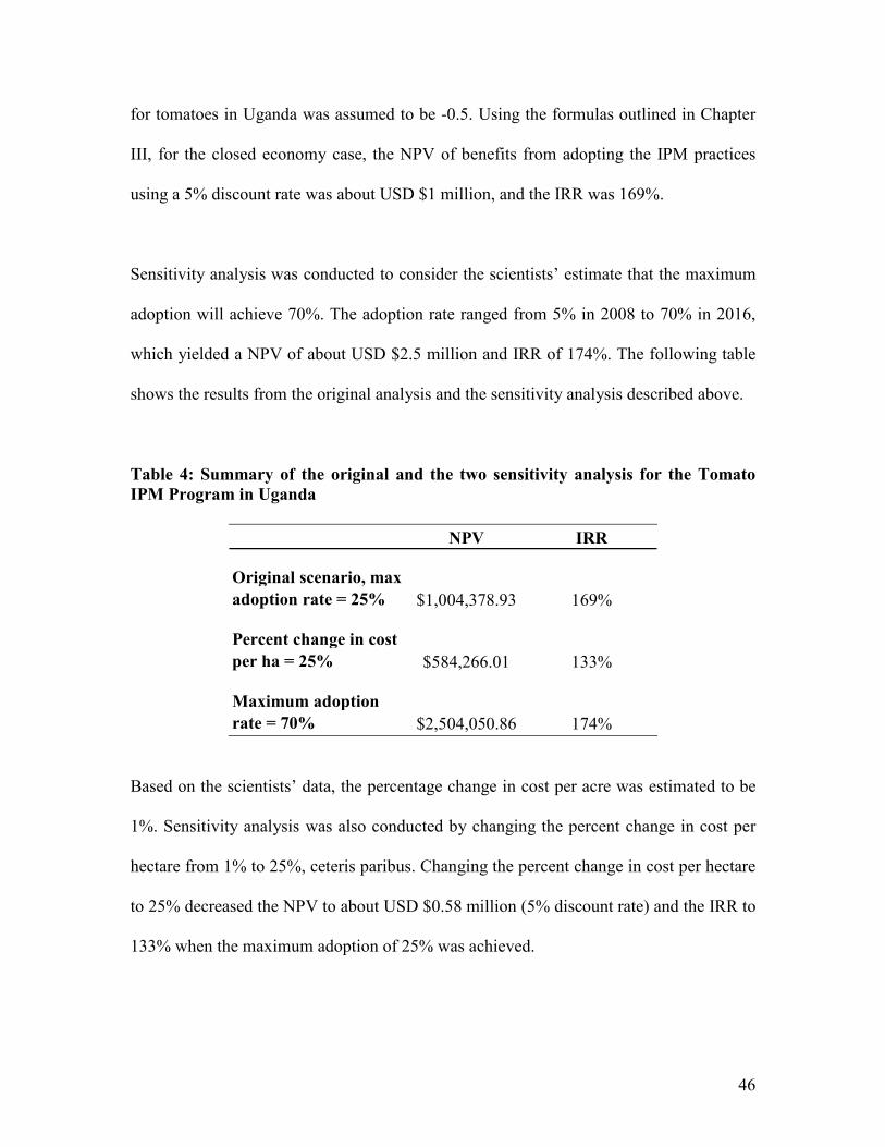
46
for tomatoes in Uganda was assumed to be -0.5. Using the formulas outlined in Chapter
III, for the closed economy case, the NPV of benefits from adopting the IPM practices
using a 5% discount rate was about USD $1 million, and the IRR was 169%.
Sensitivity analysis was conducted to consider the scientists’ estimate that the maximum
adoption will achieve 70%. The adoption rate ranged from 5% in 2008 to 70% in 2016,
which yielded a NPV of about USD $2.5 million and IRR of 174%. The following table
shows the results from the original analysis and the sensitivity analysis described above.
Table 4: Summary of the original and the two sensitivity analysis for the Tomato
IPM Program in Uganda
6PV IRR
Original scenario, max
adoption rate = 25% $1,004,378.93 169%
Percent change in cost
per ha = 25% $584,266.01 133%
Maximum adoption
rate = 70% $2,504,050.86 174%
Based on the scientists’ data, the percentage change in cost per acre was estimated to be
1%. Sensitivity analysis was also conducted by changing the percent change in cost per
hectare from 1% to 25%, ceteris paribus. Changing the percent change in cost per hectare
to 25% decreased the NPV to about USD $0.58 million (5% discount rate) and the IRR to
133% when the maximum adoption of 25% was achieved.

47
The following sensitivity analyses (case 1 and 2) were based on the 2 other5
questionnaires.
Case 1: The scientists reported the combination of practices to be: mulching, minimum
pesticides, raisedbeds and resistant variety. The yield change in this case was reported to
be 25%, instead of the 42% in the initial (original) analysis. The percent change in cost
per hectare also changed from 1%, the new percent change in cost per acre was estimated
to be -0.5%. The maximum adoption was again expected to be 70%. However, as in the
original analysis a 25% adoption rate was used, based on knowledge and previous
experience. The costs for development and dissemination changed per year but the same
procedure was applied in which the 2008 costs were carried out until 2016. The new
analysis at 5% discount rate, yielded NPV of approximately USD $0.03 million and IRR
was 43% when adoption reaches a maximum of 25%.
Case 2: The combination of IPM practices in this case was: staking, minimum pesticides,
raisedbeds and MT56. The new combination resulted in a 30% yield change and a new
percent change in cost per hectare. The change in cost per hectare went from 1% in the
original scenario to 0.25%. The maximum adoption was again expected to reach 70% but
based on the previously mentioned assumptions a 25% adoption rate was used. The
development and dissemination costs changed again but the same practice was applied,
the costs from year 2008 were carried to 2016. The new changes resulted in a new NPV
of approximately $0.8 million (at 5% discount rate) and IRR of 270% when the adoption
5 For more information please refer to the beginning of section: Tomato IPM Program in Uganda.

48
rate was maximum 25%. The table below is used to summarize the effects from case 1
and case 2:
Table 5: Summary of the case 1 and case 2 economic surplus analyses conducted in
the case of the Tomato IPM Program in Uganda
6PV IRR
Maximum Adoption ≤ 25%
Case 11
$29,721.91 43%
Case 22
837,665.57 270%
1 The analysis is based on the scientist-questionnaire contatining the following
mix of IPM practices: mulching, minimum pesticides, raisedbeds and resistant
variety (including MT56).
2 The analysis is based on the scientist-questionnaire contatining the following
mix of IPM practices: staking, minimum pesticides, raisedbeds and MT56.

49
Chapter V. Factors Determining Adoption of IPM Technologies in Bangladesh
An adoption analysis is necessary to describe and measure the adoption of IPM
technologies, which can provide important policy information that can lead to
improvement of farmers’ lives. The objective of chapter V is to determine the factors that
affect adoption of IPM technologies in Bangladesh, using survey data from four districts.
The chapter includes the following sub-sections: basic background information about
Bangladesh, technology adoption discussion and literature review, description the
econometric model, description of the variables in the econometric model, and results and
conclusions.
V.I. Basic Background Information
Bangladesh is located in the southern part of Asia. It is bordered by India, Myanmar and
the Bay of Bengal. Bangladesh is one of the world’s most populous nations with 158.6
million citizens. In 2007 the gross domestic product (GDP) was reported to be $67.7
billion dollars, while GPD per capita was approximately USD $426, the average annual
GDP growth was reported to be 6.5% (World Bank 2008). Life expectancy at birth in
2007 in Bangladesh was 64 years, and the literacy rate was 47% (World Bank 2008). In
2007, the agriculture sector was estimated to be 18.9% of GDP, and the agricultural
annual growth was estimated to be 3.2%. Rakshit (2008) describes Bangladesh as an
overpopulated country, heavily dependent on agriculture, with high seasonal
unemployment among farm workers, which leads to a generally low standard of living in
most areas. According to the US Department of State (2008), 62.3% of the work force in
Bangladesh which is about 60.3 million people, works in agricultural jobs. Numerous
50
world organizations have been working to improve the lives of people in Bangladesh,
including the IPM CRSP. There are various ways to improve farmers’ lives in
Bangladesh using IPM CRSP techniques and approaches, such as developing resistant
varieties, educating farmers though FFS’s, etc. Impact analyses regarding different
agriculture related aspects in Bangladesh have been conducted by Rakshit (2008),
Victoria (2007), Mishra (2003), Alponi (2003), Debass (2000) and others. One way to
improve the lives of farmers in most developing countries is through adoption of
innovative agricultural technologies. Considering the fact that the majority of the
population in LDCs depends on agricultural production, new technologies may provide an
opportunity to increase production and income significantly (Feder, Just, and Zilberman 1985).
V.II. Technology adoption discussion and literature review of IPM adoption
Technology adoption has been studied extensively over the years, and different authors
have defined technology differently. In general a new technology can be defined as a new
way of production. New technologies are usually associated with risk, uncertainty and
distrust in the minds of farmers, which are obstacles to adoption. According to Feder, Just
and Zilberman (1985), other constraints to adoption of innovative technologies are the
“lack of credit, limited access to information, inadequate farm size, inadequate incentives
associated with farm tenure arrangements, insufficient human capital, absence of
equipment to relieve labor shortages (thus preventing timeliness of operations), chaotic
supply of complementary inputs (such as seed, chemicals, and water), and inappropriate
transportation infrastructure.” Economists often associate technology improvement with
increase of productivity, decrease of labor and increase of leisure. In agriculture,

51
technologies have been introduced as packages containing several components such high
yield varieties (HYV), fertilizers and corresponding land preparation (Feder, Just and
Zilberman 1985).
Feder, Just, and Zilberman (1985) also point out that before defining adoption it is
important to distinguish between individual (farm-level) and aggregate adoption, defining
final adoption at the level of the individual farmer as the “degree of use of a new
technology in long-run equilibrium when the farmer has full information about the new
technology and its potential” while the aggregate level of adoption is measured by the
aggregate use of technology within a specific geographic area.
Mauceri (2004) analyzed the adoption of IPM technologies in the case of potato
production in Carchi, Ecuador, using an ordered probit model. The variables used in the
adoption analysis were: age, farm size, education, family size, number of family members
14 years and older, landholdings per capita, pesticide health impact on the farmer and the
family, FFS attendance, information access though field days, pamphlets and exposure to
FFS participants. The study found that, apart from information factors the only socio-
economic factor that was significant was household size, and it impacted IPM adoption
negatively. The data were obtained through a farmers’ survey, however the sample was
non-random and small which limited the analysis. Mauceri (2004) also looked at the cost-
benefit of various information diffusion methods, and the extent of adoption in addition
to analyzing the determinants and constraints to adoption. The study found that FFSs are

52
cost-effective and require little if any additional capital but are not the most cost effective
dissemination techniques. (Mauceri 2004)
Bonabana-Wabi (2002) analyzed the factors affecting adoption of IPM technologies in
the Kumi district, Eastern Uganda. In addition, she also analyzed the relative contribution
of each factor affecting IPM adoption and the level of adoption of eight IPM
technologies. The study analyzed the adoption of eight IPM technologies on cowpea,
sorghum and groundnuts in Kumi. Low adoption (< 25%) was found with five
technologies, while high adoption (> 75%) was found with three technologies. Using
univariate and multivariate logit models, the eight practices were analyzed and it was
found that information access positively affects adoption of IPM technologies. It was also
found that social factors do not affect sorghum technology adoption, except celosia (an
exotic legume that reduces striga) which was positively affected, and in that case males
were more likely to adopt the technique of intercropping sorgum with celosia than
females. Farm experience was found to positively affect timely planting of cowpea. Some
of the significant economic factors found by the study to affect adoption were the farm
labor availability and disease incidence, which affect adoption of celosia and other Striga
chasers, negatively (Striga chasers such Celosia reduce Striga emergence in sorghum). In
the sorghum crop rotation model, adoption of crop rotation was found to reduce weed
problems. In the cowpea case, it was found that intercropping was used as both a land-
saving technology and a pest management strategy. (Bonabana-Wabbi 2002)

53
De Souza Filho, Young, and Burton (1999) analyzed the factors influencing adoption of
sustainable agricultural technologies in Espitito Santo, Brasil, using an alternative
approach called discrete econometric framework (duration analysis).The study found that
access to information (through membership in farmers organizations, NGO presentations,
pamphlets etc.) positively affects adoption, and also increases the awareness of negative
effects due to pesticide use. In this study farm size was found to affect adoption
negatively. It was also found that an increase in output prices and rural wages relative to
prices of external inputs decreases the speed of diffusion of sustainable agricultural
technologies (De Souza Filho, Young, and Burton 1999).
Another study by Chaves and Riley (2001) determined the factors influencing integrated
pest management adoption to combat coffee berry borer on Colombian farms. The factors
affecting adoption were said to be social, economic, environmental and institutional. A
logistic regression analysis was used to determine the impact of different factors, but first
some standard non-linear curves were fitted and contrasted to the uptake data for each of
the four chosen IPM recommendations for coffee berry borer control. Since the different
factors were analyzed at different times upon the uptake of the recommendations singly
and in combination, there were different scenarios. The study found education to be an
important influential factor positively affecting adoption under all scenarios, while the
size of coffee plots was found to be important in all cases in most of the years, and wealth
was also found to be an influential factor affecting adoption.
54
V. III. The econometric model: an ordered probit
The dependent variable in the following adoption analysis can take four values 1, 2, 3 and
4, indicating different levels of adoption. Due to the ordered nature of the dependent
variable the model used was an ordered probit model. The ordinary least squares (OLS)
models are not the adequate estimators for these types of cases because they are not
necessarily consistent in the probability discrete choice framework. The OLS estimator
measures the change in the dependent variable given one unit change in the independent
variable and could offer results that are negative or exceed the maximum value. The
ordered probit model ensures a result that lies within the interval of interest (Wooldridge
2006). The ordered probit model was also used by Mauceri (2004), while Feder and
Umali (1993) also suggested the use of the logit/probit models for technology adoption
analysis. The ordered probit requires a dependent variable that, as suggested by the name,
is ordered, which means that the assigned values are no longer arbitrary but are rather
ordered responses taking on values {0, 1, 2….J} (Wooldridge 2002).
In their study, Mullen, Norton and Reaves (1997) pointed out that adoption can be
defined by level, while Mauceri (2004) used the level defined adoption approach (ordered
probit model) in the adoption analysis.
The dependent variable in this analysis, was also defined by levels: none, low, medium
and high which correspond respectively to 1, 2, 3, and 4.

55
1 - indicated no adoption, meaning that none of the IPM practices were used by that
particular farmer.
2 - indicated low adoption, meaning that one of the IPM practices was adopted by the
particular farmer.
3 – indicated medium adoption, meaning that two IPM practices were adopted.
4 - indicated high adoption, meaning that three of more practices were adopted by the
particular farmer.
The dependent variable was created by looking at seven different variables, which
referred to the usage of IPM practices, and using the above guidelines. The practices used
to define the dependent variable were: resistant variety, biological control, burning
sawdust, poultry refuse, mustard/neem oil cake, mashed sweet gourd traps and
pheromones. The sawdust, poultry refuse and mustard/neem oil cake are soil amendments
(bedding). Except for the resistant variety and biological control, each other practice was
considered as a separate dummy variable. The biological control and resistant variety
belonged in one variable regarding the control of the most important pest to that farmer.
There was another category for the second most important pest to the farmers. The
farmers were asked whether they used pesticides, biological control, resistant variety or
other practices, regarding their most important and second most important pest. Finally,
there were seven individual variables: the control of the most important pest (pesticides,
biological control, resistant variety or other practices), the control of the second most
important pest (pesticides, biological control, resistant variety or other practices), burning
sawdust, poultry refuse, mustard/neem oil cake, mashed sweet gourd traps and

56
pheromones. Looking at the seven variables, if the farmer used only one practice a 2 was
registered, which indicated low IPM adoption, if any two practices were used a 3 was
registered, which indicated medium level of IPM adoption etc.
According to Wooldridge (2002, pp.504), a latent variable model can be used to derive
the ordered probit model, where y* is determined by
y* = x β + е, e | x ~ Normal (0,1) (V. 1)
where β is K x 1 and x does not contain a constant.
y = 0 if y* ≤ α1
y = 1 if α1 < y* ≤ α2
(V. 2)
y = J if y* > αJ
where α1 < α2….< αJ are the cut points or threshold parameters. The number of threshold
parameters depends on the number of values taken by y, for instance if the values of y are
0, 1 and 2 than there will be two cut points α1 and α2. In the case of the adoption analysis
of IPM adoption in Bangladesh, y takes on the values 1, 2, 3 and 4, resulting in three cut
points α1, α2 and α3.
Given the standard normal assumption for e, the conditional distribution of y given x can
be derived by calculating each response probability:
P (y = 0 | x) = P ( y* ≤ α1 | x ) = P ( x β + e ≤ α1 | x ) = Φ ( α1 - x β )
P (y = 1 | x) = P (α1 < y* ≤ α2 | x ) = Φ ( α2 - x β ) - Φ ( α1 - x β )
. . .
. . . (V. 3)
. . .
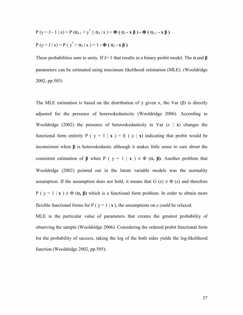
57
P (y = J - 1 | x) = P (αJ-1 < y* ≤ αJ | x ) = Φ ( αJ - x β ) - Φ ( αJ-1 - x β )
P (y = J | x) = P ( y* > αJ | x ) = 1 - Φ ( αJ - x β )
These probabilities sum to unity. If J= 1 that results in a binary probit model. The α and β
parameters can be estimated using maximum likelihood estimation (MLE). (Wooldridge
2002, pp.505)
The MLE estimation is based on the distribution of y given x, the Var (β) is directly
adjusted for the presence of herersokedasticity (Wooldridge 2006). According to
Wooldridge (2002) the presence of heteroskedasticity in Var (e | x) changes the
functional form entirely P ( y = 1 | x ) = E ( y | x) indicating that probit would be
inconsistent when β is heteroskedastic although it makes little sense to care about the
consistent estimation of β when P ( y = 1 | x ) ≠ Φ (α, β). Another problem that
Wooldridge (2002) pointed out in the latent variable models was the normality
assumption. If the assumption does not hold, it means that G (z) ≠ Φ (z) and therefore
P ( y = 1 | x ) ≠ Φ (α, β) which is a functional form problem. In order to obtain more
flexible functional forms for P ( y = 1 | x ), the assumptions on e could be relaxed.
MLE is the particular value of parameters that creates the greatest probability of
observing the sample (Wooldridge 2006). Considering the ordered probit functional form
for the probability of success, taking the log of the both sides yields the log-likelihood
function (Wooldridge 2002, pp.505):
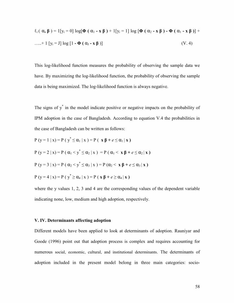
58
ℓi ( α, β ) = 1[yi = 0] log[Φ ( α1 - x β ) + 1[yi = 1] log [Φ ( α2 - x β ) - Φ ( α1 - x β )] +
…..+ 1 [yi = J] log [1 - Φ ( αJ - x β )] (V. 4)
This log-likelihood function measures the probability of observing the sample data we
have. By maximizing the log-likelihood function, the probability of observing the sample
data is being maximized. The log-likelihood function is always negative.
The signs of y* in the model indicate positive or negative impacts on the probability of
IPM adoption in the case of Bangladesh. According to equation V.4 the probabilities in
the case of Bangladesh can be written as follows:
P (y = 1 | x) = P ( y* ≤ α1 | x ) = P ( x β + e ≤ α1 | x )
P (y = 2 | x) = P ( α1 < y* ≤ α2 | x ) = P ( α1 < x β + e ≤ α2 | x )
P (y = 3 | x) = P ( α2 < y* ≤ α3 | x ) = P (α2 < x β + e ≤ α3 | x )
P (y = 4 | x) = P ( y* ≥ α4 | x ) = P ( x β + e ≥ α4 | x )
where the y values 1, 2, 3 and 4 are the corresponding values of the dependent variable
indicating none, low, medium and high adoption, respectively.
V. IV. Determinants affecting adoption
Different models have been applied to look at determinants of adoption. Rauniyar and
Goode (1996) point out that adoption process is complex and requires accounting for
numerous social, economic, cultural, and institutional determinants. The determinants of
adoption included in the present model belong in three main categories: socio-
59
demographic, economic, and institutional characteristics. The same categories were used
by Mauceri (1999) and Wabbi-Bonabana (2002).
The adoption analysis is based on Bangladesh survey data, collected in the summer of
2006 and used by Rakshit (2008) who conducted an IPM impact assessment study of
pheromone adoption for cucurbit crops in Bangladesh. However an adoption analysis was
not conducted. The four districts of Jessore, Comilla, Chittagong and Norsingdi, were
chosen because they are intensive vegetable growing regions (Rakshit 2008). The survey
sample consisted of 300 Bangladeshi farmers, who ranged in age from 14 to 70 years,
with 8 percent below the age of 20, and an average age of approximately 38 years. Eighty
five percent of the farmers reported having experienced (or a family member having
experienced) a health problem due to pesticide use. Also according to the survey data, 17
percent of the farmers were female, all of them in the Norsingdi district. Land holdings
ranged between .23 and 66 acres, with an average of 3.18 acres, and 60% of the farmers
owned less than 2 acres of land. In Bangladesh, land holdings are represented in decimals
(tenth of an acre) instead of acres due to the small size of land holdings. Even though the
survey used the decimal marking system, land holdings were converted to acres for the
purpose of the adoption analysis. Only five farmers reported owning more than 20 acres
of land which for a country as poor as Bangladesh is not very likely so those numbers
were thrown out of the analysis data as an outliers. About 77% of the farmers responded
that they had received IPM training, and 44% of them reported losses greater than 30%
due to annual vegetable yield loss due to pests. The number of working family members
(14 years or older) ranged from 0 to 13 members, with an average of about 3 family
60
members. About 24 % of the farmers reported the number of working members to be
greater than 4. The average level of education was approximately 5 years, ranging from 0
to 16 years. Bangladeshi primary school education is 5 years, but according to the
USAID (2009) it takes Bangladeshi children 6.6 years to complete it. In this sample,
approximately 40% of the surveyed farmers reported having education greater or equal to
7 years, meaning they had at least primary school. According to the reported usage of
IPM practices, about 29 percent of the respondents were high adopters, while 20 percent
were medium adopters. The IPM practices used to define the dependent variable were
discussed in the previous section of this chapter.
i. Category I. Socio-demographic Characteristics
District – Farmer’s district
The variable “district” was a dummy. Each of the four different Bangladeshi districts:
Jessore, Comilla, Chittagong and Norsingdi, was represented by one variable: District1,
District2, District3 and District4, respectively. These distinguished the district to which
each farmer belongs. The coefficients on this variable (District1, District2, District3
and District4) indicated the variation between districts which could be used to increase
adoption and/or improve policy in the low adoption districts. Feder and Slade (1984) used
a binary district variable in the logit analysis of factors affecting the probability of
knowledge and adoption. For the purpose of this adoption analysis the four districts were
converted in four different dummy variables. Each dummy variable corresponds to one
district, however one district had to be dropped because of the dummy variable trap.

61
Age – Farmer’s age
Age is expected to negatively affect adoption. Older and more experienced farmers may
be less likely to experiment with new technologies while younger farmers are less risk
averse and more likely to adopt new techniques. Mauceri (2004) included age in the
ordered probit model, pointing out that younger farmers are still in the process of learning
the best management techniques. Adesina et al. (2000) found age to be negatively related
to adoption of ally cropping. Chaves and Riley (2001) found age to be negatively
correlated and very influential factor in the adoption of IPM for coffee berry borer on
Colombian farms.
Female – Farmer’s Gender (Female=1, Male=0)
Female is a binary variable distinguishing between male and female farmers. Gender
analysis has been an important part of IPM CRSP research. “Yet there are many obstacles
to incorporating women in IPM programs around the world, ranging from traditional
culture to the fact that gender influences access to resources such as land, labor,
education and credit—all important to the adoption of IPM” (IPM CRSP, 2008c).
Mauceri (2004) and Bonabana-Wabbi (2002), both found that the farmer’s gender (male
of female) was not a significant variable affecting technology adoption, in addition
Bonabana-Wabbi (2002) also suggests that the effects of the variable are indeterminate.
Rauniyar and Goode (1996) also found the effects of this variable to be indeterminate.
Educ - Level of farmer’s education

62
Educ is a continuous variable that represent the number of years of education. More
educated farmers were expected to be more open to adoption of innovative technologies,
such IPM technologies. Feder, and Slade (1984) categorized education along with
experience, as a part of human capital, and point out that a higher endowments of human
capital affects productivity positively. Chaves, and Riley (2001), found that higher levels
of education were associated with higher adoption. Another study found that education
was not a significant variable affecting adoption of technologies (Feder and Umali 1993).
A study by Rauniyar and Goode (1996) hypothesized a positive sign for the education
variable based on the fact that higher human capital should increase adoption.
Work - Number of family working members
Work, is a continuous variable which represents the number of working members (14
years and older) in the family. This variable measured the labor availability which is a
factor in adoption (Mauceri 2004). A study by De Souza Filho, Young, and Burton
(1999) found the variable to be significant and positively affecting the adoption of IPM
technologies. Another study however, found that family size was negatively correlated
with adoption in the case of alley farming by farmers in the forest zone of southwest
Cameroon (Adesina et al 2000).
Expr - Farming experience
Exper, is a continuous variable that represents the years of farming experience.
According to Feder and Slade (1984), farm experience along with education could be
represented as human capital which positively impacts adoption. However in this case,
63
experience is expected to negatively affect adoption, because more experienced farmers
may already have picked profitable practices and would be averse toward change.
ii. Category II. Economic Characteristics
FarmInc - The share (low or high) of farm income from total annual income
FarmInc, is included as a dummy variable, which shows the importance of farming for
that particular farmer. It is expected to affect adoption negatively. If the share of farm
income is high (≥ 50%) farmers were expected to be more risk averse and less likely to
try new technologies. Farmers with a low share of farm income (<50%) are expected to
be more open to adopting new technologies in order to increase their returns.
Fland - Total size of Farm Land (including own, rented, sharecropped etc. land)
Fland, is a continuous variable measuring the total land holdings in acres. Mauceri (2004)
used per capita measure of the land size and found that the variable had no significant
impact on adoption while the signs in the different model adaptations were conflicting.
Mauceri (2004) pointed out that the difference in the signs may be due to the nature of
the IPM technology, larger farms are expected to adopt more capital intensive
technologies while smaller farms are expected to adopt more labor intensive
technologies. In another study farm size was found to be negatively correlated with
adoption (De Souza Filho, Young, and Burton 1999).
iii. Category III. Institutional Characteristics

64
Exten – distance (km) to the nearest extension agent.
Exten, is defined as a continuous variable measuring the distance in kilometers to the
nearest extension agent. The correlation with adoption is expected to be negative.
Adesina et al (2000) found positive correlation between adoption and farmers’ having
contacts with extension. According to Bonabana-Wabbi (2002) extension contacts are
positively related to adoption.
Aware – Awareness of pesticide alternatives
Aware is a dummy variable that indicates whether the farmer is aware of the pesticide
alternatives. It is expected that farmers who are aware of the pesticide alternatives will be
higher adopters than the ones that are not aware.
IPM – Access to IPM training
IPM is a binary variable that provides information about access to IPM training. This
variable was expected to positively impact the adoption of IPM technologies. Numerous
studies have found that the access to information has a positive impact on adoption
(Mauceri (2004), Bonabana-Wabbi (2002), De Souza Filho, Young, and Burton (1999)).
The following table provides a statistical summary of all variables that are discussed
above and later included in the econometric model.
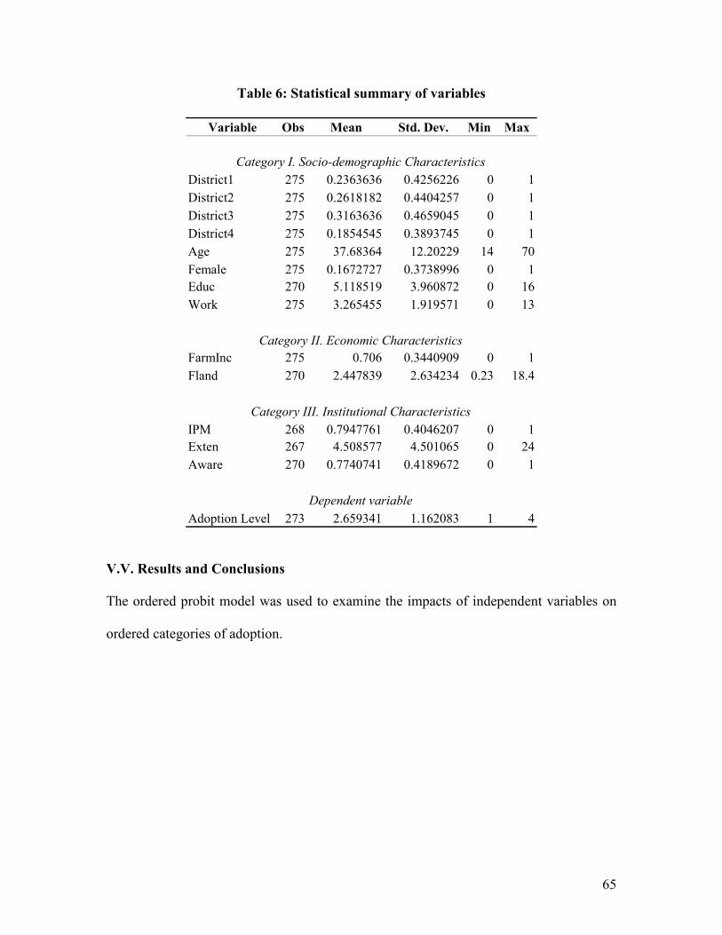
65
Table 6: Statistical summary of variables
Variable Obs Mean Std. Dev. Min Max
District1 275 0.2363636 0.4256226 0 1
District2 275 0.2618182 0.4404257 0 1
District3 275 0.3163636 0.4659045 0 1
District4 275 0.1854545 0.3893745 0 1
Age 275 37.68364 12.20229 14 70
Female 275 0.1672727 0.3738996 0 1
Educ 270 5.118519 3.960872 0 16
Work 275 3.265455 1.919571 0 13
FarmInc 275 0.706 0.3440909 0 1
Fland 270 2.447839 2.634234 0.23 18.4
IPM 268 0.7947761 0.4046207 0 1
Exten 267 4.508577 4.501065 0 24
Aware 270 0.7740741 0.4189672 0 1
Adoption Level 273 2.659341 1.162083 1 4
Dependent variable
Category I. Socio-demographic Characteristics
Category II. Economic Characteristics
Category III. Institutional Characteristics
V.V. Results and Conclusions
The ordered probit model was used to examine the impacts of independent variables on
ordered categories of adoption.

66
Table 7: Summary of the models’ results
Variables
Coeffcient Sig. Coeffcient Sig.
District2 0.82934 0.001***
District3 0.39245 0.089**
District4 0.36498 0.558
Age 0.00014 0.982 0.00161 0.793
Female 1.05229 0.079*0.75417 0.008***
Educ 0.04786 0.015**0.03791 0.050**
Work 0.05739 0.139 0.02864 0.443
FarmInc 0.40345 0.176 0.22352 0.424
Fland -0.00940 0.766 -0.00757 0.801
Exten -0.01228 0.617 -0.03921 0.021**
IPM 0.53253 0.013**0.62835 0.003***
Aware 0.90055 0.000***0.85382 0.000***
n = 248 n = 248
Pseudo R2= 0.1438 Pseudo R
2= 0.1255
* Indicates significance at the 10% level
* * Indicates significance at the 5% level
* * * Indicates significance at the 1% level
Model 1 Model 2
Table 7 summarizes two different models. The sign of the coefficient in the coefficient
columns shows the type of impact, positive or negative, by the particular variable.
According to Borooah (2002, pp.24) the impact on intermediate outcomes can not be
inferred, which means that is it impossible to say whether the probability of no adoption
is higher or lower than low level of adoption, or if the probability of medium adoption is
lower or higher than the probability of high level of IPM adoption.

67
Model 1 includes the full set of variables from which District2, and Aware were
statistically significant at the 1% significance level, while District3, Educ, and IPM was
significant at 5% and Female was statistically significant at 10%. The variable District1
was dropped to avoid the “dummy variable trap.” The variable District2 had a positive
sign, which implied that farmers in District2 had higher probability to be high IPM
adopters and lower probability of no or low IPM adoption then farmers from District1,
ceteris paribus. The implication of District2 was that if all other characteristics were
similar except the district than District2 farmers were more likely to be high IPM
adopters. The implication was not that all Distric2 farmers were higher IPM adopters then
farmers from all the other districts. The sign of the Dirtrict3 variable is the same as
District2 therefore the implication is the same. The variable Female, implies that female
farmers have a higher probability of being high adopters and a lower probability of being
low adopters, compared to male farmers, ceteris paribus. The variable Educ, implies who
have higher education have a higher probability of being high adopters and a lower
probability of being low adopters, compared to farmers that have lower level of
education, ceteris paribus. The variable IPM implies that farmers who have had IPM
training have a higher probability of being high adopters and a lower probability of being
low adopters compared to farmers that haven’t had IPM training, ceteris paribus. The
variable Aware, implies that farmers who are aware of pesticide alternatives have a
higher probability of being high adopters and a lower probability of being low adopters,
than farmers who are aware, ceteris paribus.
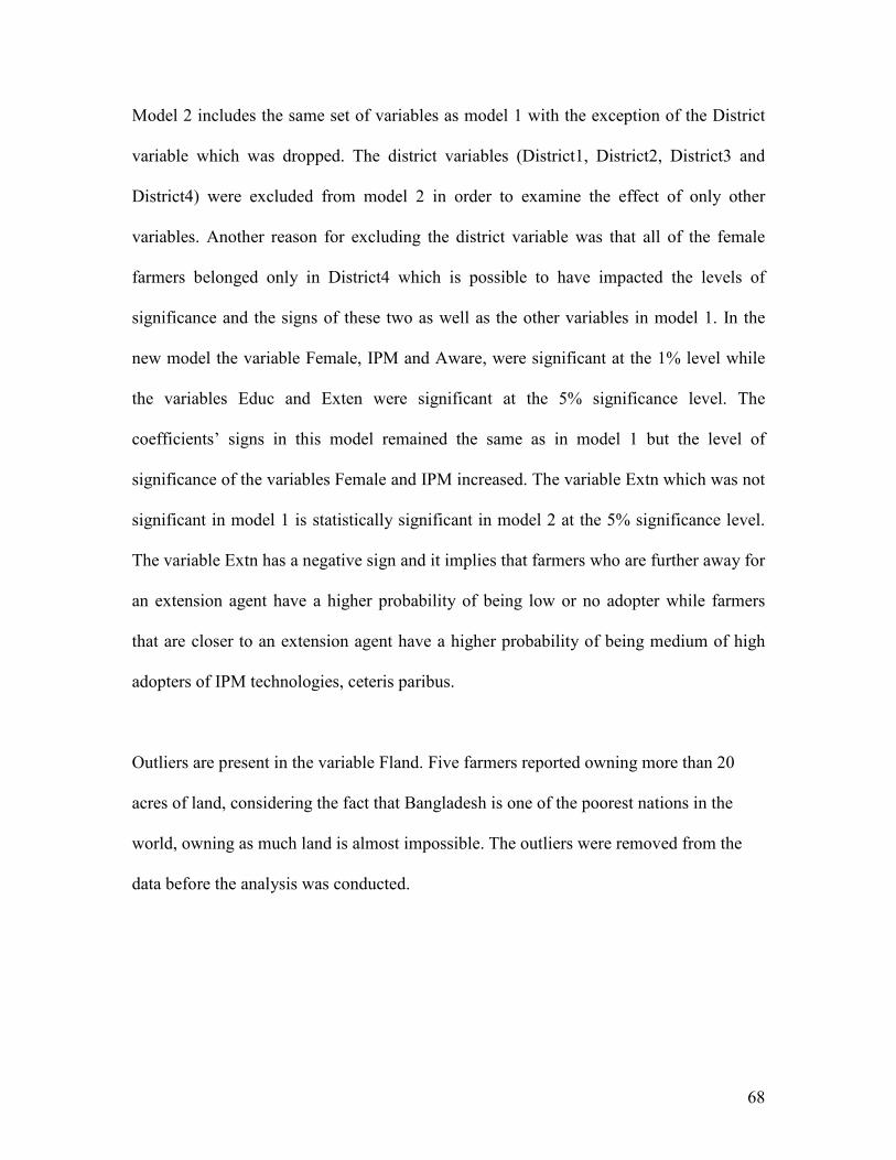
68
Model 2 includes the same set of variables as model 1 with the exception of the District
variable which was dropped. The district variables (District1, District2, District3 and
District4) were excluded from model 2 in order to examine the effect of only other
variables. Another reason for excluding the district variable was that all of the female
farmers belonged only in District4 which is possible to have impacted the levels of
significance and the signs of these two as well as the other variables in model 1. In the
new model the variable Female, IPM and Aware, were significant at the 1% level while
the variables Educ and Exten were significant at the 5% significance level. The
coefficients’ signs in this model remained the same as in model 1 but the level of
significance of the variables Female and IPM increased. The variable Extn which was not
significant in model 1 is statistically significant in model 2 at the 5% significance level.
The variable Extn has a negative sign and it implies that farmers who are further away for
an extension agent have a higher probability of being low or no adopter while farmers
that are closer to an extension agent have a higher probability of being medium of high
adopters of IPM technologies, ceteris paribus.
Outliers are present in the variable Fland. Five farmers reported owning more than 20
acres of land, considering the fact that Bangladesh is one of the poorest nations in the
world, owning as much land is almost impossible. The outliers were removed from the
data before the analysis was conducted.

69
VI. Conclusion and Limitations
There are three different sections in this thesis. The first section is the literature review,
the second section is the economic surplus analysis (Albania, Ecuador, Uganda) and the
third section is the adoption analysis (Bangladesh). Consequently, the conclusions are be
grouped in three categories.
Based on the results from past IPM CRSP impact studies reviewed in the literature
review section it can be concluded that the IPM CRSP technologies have resulted in
positive economic impacts. Previous studies provided information on poverty reduction
for a peanut IPM program in Uganda, nutritional benefits of grafting eggplant for
bacterial wilt in the Philippines, and the environmental benefits of onion IPM in the
Philippines. Please refer to Table 1, for summary of benefits from previous IPM CRSP
impact studies.
The conclusion from the economic surplus analysis (Albania, Ecuador and Uganda) is
that IPM technologies have resulted in positive NPV and positive returns to investment in
all three cases. These findings are similar to the findings of past IPM CRSP impact
studies.
Under the base scenario the NPV of the tomato IPM Program in Albania was
approximately USD $8 million. Increasing the rate of adoption increased the NPV to
about USD $22 million6 for the 15 year period. In the second sensitivity analysis, the
6 Refer to Appendix C for the sensitivity analysis table

70
percent change in cost per hectare rose to 25% which resulted in a decrease of the NVP to
about USD $5 million over the 15 year period, at a 5% discount rate.
Under the baseline scenario for the Plantain IPM Program in Ecuador, the NPV was
found to be approximately USD $7 million over 15 years at a 5% discount rate. The IRR
was 110%. Reducing the yield change to 70% resulted in a lower NPV of benefits of
approximately USD $4 million and an IRR’s of 89%.
Under the base scenario for the Tomato IPM Program in Uganda, it was found that the
NPV of benefits from adopting the IPM practices using a 5% discount rate was about
USD $1 million, and the IRR was 169%. Increasing the adoption rate to 70% yielded a
NPV of about $ 2.5 million and IRR of 174%. Changing the percent change in cost per
hectare to 25% decreased the NPV to about USD $0.58 million (5% discount rate) and
the IRR to 133% when the maximum adoption of 25% was achieved. Based on the
different combination of practices Case1 and Case2 scenarios were conducted. The Case1
scenario yielded NPV of approximately $0.03 million and IRR was 43% when adoption
reaches a maximum of 25%. The Case2 scenario resulted in a new NPV of approximately
$0.8 million (at 5% discount rate) and IRR of 270% when the adoption rate was 25%.
The analysis on adoption of IPM technologies in Bangladesh is the last section. The
conclusion from this section is that the institutional factors are particularly important and
significant for the adoption of IPM technologies. In this study the impact of the variables
in both models was found to be consistent, while some studies had found opposing
indeterminate impacts due to changes in the coefficients sign throughout the different

71
models. As expected the level of education, being a female farmer, IPM training and the
awareness of pesticide alternatives were found to be significant factors positively
affecting the adoption of IPM technologies. The age variable was expected to have a
negative impact on the level of IPM adoption, but the models demonstrated that age had a
positive impact. The impact of the age variable was not statistically significant.
VI.I. Implications for further research
Some of the IPM CRSP impact studies were conducted in languages other than English.
Even though this thesis attempted to include most of the available IPM CRSP impact
studies, there still are and will be other studies that have not been included. Some studies
are currently in progress, while others are conducted in remote areas of the world and are
not published etc.
With regard to the economic surplus analysis, one implication for further research is to
include one example from all the site areas. This thesis included three different examples
from three different sites. If all IPM CRSP sites had responded to the scientist-
questionnaire, the results would have provided a better picture of the current situation in
the different parts of the world.
Adoption analyses provide useful and necessary information that helps in the process of
IPM technology dissemination. The adoption analysis of IPM technologies in Bangladesh
was based on a survey conducted for assessing the adoption of pheromones for cucurbit
crops. More accurate results could be obtained if the survey was conducted specifically

72
for assessing the adoption factors for IPM technologies. The results would also be more
accurate if the whole country (Bangladesh) was surveyed. However, surveying the whole
country is time consuming and costly and therefore only the major vegetable areas were
surveyed.
The IPM CRSP has been helpful and beneficial to farmers around the world. Further up-
to-date research is necessary to measure the impacts of the IPM CRSP.

73
References:
Adesina, A.A., D. Mbila, G.B. Nkamleu, and D. Endamana. 2000. "Econometric analysis
of the determinants of adoption of alley farming by farmers in the forest zone of southwest Cameroon." Agriculture, Ecosystems & Environment 80(3): 255-265.
Alwang J.A., Weller S.C., Sanchez G.E., Calderon L., Edwards C.R., Hamilton S., Williams R., Ellis M., Suarez C., Barrera V., Crissman C., Norton G W. 2005. “Developing IPM Packages in Latin America.” In G.W. Norton, E.A. Heinrichs, G.C. Luther, and M.E. Irwin eds. Globalizing integrated pest management: A
participatory research process. Ames IA: Blackwell Publishing. pp. 71-94. Antle, J.M. and S.M. Capalbo. 1995. Measurement and Evaluation of the Impacts of
Agricultural Chemical Use: A Framework for Analysis. In Impact of Pesticides on
Farmer Health and the Rice Environment. P.L. Pingali and P.A. Roger, eds. Norwell, MA, Kluwer Academic Publishers, 1995.
Alponi, A.J. “Adoption of IPM technology in Vegetables and its relative advantages over farmers practices in some selected areas of Bangladesh.” MS thesis. Bangladesh Agricultural University. 2003
Alston, J.M., G.W.Norton., and P.G. Pardey. 1998. Science under Scarcity, CAB International
Baez, C. “Potential Economic Benefits from Plantain Integrated Pest Management Adoption: The Case of Coastal Rural Households in Ecuador.” Ms thesis, Virginia Polytechnic Institute and State University. 2004
Borooah, V. K. 2002. Logit and probit: Ordered and multinomial models. Thousand Oaks, CA: Sage Publications.
Brown, M.L. 1979. Farm Budgets: From Farm Income Analysis to Agricultural Project
Analysis, World Bank staff occasional papers, no. 29. Baltimore: Published for the World Bank [by] the Johns Hopkins University Press.
Chaves, B., and J. Riley. 2001 "Determination of factors influencing integrated pest management adoption in coffee berry borer in Colombian farms." Agriculture,
Ecosystems & Environment 87,(2): 159-177. Cole, D.C., S. Sherwood, C. Crissman, V. Barrera, and P. Espinosa. 2002. "Pesticides
and Health in Highland Ecuadorian Potato Production: Assessing Impacts and Developing Responses." International Journal of Occupational and
Environmental Health 8(3): 182-190. Cuyno, L.C.M. 1999. “An economic evaluation of the health and environmental benefits
of the IPM program (IPM CRSP) in the Philippines.” PhD dissertation, Virginia Polytechnic Institute and State University.
Daku, L.S. 2002. “Assessing Farm-level and Aggregate Economic Impacts of Olive Integrated Pest Management Programs in Albania: An Ex-Ante Analysis.” PhD dissertation, Virginia Polytechnic Institute and State University.
Debass, T. 2000. “Economic Impact Assessment of IPM CRSP Activities in Bangladesh and Uganda: A GIS Application.” MS thesis, Virginia Polytechnic Institute and State University.
De Souza-Filho, H. M., T. Young, and M. P. Burton. 1999. “Factors Influencing the Adoption of Sustainable Agricultural Technologies Evidence from the State of
74
Espírito Santo, Brazil.” Technological Forecasting and Social Change 60: 97-112.
EPA, Environmental Protection Agency. (2007). What is IPM. Retrieved 02/25/08, from http://www.epa.gov/pesticides/ipm/brochure/whatipm.htm
Erbaugh J.M., J.Caldwell, S. Kyamanywa, K.T. Gamby, and K. Moore. 2005. “Developing IPM Packages in Africa.” In G.W. Norton, E.A. Heinrichs, G.C. Luther, and M.E. Irwin eds. Globalizing integrated pest management: A
participatory research process. Ames IA: Blackwell Publishing. pp. 51-69. FAOSTAT. (2008) Food and Agricultural Organization Statistical Data Base: FAOSTAT
Albania: Tomatoes.” Retrieved 09/15/08 from http://faostat.fao.org/site/567/DesktopDefault.aspx?PageID=567#ancor
__________.(2008a). Food and Agricultural Organization Statistical Data Base: FAOSTAT Ecuador: Plantains. Retrieved 08/04/08, from
http://faostat.fao.org/site/567/DesktopDefault.aspx?PageID=567. __________. (2008b). Food and Agricultural Organization Statistical Data Base:
FAOSTAT Uganda: Tomatoes.” Retrieved 09/20/08 from http://faostat.fao.org/site/567/DesktopDefault.aspx?PageID=567#ancor
FAO. (2008). Major Food and Agricultural Commodities and Producers: Albania. Retrieved 18/15/08, from http://www.fao.org/es/ess/top/country.html?lang=en&country=3
Feder G., R.E. Just, and D. Zilberman. 1985. "Adoption of Agricultural Innovations in Developing Countries: A Survey." Economic Development and Cultural Change 33(2): 255-298.
Feder G., and R. Slade. 1984. "The Acquisition of Information and the Adoption of New Technology." Amer. J. of Agri. Econ. 66(3): 312-320.
Feder, G. and D. L. Umali. 1993. ”The Adoption of Agricultural Innovations A Review.” Technological Forecasting and Social Change 43: 215-239.
IPM CRSP. (2008). IPM CRSP Countries at a Glance. Retrieved 09/08/08, from http://www.oired.vt.edu/ipmcrsp/IPM_2008/Countries.htm.
__________. (2008a). What do we do. Retrieved 02/23/2008, from http://www.oired.vt.edu/ipmcrsp/IPM_2008/What_We_Do/what_is_ipm.htm
__________. (2008b). IPM CRSP IPM Goals and Objectives. Retrieved 09/08/08, from http://www.oired.vt.edu/ipmcrsp/IPM_2008/What_We_Do/goals.htm
__________. (2008c). "What do we do: Gender and IPM." Retrieved 02/23/2008, from: http://www.oired.vt.edu/ipmcrsp/IPM_2008/What_We_Do/gender.htm
Katsoyannos, P. 1992. Olive Pests and Their Control in the Near East. United Nations, Food and Agriculture Organization: Plant Production and Protection Paper No. 115. Rome.
Lawrence J., S. Tolin, C. Edwards, S. Fleischer, D.M. Jackson, D. Clarke-Harris, S. McDonald, K. Dalip, and P. Chung. 2005. “Developing IPM Packages in the Caribbean.” In G.W. Norton, E.A. Heinrichs, G.C. Luther, and M.E. Irwin eds.
Globalizing integrated pest management: A participatory research process. Ames IA: Blackwell Publishing. pp. 95-119.
Mamaril, C.B. and G.W. Norton. 2006. "Economic evaluation of transgenic pest resistant rice in the Philippines and Vietnam." Quarterly Journal of International
Agriculture 45(2): 127-144.

75
Matonan Z., and Abacus. (2009). Country Report Albania. Retrieved on April 30, 2009 from: http://www.povrce.com/index.cgi?P=gen&A=FAO&HTM=10091
McDonald, S.A., B. Nault, and S.A. Tolin 2004. “Efficacy of Stylet-Oil® in suppressing the spread of TEV infections in a ‘Scotch Bonnet’ pepper (Capsicum chinense Jacquin) in field in Jamaica.” Tropical Agriculture 81(1): 54-60.
Miller S.A., Karim A.M.N.R., Baltazar A.M., Rajotte., Norton G.W. 2005. “Developing IPM Packages in Asia.” In G.W. Norton, E.A. Heinrichs, G.C. Luther, and M.E. Irwin eds. Globalizing integrated pest management: A participatory research
process. Ames IA: Blackwell Publishing. pp. 27-50. Mishra, S. 2003. “An Ex-Ante Economic Impact Assessment of Bt Eggplant in
Bangladesh, the Philippines and India.” MS thesis, Virginia Polytechnic Institute and State University.
Moyo, S., G.W. Norton, J. Alwang, I. Rhinehart, and C.M. Deom. 2007. “Peanut Research and Poverty Reduction: Impacts of Variety Improvement to Control Peanut Viruses in Uganda.” Amer. J. Agri. Econ. 89: 448-460.
Mullen, J.D., G.W. Norton, and D.W. Reaves. 1997. "Economic Analysis of Environmental Benefits of Integrated Pest Management." Journal of Agricultural
and Applied Economics 29(2): 243-253. Mutuc, M.M.E. 2003. “Increase in Calorie Intake Due to Eggplant Grafting: Proof of
Concept With the Use of Minimum Datasets.” MS thesis, Virginia Polytechnic Institute and State University.
Nouhoheflin T, O. Coulibaly, S. Soumare, and G.W. Norton. 2009. “Tomato Baseline Survey and Impact Assessment of Research to Reduce Tomato Viruses in Mali.” Unpublished Manuscript, Department of Agricultural and Applied Economics, Virginia Tech
Norton G.W., K. Moore, D. Quishpe, V. Barrera, T. Debass, S. Moyo, and D.B. Taylor. 2005. “Evaluating Socio-Economic Impacts of IPM.” In G.W. Norton, E.A. Heinrichs, G.C. Luther, and M.E. Irwin eds. Globalizing integrated pest
management: A participatory research process. Ames IA: Blackwell Publishing. pp. 241.
Norton, G.W., and J. Mullen. 1994. “Economic Evaluation of Integrated Pest Management Programs: A Literature Review.” MS thesis, Virginia Polytechnic Institute and State University.
Pfeifer D., J. Tedeschini, L. Daku, M. Hasani, R. Uka, B. Stamo, and B. Ferraj. 2005. “Developing IPM Packages in Eastern Europe: Participatory IPM Research in Albanian Olives.” In G.W. Norton, E.A. Heinrichs, G.C. Luther, and M.E. Irwin eds. Globalizing integrated pest management: A participatory research process.
Ames IA: Blackwell Publishing. pp. 27-50. Project SICA/MAC. (2002). III Censo Nacional Agropecuario. Retrieved from
http://www.sica.gov.ec/censo/index.htm Rakshit, A. 2008. “Integrated Pest Management in Bangladesh: An Impact Assessment of
Pheromone Adoption for Cucurbit Crops.” MS thesis, Virginia Polytechnic Institute and State University.

76
Rauniyar, G. P., and F. M. Goode. 1996. "Managing Green Revolution Technology: An Analysis of a Differential Practice Combination in Swaziland." Economic
Development and Cultural Change 44(2): 413-437. Rickard. B.J., and D. A. Sumner. “EU Support Reductions Would Benefit California
Tomato Growers and Processors.” California Agriculture. 60 (Oct.-Dec. 2006): 207-210
Steinemann, A.C., W.C. Apgar, H.J. Brown. 2005. Microeconomics for Public Decisions, Thomson South-Western. USAID. (2007). "Agriculture." Retrieved 02/23/08, from
http://www.usaid.gov/our_work/agriculture/ USAID. (2009). “USAID Mission in Bangladesh: Education.” Retrieved 02/06/09 from
http://www.usaid.gov/bd/programs/education.html US Department of State. 2008. Background 7ote: Bangladesh. Retrieved 11/18/08, from
http://www.state.gov/r/pa/ei/bgn/3452.htm Victoria, M.V. 2007. "Agricultural Technology in Bangladesh: A Study on non-farm
Labor and adoption by Gender." MS thesis, Virginia Polytechnic Institute and State University.
World Bank. (2008). Bangladesh: Data and Statistics - Poverty at a Glance. Retrieved 11/18/08, from http://devdata.worldbank.org/AAG/bgd_aag.pdf.
Weller, S.C., G.E. Sanchez, C.R. Edwards, and G.H. Sullivan. 2002. “IPM CRSP success in NTAE crops leads to sustainable trade for developing countries.” Sustainable
Development International 5: 135 - 138 Wooldridge, J. M. 2002. Econometric analysis of cross section and panel data.
Cambridge, Mass: MIT Press. Wooldridge, J. M. 2006. Introductory econometrics: A modern approach. Mason, OH:
Thomson/South-Western.

77
Appendix A: A sample scientist-questionnaire.
Scientist Questionnaire (Albania)
Commodity: Tomato
Respondent(s)
Name(s): _________________________ Date: __________________________
Specialty: ______________________
Years of experience on tomato: _______ Please describe the IPM practice(s) on tomato: ________________________________________________________________________________________________________________________________________________________________________________________________________________________ 1. What is the percent yield change (if any) per hectare (compared to previous practice) for farmers who adopt the tomato IPM practice(s) developed by the IPM CRSP_______% 2. What is your estimate of the percent change in cost per hectare (if any) for each of the
following production inputs for farmers who adopt the tomato IPM practices?
Most Likely Cost Change
Input Share of
total costs
Decrease No Change Increase Percent
Change
Labor
Pesticides
Seeds and fertilizer
Other
3. If pesticide use was reduced, which pesticides?_______________________________
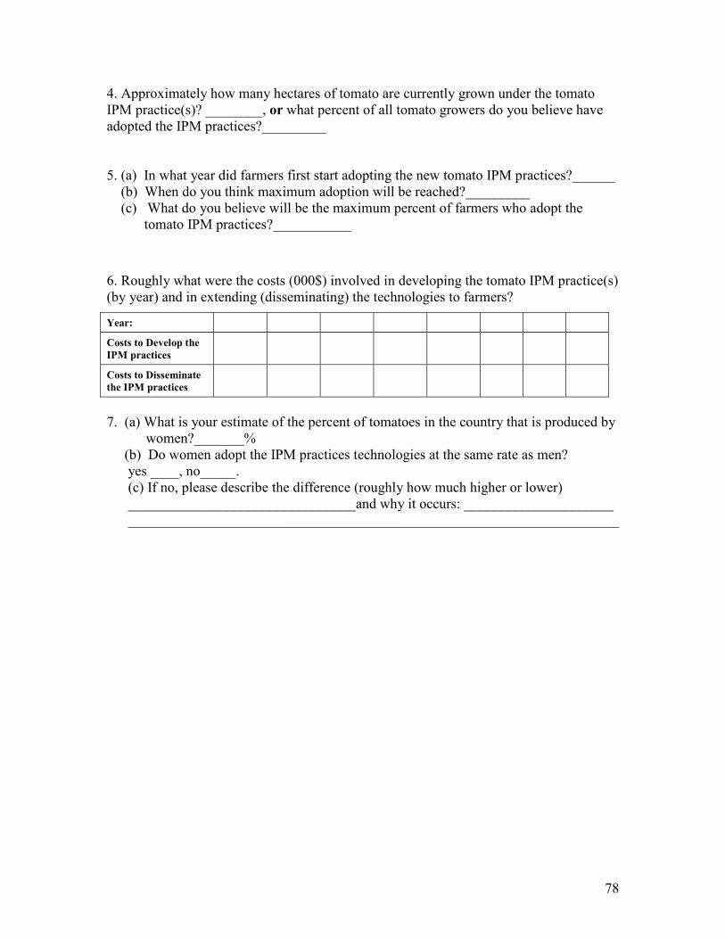
78
4. Approximately how many hectares of tomato are currently grown under the tomato IPM practice(s)? ________, or what percent of all tomato growers do you believe have adopted the IPM practices?_________ 5. (a) In what year did farmers first start adopting the new tomato IPM practices?______ (b) When do you think maximum adoption will be reached?_________ (c) What do you believe will be the maximum percent of farmers who adopt the
tomato IPM practices?___________
6. Roughly what were the costs (000$) involved in developing the tomato IPM practice(s) (by year) and in extending (disseminating) the technologies to farmers?
Year:
Costs to Develop the
IPM practices
Costs to Disseminate
the IPM practices
7. (a) What is your estimate of the percent of tomatoes in the country that is produced by women?_______% (b) Do women adopt the IPM practices technologies at the same rate as men?
yes ____, no_____. (c) If no, please describe the difference (roughly how much higher or lower) ________________________________and why it occurs: _____________________ _____________________________________________________________________
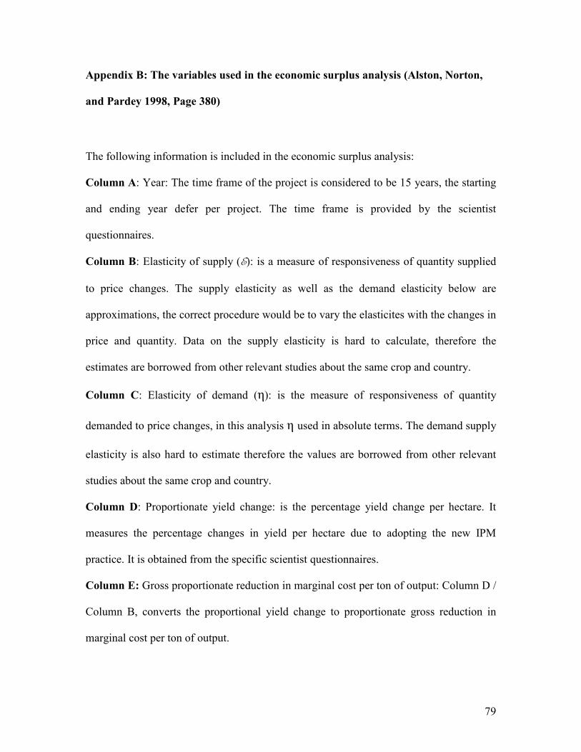
79
Appendix B: The variables used in the economic surplus analysis (Alston, 6orton,
and Pardey 1998, Page 380)
The following information is included in the economic surplus analysis:
Column A: Year: The time frame of the project is considered to be 15 years, the starting
and ending year defer per project. The time frame is provided by the scientist
questionnaires.
Column B: Elasticity of supply (E): is a measure of responsiveness of quantity supplied
to price changes. The supply elasticity as well as the demand elasticity below are
approximations, the correct procedure would be to vary the elasticites with the changes in
price and quantity. Data on the supply elasticity is hard to calculate, therefore the
estimates are borrowed from other relevant studies about the same crop and country.
Column C: Elasticity of demand (η): is the measure of responsiveness of quantity
demanded to price changes, in this analysis η used in absolute terms. The demand supply
elasticity is also hard to estimate therefore the values are borrowed from other relevant
studies about the same crop and country.
Column D: Proportionate yield change: is the percentage yield change per hectare. It
measures the percentage changes in yield per hectare due to adopting the new IPM
practice. It is obtained from the specific scientist questionnaires.
Column E: Gross proportionate reduction in marginal cost per ton of output: Column D /
Column B, converts the proportional yield change to proportionate gross reduction in
marginal cost per ton of output.

80
Column F: Proportionate change in variable input cost per hectare, if any, to achieve the
expected yield change.
Column G: Proportionate change in variable input cost per ton: Column F / (1 + Column
D), the proportionate input cost change per hectare is converted to the proportionate input
cost change per ton.
Column H: Net change: Column E – Column G, provides the net effects of the variable
input changes associated with the yield change resulting in the maximum potential net
change in marginal cost per ton of output.
Column I: Probability of success: measures the probability that the research will achieve
the yield change in column D.
Column J: Adoption rate: Provides the adoption rate relative to the years from the
commencement of research.
Column K: Proportionate supply shift per year of the K shift: Column H * Column I *
Column J, gives the proportionate shift down of the supply curve.
Column L: Proportionate reduction in price or Z shift relative to it’s initial value, due to
the supply shift: in the case of closed economy the Z shift is obtained (Column B *
Column K) / (Column B + Column C). In the large open economy case Z is obtained
(Column B * Column K) / (Column B + sA * Column C + ( 1 - sA)*ηB
E
). Note sA and ηB
E
are defined in chapter III.
Column M: Price: is the average price, the time over which prices are averaged differs
for each economic surplus analysis depending on the time frame and the data available
from FAO STAT.
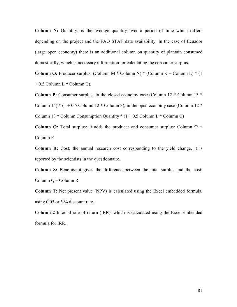
81
Column 6: Quantity: is the average quantity over a period of time which differs
depending on the project and the FAO STAT data availability. In the case of Ecuador
(large open economy) there is an additional column on quantity of plantain consumed
domestically, which is necessary information for calculating the consumer surplus.
Column O: Producer surplus: (Column M * Column N) * (Column K – Column L) * (1
+ 0.5 Column L * Column C).
Column P: Consumer surplus: In the closed economy case (Column 12 * Column 13 *
Column 14) * (1 + 0.5 Column 12 * Column 3), in the open economy case (Column 12 *
Column 13 * Column Consumption Quantity * (1 + 0.5 Column L * Column C)
Column Q: Total surplus: It adds the producer and consumer surplus: Column O +
Column P
Column R: Cost: the annual research cost corresponding to the yield change, it is
reported by the scientists in the questionnaire.
Column S: Benefits: it gives the difference between the total surplus and the cost:
Column Q – Column R.
Column T: Net present value (NPV) is calculated using the Excel embedded formula,
using 0.05 or 5 % discount rate.
Column 2 Internal rate of return (IRR): which is calculated using the Excel embedded
formula for IRR.
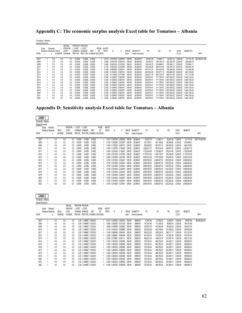
82
Appendix C: The economic surplus analysis Excel table for Tomatoes – Albania
Tomatoes - AlbaniaClosed Economy
GROSS PROPOR. PROPOR.Suply Demand PROPOR. I. COST I. COST PROB ADOPTElasticity Elasticity YIELD COST CHANGE CHANGE NET OF RATE K Z PRICE QUANTITY PS CS TS COST BENEFITS
YEAR E ƞ CHANGE CHANGE PER HA. PER TON CHANGESUCCESS $/ton metric tons/year $ U.S NPV
2007 1 0.5 0.5 0.5 -0.0039 -0.0026 0.5026 1 0.015 0.007539 0.005026 308.59 26,969.87 20,941.05 41,882.11 62,823.16 1,650.00 61,173.16 $8,358,811.982008 1 0.5 0.5 0.5 -0.0039 -0.0026 0.5026 1 0.060 0.030156 0.020104 308.59 26,969.87 84,079.57 168,159.13 252,238.70 2,300.00 249,938.702009 1 0.5 0.5 0.5 -0.0039 -0.0026 0.5026 1 0.090 0.045234 0.030156 308.59 26,969.87 126,434.70 252,869.41 379,304.11 2,500.00 376,804.112010 1 0.5 0.5 0.5 -0.0039 -0.0026 0.5026 1 0.130 0.065338 0.043559 308.59 26,969.87 183,235.25 366,470.50 549,705.76 2,800.00 546,905.762011 1 0.5 0.5 0.5 -0.0039 -0.0026 0.5026 1 0.180 0.090468 0.060312 308.59 26,969.87 254,761.53 509,523.05 764,284.58 3,000.00 761,284.582012 1 0.5 0.5 0.5 -0.0039 -0.0026 0.5026 1 0.200 0.100520 0.067013 308.59 26,969.87 283,535.55 567,071.10 850,606.65 3,500.00 847,106.652013 1 0.5 0.5 0.5 -0.0039 -0.0026 0.5026 1 0.230 0.115598 0.077065 308.59 26,969.87 326,871.79 653,743.57 980,615.36 3,500.00 977,115.362014 1 0.5 0.5 0.5 -0.0039 -0.0026 0.5026 1 0.250 0.125650 0.083767 308.59 26,969.87 355,879.41 711,758.81 1,067,638.22 3,500.00 1,064,138.222015 1 0.5 0.5 0.5 -0.0039 -0.0026 0.5026 1 0.250 0.125650 0.083767 308.59 26,969.87 355,879.41 711,758.81 1,067,638.22 3,500.00 1,064,138.222016 1 0.5 0.5 0.5 -0.0039 -0.0026 0.5026 1 0.250 0.125650 0.083767 308.59 26,969.87 355,879.41 711,758.81 1,067,638.22 3,500.00 1,064,138.222017 1 0.5 0.5 0.5 -0.0039 -0.0026 0.5026 1 0.250 0.125650 0.083767 308.59 26,969.87 355,879.41 711,758.81 1,067,638.22 3,500.00 1,064,138.222018 1 0.5 0.5 0.5 -0.0039 -0.0026 0.5026 1 0.250 0.125650 0.083767 308.59 26,969.87 355,879.41 711,758.81 1,067,638.22 3,500.00 1,064,138.222019 1 0.5 0.5 0.5 -0.0039 -0.0026 0.5026 1 0.250 0.125650 0.083767 308.59 26,969.87 355,879.41 711,758.81 1,067,638.22 3,500.00 1,064,138.222020 1 0.5 0.5 0.5 -0.0039 -0.0026 0.5026 1 0.250 0.125650 0.083767 308.59 26,969.87 355,879.41 711,758.81 1,067,638.22 3,500.00 1,064,138.222021 1 0.5 0.5 0.5 -0.0039 -0.0026 0.5026 1 0.250 0.125650 0.083767 308.59 26,969.87 355,879.41 711,758.81 1,067,638.22 3,500.00 1,064,138.222022 1 0.5 0.5 0.5 -0.0039 -0.0026 0.5026 1 0.250 0.125650 0.083767 308.59 26,969.87 355,879.41 711,758.81 1,067,638.22 3,500.00 1,064,138.22
Appendix D: Sensitivity analysis Excel table for Tomatoes – Albania
Tomatoes - AlbaniaClosed Economy
Suply Demand PROPOR. I. COST I. COST PROB ADOPTElasticity Elasticity YIELD COST CHANGE CHANGE NET OF RATE K Z PRICE QUANTITY TS CS PS COST BENEFIT
YEAR ɛ ƞ CHANGE CHANGE PER HA. PER TON CHANGE SUCCESS $/ton metric tons/year $ U.S NPV
_______________________________________________________________________________________________________________________________________________________________________________________________________________________________________________ ________________ ________________________________
2007 1 0.5 0.5 0.5 -0.0039 -0.0026 0.5026 1 0.015 0.007539 0.005026 308.59 26,969.87 62,823.16 41,882.11 20,941.05 1,650.00 61,173.16 $22,714,675.682008 1 0.5 0.5 0.5 -0.0039 -0.0026 0.5026 1 0.100 0.050260 0.033507 308.59 26,969.87 421,799.41 281,199.60 140,599.80 2,300.00 419,499.412009 1 0.5 0.5 0.5 -0.0039 -0.0026 0.5026 1 0.200 0.100520 0.067013 308.59 26,969.87 850,606.65 567,071.10 283,535.55 2,500.00 848,106.652010 1 0.5 0.5 0.5 -0.0039 -0.0026 0.5026 1 0.300 0.150780 0.100520 308.59 26,969.87 1,286,421.75 857,614.50 428,807.25 2,800.00 1,283,621.752011 1 0.5 0.5 0.5 -0.0039 -0.0026 0.5026 1 0.400 0.201040 0.134027 308.59 26,969.87 1,729,244.68 1,152,829.79 576,414.89 3,000.00 1,726,244.682012 1 0.5 0.5 0.5 -0.0039 -0.0026 0.5026 1 0.500 0.251300 0.167533 308.59 26,969.87 2,179,075.46 1,452,716.97 726,358.49 3,500.00 2,175,575.462013 1 0.5 0.5 0.5 -0.0039 -0.0026 0.5026 1 0.600 0.301560 0.201040 308.59 26,969.87 2,635,914.09 1,757,276.06 878,638.03 3,500.00 2,632,414.092014 1 0.5 0.5 0.5 -0.0039 -0.0026 0.5026 1 0.700 0.351820 0.234547 308.59 26,969.87 3,099,760.55 2,066,507.03 1,033,253.52 3,500.00 3,096,260.552015 1 0.5 0.5 0.5 -0.0039 -0.0026 0.5026 1 0.700 0.351820 0.234547 308.59 26,969.87 3,099,760.55 2,066,507.03 1,033,253.52 3,500.00 3,096,260.552016 1 0.5 0.5 0.5 -0.0039 -0.0026 0.5026 1 0.700 0.351820 0.234547 308.59 26,969.87 3,099,760.55 2,066,507.03 1,033,253.52 3,500.00 3,096,260.552017 1 0.5 0.5 0.5 -0.0039 -0.0026 0.5026 1 0.700 0.351820 0.234547 308.59 26,969.87 3,099,760.55 2,066,507.03 1,033,253.52 3,500.00 3,096,260.552018 1 0.5 0.5 0.5 -0.0039 -0.0026 0.5026 1 0.700 0.351820 0.234547 308.59 26,969.87 3,099,760.55 2,066,507.03 1,033,253.52 3,500.00 3,096,260.552019 1 0.5 0.5 0.5 -0.0039 -0.0026 0.5026 1 0.700 0.351820 0.234547 308.59 26,969.87 3,099,760.55 2,066,507.03 1,033,253.52 3,500.00 3,096,260.552020 1 0.5 0.5 0.5 -0.0039 -0.0026 0.5026 1 0.700 0.351820 0.234547 308.59 26,969.87 3,099,760.55 2,066,507.03 1,033,253.52 3,500.00 3,096,260.552021 1 0.5 0.5 0.5 -0.0039 -0.0026 0.5026 1 0.700 0.351820 0.234547 308.59 26,969.87 3,099,760.55 2,066,507.03 1,033,253.52 3,500.00 3,096,260.552022 1 0.5 0.5 0.5 -0.0039 -0.0026 0.5026 1 0.700 0.351820 0.234547 308.59 26,969.87 3,099,760.55 2,066,507.03 1,033,253.52 3,500.00 3,096,260.55
Tomatoes - AlbaniaClosed Economy _____________________________________________________________________________________________________________
GROSS PROPOR. PROPOR.Suply Demand PROPOR. I. COST I. COST PROB ADOPTElasticity Elasticity YIELD COST CHANGE CHANGE NET OF RATE K Z PRICE QUANTITY TS CS PS COST BENEFIT
YEAR ɛ ƞ CHANGE CHANGE PER HA. PER TON CHANGE SUCCESS $/ton metric tons/year $ U.S NPV
2007 1 0.5 0.5 0.5 0.25 0.166667 0.333333 1 0.015 0.005000 0.003333 308.59 26969.87 41,647.84 27,765.23 13,882.61 1,650.00 39,997.84 $5,498,633.822008 1 0.5 0.5 0.5 0.25 0.166667 0.333333 1 0.060 0.020000 0.013333 308.59 26969.87 167,007.48 111,338.32 55,669.16 2,300.00 164,707.482009 1 0.5 0.5 0.5 0.25 0.166667 0.333333 1 0.090 0.030000 0.020000 308.59 26969.87 250,927.35 167,284.90 83,642.45 2,500.00 248,427.352010 1 0.5 0.5 0.5 0.25 0.166667 0.333333 1 0.130 0.043333 0.028889 308.59 26969.87 363,252.06 242,168.04 121,084.02 2,800.00 360,452.062011 1 0.5 0.5 0.5 0.25 0.166667 0.333333 1 0.180 0.060000 0.040000 308.59 26969.87 504,351.50 336,234.33 168,117.17 3,000.00 501,351.502012 1 0.5 0.5 0.5 0.25 0.166667 0.333333 1 0.200 0.066667 0.044444 308.59 26969.87 561,007.04 374,004.70 187,002.35 3,500.00 557,507.042013 1 0.5 0.5 0.5 0.25 0.166667 0.333333 1 0.230 0.076667 0.051111 308.59 26969.87 646,221.55 430,814.37 215,407.18 3,500.00 642,721.552014 1 0.5 0.5 0.5 0.25 0.166667 0.333333 1 0.250 0.083333 0.055556 308.59 26969.87 703,185.34 468,790.23 234,395.11 3,500.00 699,685.342015 1 0.5 0.5 0.5 0.25 0.166667 0.333333 1 0.250 0.083333 0.055556 308.59 26969.87 703,185.34 468,790.23 234,395.11 3,500.00 699,685.342016 1 0.5 0.5 0.5 0.25 0.166667 0.333333 1 0.250 0.083333 0.055556 308.59 26969.87 703,185.34 468,790.23 234,395.11 3,500.00 699,685.342017 1 0.5 0.5 0.5 0.25 0.166667 0.333333 1 0.250 0.083333 0.055556 308.59 26969.87 703,185.34 468,790.23 234,395.11 3,500.00 699,685.342018 1 0.5 0.5 0.5 0.25 0.166667 0.333333 1 0.250 0.083333 0.055556 308.59 26969.87 703,185.34 468,790.23 234,395.11 3,500.00 699,685.342019 1 0.5 0.5 0.5 0.25 0.166667 0.333333 1 0.250 0.083333 0.055556 308.59 26969.87 703,185.34 468,790.23 234,395.11 3,500.00 699,685.342020 1 0.5 0.5 0.5 0.25 0.166667 0.333333 1 0.250 0.083333 0.055556 308.59 26969.87 703,185.34 468,790.23 234,395.11 3,500.00 699,685.342021 1 0.5 0.5 0.5 0.25 0.166667 0.333333 1 0.250 0.083333 0.055556 308.59 26969.87 703,185.34 468,790.23 234,395.11 3,500.00 699,685.342022 1 0.5 0.5 0.5 0.25 0.166667 0.333333 1 0.250 0.083333 0.055556 308.59 26969.87 703,185.34 468,790.23 234,395.11 3,500.00 699,685.34
CASE 1
CASE 2

83
Appendix E: Economic Surplus analysis Excel table for Plantain – Ecuador
Plantain - Ecuador
GROSS PROPOR. PROPOR.Suply Demand % PROPOR. I. COST I. COST PROBElasticity Elasticity YIELD COST CHANGE CHANGE NET OF ADOPT QUANTITY QUANTITY CS PS TS COST BENEFIT
YEAR EA ƞA CHANGECHANGE PER HA. PER TON CHANGE SUCCESS RATE K Z PRICE Produced Consumed $ U.S NPV IRR
_______________________________________________________________________________________________________________________________________________________________________________________________________________________________________________ ________________________________________________
1999 1 0.3 1 1 0.3688 0.1844 0.8156 1 0 0 0 53.3333 801,379.33 467,722.33 0.00 0.00 0.00 26,000.00 -26,000.00 $6,502,488.75 110%2000 1 0.3 1 1 0.3688 0.1844 0.8156 1 0 0 0 53.3333 801,379.33 467,722.33 0.00 0.00 0.00 23,000.00 -23,000.002001 1 0.3 1 1 0.3688 0.1844 0.8156 1 0 0 0 53.3333 801,379.33 467,722.33 0.00 0.00 0.00 21,000.00 -21,000.002002 1 0.3 1 1 0.3688 0.1844 0.8156 1 0 0 0 53.3333 801,379.33 467,722.33 0.00 0.00 0.00 41,500.00 -41,500.002003 1 0.3 1 1 0.3688 0.1844 0.8156 1 0.01 0.00816 0.00014 53.3333 801,379.33 467,722.33 3,441.44 342,716.65 346,158.08 25,000.00 321,158.082004 1 0.3 1 1 0.3688 0.1844 0.8156 1 0.015 0.01223 0.00021 53.3333 801,379.33 467,722.33 5,162.21 514,092.70 519,254.91 20,000.00 499,254.912005 1 0.3 1 1 0.3688 0.1844 0.8156 1 0.02 0.01631 0.00028 53.3333 801,379.33 467,722.33 6,883.02 685,480.57 692,363.58 14,000.00 678,363.582006 1 0.3 1 1 0.3688 0.1844 0.8156 1 0.022 0.01794 0.0003 53.3333 801,379.33 467,722.33 7,571.35 754,039.02 761,610.38 4,000.00 757,610.382007 1 0.3 1 1 0.3688 0.1844 0.8156 1 0.028 0.02284 0.00039 53.3333 801,379.33 467,722.33 9,636.38 959,725.74 969,362.13 4,000.00 965,362.132008 1 0.3 1 1 0.3688 0.1844 0.8156 1 0.03 0.02447 0.00041 53.3333 801,379.33 467,722.33 10,324.74 1,028,291.77 1,038,616.51 4,000.00 1,034,616.512009 1 0.3 1 1 0.3688 0.1844 0.8156 1 0.032 0.0261 0.00044 53.3333 801,379.33 467,722.33 11,013.10 1,096,859.68 1,107,872.78 4,000.00 1,103,872.782010 1 0.3 1 1 0.3688 0.1844 0.8156 1 0.038 0.03099 0.00052 53.3333 801,379.33 467,722.33 13,078.22 1,302,574.76 1,315,652.98 4,000.00 1,311,652.982011 1 0.3 1 1 0.3688 0.1844 0.8156 1 0.04 0.03262 0.00055 53.3333 801,379.33 467,722.33 13,766.60 1,371,150.24 1,384,916.85 4,000.00 1,380,916.852012 1 0.3 1 1 0.3688 0.1844 0.8156 1 0.045 0.0367 0.00062 53.3333 801,379.33 467,722.33 15,487.59 1,542,597.21 1,558,084.80 4,000.00 1,554,084.802013 1 0.3 1 1 0.3688 0.1844 0.8156 1 0.05 0.04078 0.00069 53.3333 801,379.33 467,722.33 17,208.61 1,714,055.99 1,731,264.61 4,000.00 1,727,264.61
Appendix F: Sensitivity Analysis Excel table for Plantain, Ecuador
Plantain - Ecuador
GROSS PROPOR.PROPOR.Suply Demand % PROPOR.I. COST I. COST PROB
Elasticity Elasticity YIELD COST CHANGE CHANGE NET OF ADOPT QUANTITY QUANTITY CS PS TS COST BENEFIT
YEAR E ƞ CHANGE CHANGE PER HA. PER TONCHANGE SUCCESS RATE K Z PRICE Produced Consumed $ U.S NPV IRR
_______________________________________________________________________________________________________________________________________________________________________________________________________________________________________________ ________________________________________________
1999 1 0.3 0.7 0.7 0.3688 0.21694 0.48306 1 0 0 0 61.667 714094.333 467,722.33 0.00 0.00 0.00 26,000.00 -26,000.00 $3,909,910.26 89%2000 1 0.3 0.7 0.7 0.3688 0.21694 0.48306 1 0 0 0 61.667 714094.333 467,722.33 0.00 0.00 0.00 23,000.00 -23,000.00
2001 1 0.3 0.7 0.7 0.3688 0.21694 0.48306 1 0 0 0 61.667 714094.333 467,722.33 0.00 0.00 0.00 21,000.00 -21,000.002002 1 0.3 0.7 0.7 0.3688 0.21694 0.48306 1 0 0 0 61.667 714094.333 467,722.33 0.00 0.00 0.00 41,500.00 -41,500.002003 1 0.3 0.7 0.7 0.3688 0.21694 0.48306 1 0.01 0.00483 8.17E-05 61.667 714094.333 467,722.33 2,356.74 209,129.35 211,486.08 25,000.00 186,486.08
2004 1 0.3 0.7 0.7 0.3688 0.21694 0.48306 1 0.015 0.00725 0.000123 61.667 714094.333 467,722.33 3,535.12 313,700.43 317,235.55 20,000.00 297,235.552005 1 0.3 0.7 0.7 0.3688 0.21694 0.48306 1 0.02 0.00966 0.000163 61.667 714094.333 467,722.33 4,713.53 418,275.78 422,989.31 14,000.00 408,989.312006 1 0.3 0.7 0.7 0.3688 0.21694 0.48306 1 0.022 0.01063 0.00018 61.667 714094.333 467,722.33 5,184.89 460,107.12 465,292.01 4,000.00 461,292.01
2007 1 0.3 0.7 0.7 0.3688 0.21694 0.48306 1 0.028 0.01353 0.000229 61.667 714094.333 467,722.33 6,599.00 585,605.23 592,204.23 4,000.00 588,204.232008 1 0.3 0.7 0.7 0.3688 0.21694 0.48306 1 0.03 0.01449 0.000245 61.667 714094.333 467,722.33 7,070.38 627,439.30 634,509.68 4,000.00 630,509.68
2009 1 0.3 0.7 0.7 0.3688 0.21694 0.48306 1 0.032 0.01546 0.000261 61.667 714094.333 467,722.33 7,541.76 669,274.06 676,815.81 4,000.00 672,815.812010 1 0.3 0.7 0.7 0.3688 0.21694 0.48306 1 0.038 0.01836 0.00031 61.667 714094.333 467,722.33 8,955.90 794,782.42 803,738.32 4,000.00 799,738.322011 1 0.3 0.7 0.7 0.3688 0.21694 0.48306 1 0.04 0.01932 0.000327 61.667 714094.333 467,722.33 9,427.29 836,619.91 846,047.19 4,000.00 842,047.19
2012 1 0.3 0.7 0.7 0.3688 0.21694 0.48306 1 0.045 0.02174 0.000368 61.667 714094.333 467,722.33 10,605.76 941,216.62 951,822.38 4,000.00 947,822.382013 1 0.3 0.7 0.7 0.3688 0.21694 0.48306 1 0.05 0.02415 0.000409 61.667 714094.333 467,722.33 11,784.25 1,045,817.60 1,057,601.86 4,000.00 1,053,601.86
Appendix G: Economic Surplus Analysis Excel table for Tomatoes, Uganda
Uganda - TomatoesClosed Economy Example _____________________________________________________________________________________________________________
GROSS PROPOR. PROPOR.
Suply Demand PROPOR. I. COST I. COST PROB ADOPTElasticity Elasticity YIELD COST CHANGE CHANGE NET OF RATE K Z TS CS PS COST BENEFIT
YEAR ɛ ƞ CHANGE CHANGE PER HA. PER TON CHANGESUCCESS PRICE * QUANTITY * NPV IRR__________________________________________________________________________________________________________________________________________________________________________________________________________________________________________________________________________________________________________________ ________________________________
2002 1.00 0.50 0.42 0.42 0.01 0.007 0.413 1.00 0.00 0.000 0.000 194.55 14,000.00 0.00 0.00 0.00 1,000.00 -1,000.00 1,004,378.93 169%2003 1.00 0.50 0.42 0.42 0.01 0.007 0.413 1.00 0.00 0.000 0.000 194.55 14,000.00 0.00 0.00 0.00 700.00 -700.002004 1.00 0.50 0.42 0.42 0.01 0.007 0.413 1.00 0.00 0.000 0.000 194.55 14,000.00 0.00 0.00 0.00 1,850.00 -1,850.00
2005 1.00 0.50 0.42 0.42 0.01 0.007 0.413 1.00 0.01 0.004 0.003 194.55 14,000.00 11,255.18 7,503.45 3,751.73 1,740.00 9,515.182006 1.00 0.50 0.42 0.42 0.01 0.007 0.413 1.00 0.02 0.008 0.006 194.55 14,000.00 22,525.85 15,017.23 7,508.62 1,620.00 20,905.852007 1.00 0.50 0.42 0.42 0.01 0.007 0.413 1.00 0.04 0.017 0.011 194.55 14,000.00 45,113.62 30,075.75 15,037.87 1,650.00 43,463.62
2008 1.00 0.50 0.42 0.42 0.01 0.007 0.413 1.00 0.05 0.021 0.014 194.55 14,000.00 56,430.74 37,620.49 18,810.25 1,400.00 55,030.742009 1.00 0.50 0.42 0.42 0.01 0.007 0.413 1.00 0.08 0.033 0.022 194.55 14,000.00 90,474.97 60,316.64 30,158.32 1,400.00 89,074.972010 1.00 0.50 0.42 0.42 0.01 0.007 0.413 1.00 0.10 0.041 0.028 194.55 14,000.00 113,248.53 75,499.02 37,749.51 1,400.00 111,848.53
2011 1.00 0.50 0.42 0.42 0.01 0.007 0.413 1.00 0.13 0.054 0.036 194.55 14,000.00 147,525.00 98,350.00 49,175.00 1,400.00 146,125.002012 1.00 0.50 0.42 0.42 0.01 0.007 0.413 1.00 0.18 0.074 0.050 194.55 14,000.00 204,962.09 136,641.39 68,320.70 1,400.00 203,562.092013 1.00 0.50 0.42 0.42 0.01 0.007 0.413 1.00 0.22 0.091 0.061 194.55 14,000.00 251,190.44 167,460.30 83,730.15 1,400.00 249,790.44
2014 1.00 0.50 0.42 0.42 0.01 0.007 0.413 1.00 0.25 0.103 0.069 194.55 14,000.00 286,024.27 190,682.85 95,341.42 1,400.00 284,624.272015 1.00 0.50 0.42 0.42 0.01 0.007 0.413 1.00 0.25 0.103 0.069 194.55 14,000.00 286,024.27 190,682.85 95,341.42 1,400.00 284,624.272016 1.00 0.50 0.42 0.42 0.01 0.007 0.413 1.00 0.25 0.103 0.069 194.55 14,000.00 286,024.27 190,682.85 95,341.42 1,400.00 284,624.27

84
Appendix H: Sensitivity Analysis Excel table for Tomatoes, Uganda
Uganda - Tomatoes
Closed Economy Example _____________________________________________________________________________________________________________
GROSS PROPOR. PROPOR.
Suply Demand PROPOR. I. COST I. COST PROB ADOPT
Elasticity Elasticity YIELD COST CHANGE CHANGE NET OF RATE K Z TS CS PS COST BENEFIT
YEAR ɛ ƞ CHANGE CHANGE PER HA. PER TON CHANGESUCCESS PRICEQUANTITY NPV IRR
__________________________________________________________________________________________________________________________________________________________________________________________________________________________________________________________________________________________________________________ ________________________________
2002 1.00 0.50 0.42 0.42 0.01 0.007 0.413 1.00 0.00 0.000 0.000 194.55 14,000.00 0.00 0.00 0.00 1,000.00 -1,000.00 2,504,050.86 174%
2003 1.00 0.50 0.42 0.42 0.01 0.007 0.413 1.00 0.00 0.000 0.000 194.55 14,000.00 0.00 0.00 0.00 700.00 -700.00
2004 1.00 0.50 0.42 0.42 0.01 0.007 0.413 1.00 0.00 0.000 0.000 194.55 14,000.00 0.00 0.00 0.00 1,850.00 -1,850.00
2005 1.00 0.50 0.42 0.42 0.01 0.007 0.413 1.00 0.01 0.004 0.003 194.55 14,000.00 11,255.18 7,503.45 3,751.73 1,740.00 9,515.18
2006 1.00 0.50 0.42 0.42 0.01 0.007 0.413 1.00 0.02 0.008 0.006 194.55 14,000.00 22,525.85 15,017.23 7,508.62 1,620.00 20,905.85
2007 1.00 0.50 0.42 0.42 0.01 0.007 0.413 1.00 0.04 0.017 0.011 194.55 14,000.00 45,113.62 30,075.75 15,037.87 1,650.00 43,463.62
2008 1.00 0.50 0.42 0.42 0.01 0.007 0.413 1.00 0.05 0.021 0.014 194.55 14,000.00 56,430.74 37,620.49 18,810.25 1,400.00 55,030.74
2009 1.00 0.50 0.42 0.42 0.01 0.007 0.413 1.00 0.10 0.041 0.028 194.55 14,000.00 113,248.53 75,499.02 37,749.51 1,400.00 111,848.53
2010 1.00 0.50 0.42 0.42 0.01 0.007 0.413 1.00 0.20 0.083 0.055 194.55 14,000.00 228,045.30 152,030.20 76,015.10 1,400.00 226,645.30
2011 1.00 0.50 0.42 0.42 0.01 0.007 0.413 1.00 0.30 0.124 0.083 194.55 14,000.00 344,390.31 229,593.54 114,796.77 1,400.00 342,990.31
2012 1.00 0.50 0.42 0.42 0.01 0.007 0.413 1.00 0.50 0.206 0.138 194.55 14,000.00 581,725.04 387,816.70 193,908.35 1,400.00 580,325.04
2013 1.00 0.50 0.42 0.42 0.01 0.007 0.413 1.00 0.60 0.248 0.165 194.55 14,000.00 702,714.77 468,476.51 234,238.26 1,400.00 701,314.77
2014 1.00 0.50 0.42 0.42 0.01 0.007 0.413 1.00 0.70 0.289 0.193 194.55 14,000.00 825,252.74 550,168.49 275,084.25 1,400.00 823,852.74
2015 1.00 0.50 0.42 0.42 0.01 0.007 0.413 1.00 0.70 0.289 0.193 194.55 14,000.00 825,252.74 550,168.49 275,084.25 1,400.00 823,852.74
2016 1.00 0.50 0.42 0.42 0.01 0.007 0.413 1.00 0.70 0.289 0.193 194.55 14,000.00 825,252.74 550,168.49 275,084.25 1,400.00 823,852.74
Uganda - Tomatoes
Closed Economy Example _____________________________________________________________________________________________________________GROSS PROPOR. PROPOR.
Suply Demand PROPOR. I. COST I. COST PROB ADOPT
Elasticity Elasticity YIELD COST CHANGE CHANGE NET OF RATE K Z TS CS PS COST BENEFITYEAR ɛ ƞ CHANGE CHANGE PER HA. PER TON CHANGESUCCESS PRICE * QUANTITY * NPV IRR
__________________________________________________________________________________________________________________________________________________________________________________________________________________________________________________________________________________________________________________ ________________________________
2002 1.00 0.50 0.42 0.42 0.25 0.176 0.244 1.00 0.00 0.000 0.000 194.55 14,000.00 0.00 0.00 0.00 1,000.00 -1,000.00 584,266.01 133%
2003 1.00 0.50 0.42 0.42 0.25 0.176 0.244 1.00 0.00 0.000 0.000 194.55 14,000.00 0.00 0.00 0.00 700.00 -700.002004 1.00 0.50 0.42 0.42 0.25 0.176 0.244 1.00 0.00 0.000 0.000 194.55 14,000.00 0.00 0.00 0.00 1,850.00 -1,850.00
2005 1.00 0.50 0.42 0.42 0.25 0.176 0.244 1.00 0.01 0.002 0.002 194.55 14,000.00 6,646.82 4,431.22 2,215.61 1,740.00 4,906.82
2006 1.00 0.50 0.42 0.42 0.25 0.176 0.244 1.00 0.02 0.005 0.003 194.55 14,000.00 13,299.05 8,866.03 4,433.02 1,620.00 11,679.052007 1.00 0.50 0.42 0.42 0.25 0.176 0.244 1.00 0.04 0.010 0.007 194.55 14,000.00 26,619.71 17,746.47 8,873.24 1,650.00 24,969.71
2008 1.00 0.50 0.42 0.42 0.25 0.176 0.244 1.00 0.05 0.012 0.008 194.55 14,000.00 33,288.15 22,192.10 11,096.05 1,400.00 31,888.15
2009 1.00 0.50 0.42 0.42 0.25 0.176 0.244 1.00 0.08 0.020 0.013 194.55 14,000.00 53,325.87 35,550.58 17,775.29 1,400.00 51,925.87
2010 1.00 0.50 0.42 0.42 0.25 0.176 0.244 1.00 0.10 0.024 0.016 194.55 14,000.00 66,711.36 44,474.24 22,237.12 1,400.00 65,311.362011 1.00 0.50 0.42 0.42 0.25 0.176 0.244 1.00 0.13 0.032 0.021 194.55 14,000.00 86,830.12 57,886.75 28,943.37 1,400.00 85,430.12
2012 1.00 0.50 0.42 0.42 0.25 0.176 0.244 1.00 0.18 0.044 0.029 194.55 14,000.00 120,469.44 80,312.96 40,156.48 1,400.00 119,069.44
2013 1.00 0.50 0.42 0.42 0.25 0.176 0.244 1.00 0.22 0.054 0.036 194.55 14,000.00 147,478.14 98,318.76 49,159.38 1,400.00 146,078.142014 1.00 0.50 0.42 0.42 0.25 0.176 0.244 1.00 0.25 0.061 0.041 194.55 14,000.00 167,791.39 111,860.93 55,930.46 1,400.00 166,391.39
2015 1.00 0.50 0.42 0.42 0.25 0.176 0.244 1.00 0.25 0.061 0.041 194.55 14,000.00 167,791.39 111,860.93 55,930.46 1,400.00 166,391.39
2016 1.00 0.50 0.42 0.42 0.25 0.176 0.244 1.00 0.25 0.061 0.041 194.55 14,000.00 167,791.39 111,860.93 55,930.46 1,400.00 166,391.39
Uganda - TomatoesClosed Economy Example _____________________________________________________________________________________________________________
GROSS PROPOR. PROPOR.
Suply Demand PROPOR. I. COST I. COST PROB ADOPTElasticity Elasticity YIELD COST CHANGE CHANGE NET OF RATE K Z TS CS PS COST BENEFIT
YEAR ɛ ƞ CHANGE CHANGE PER HA. PER TON CHANGESUCCESS PRICE * QUANTITY * NPV IRR__________________________________________________________________________________________________________________________________________________________________________________________________________________________________________________________________________________________________________________ ________________________________
2002 1.00 0.50 0.25 0.01 -0.005 -0.004 0.014 1.00 0.00 0.000 0.000 194.55 14,000.00 0.00 0.00 0.00 765.00 -765.00 29,721.91 43%2003 1.00 0.50 0.25 0.01 -0.005 -0.004 0.014 1.00 0.00 0.000 0.000 194.55 14,000.00 0.00 0.00 0.00 670.00 -670.00
2004 1.00 0.50 0.25 0.01 -0.005 -0.004 0.014 1.00 0.00 0.000 0.000 194.55 14,000.00 0.00 0.00 0.00 1,230.00 -1,230.002005 1.00 0.50 0.25 0.01 -0.005 -0.004 0.014 1.00 0.02 0.000 0.000 194.55 14,000.00 762.65 508.43 254.22 1,500.00 -737.35
2006 1.00 0.50 0.25 0.01 -0.005 -0.004 0.014 1.00 0.05 0.001 0.000 194.55 14,000.00 1,906.76 1,271.18 635.59 1,170.00 736.762007 1.00 0.50 0.25 0.01 -0.005 -0.004 0.014 1.00 0.08 0.001 0.001 194.55 14,000.00 3,051.04 2,034.02 1,017.01 1,250.00 1,801.04
2008 1.00 0.50 0.25 0.01 -0.005 -0.004 0.014 1.00 0.10 0.001 0.001 194.55 14,000.00 3,813.97 2,542.65 1,271.32 1,275.00 2,538.97
2009 1.00 0.50 0.25 0.01 -0.005 -0.004 0.014 1.00 0.13 0.002 0.001 194.55 14,000.00 4,958.51 3,305.67 1,652.84 1,275.00 3,683.512010 1.00 0.50 0.25 0.01 -0.005 -0.004 0.014 1.00 0.15 0.002 0.001 194.55 14,000.00 5,721.62 3,814.42 1,907.21 1,275.00 4,446.62
2011 1.00 0.50 0.25 0.01 -0.005 -0.004 0.014 1.00 0.18 0.003 0.002 194.55 14,000.00 6,866.43 4,577.62 2,288.81 1,275.00 5,591.432012 1.00 0.50 0.25 0.01 -0.005 -0.004 0.014 1.00 0.20 0.003 0.002 194.55 14,000.00 7,629.72 5,086.48 2,543.24 1,275.00 6,354.72
2013 1.00 0.50 0.25 0.01 -0.005 -0.004 0.014 1.00 0.22 0.003 0.002 194.55 14,000.00 8,393.09 5,595.39 2,797.70 1,275.00 7,118.092014 1.00 0.50 0.25 0.01 -0.005 -0.004 0.014 1.00 0.25 0.004 0.002 194.55 14,000.00 9,538.27 6,358.84 3,179.42 1,275.00 8,263.27
2015 1.00 0.50 0.25 0.01 -0.005 -0.004 0.014 1.00 0.25 0.004 0.002 194.55 14,000.00 9,538.27 6,358.84 3,179.42 1,275.00 8,263.272016 1.00 0.50 0.25 0.01 -0.005 -0.004 0.014 1.00 0.25 0.004 0.002 194.55 14,000.00 9,538.27 6,358.84 3,179.42 1,275.00 8,263.27

85
Uganda - Tomatoes
Closed Economy Example _____________________________________________________________________________________________________________GROSS PROPOR. PROPOR.
Suply Demand PROPOR. I. COST I. COST PROB ADOPT
Elasticity Elasticity YIELD COST CHANGE CHANGE NET OF RATE K Z TS CS PS COST BENEFITYEAR ɛ ƞ CHANGE CHANGE PER HA. PER TON CHANGE SUCCESS PRICE * QUANTITY * NPV IRR
__________________________________________________________________________________________________________________________________________________________________________________________________________________________________________________________________________________________________________________ ________________________________
2002 1.00 0.50 0.30 0.30 0.0025 0.001923 0.298077 1.00 0.00 0.000 0.000 194.55 14,000.00 0.00 0.00 0.00 485.00 -485.00 837,665.57 270%2003 1.00 0.50 0.30 0.30 0.0025 0.001923 0.298077 1.00 0.00 0.000 0.000 194.55 14,000.00 0.00 0.00 0.00 290.00 -290.00
2004 1.00 0.50 0.30 0.30 0.0025 0.001923 0.298077 1.00 0.00 0.000 0.000 194.55 14,000.00 0.00 0.00 0.00 320.00 -320.00
2005 1.00 0.50 0.30 0.30 0.0025 0.001923 0.298077 1.00 0.02 0.006 0.004 194.55 14,000.00 16,253.16 10,835.44 5,417.72 600.00 15,653.162006 1.00 0.50 0.30 0.30 0.0025 0.001923 0.298077 1.00 0.04 0.012 0.008 194.55 14,000.00 32,538.58 21,692.39 10,846.19 510.00 32,028.58
2007 1.00 0.50 0.30 0.30 0.0025 0.001923 0.298077 1.00 0.06 0.018 0.012 194.55 14,000.00 48,856.27 32,570.85 16,285.42 650.00 48,206.27
2008 1.00 0.50 0.30 0.30 0.0025 0.001923 0.298077 1.00 0.08 0.024 0.016 194.55 14,000.00 65,206.23 43,470.82 21,735.41 725.00 64,481.232009 1.00 0.50 0.30 0.30 0.0025 0.001923 0.298077 1.00 0.10 0.030 0.020 194.55 14,000.00 81,588.45 54,392.30 27,196.15 725.00 80,863.45
2010 1.00 0.50 0.30 0.30 0.0025 0.001923 0.298077 1.00 0.13 0.039 0.026 194.55 14,000.00 106,222.28 70,814.85 35,407.43 725.00 105,497.28
2011 1.00 0.50 0.30 0.30 0.0025 0.001923 0.298077 1.00 0.18 0.054 0.036 194.55 14,000.00 147,439.99 98,293.33 49,146.66 725.00 146,714.992012 1.00 0.50 0.30 0.30 0.0025 0.001923 0.298077 1.00 0.20 0.060 0.040 194.55 14,000.00 163,983.54 109,322.36 54,661.18 725.00 163,258.54
2013 1.00 0.50 0.30 0.30 0.0025 0.001923 0.298077 1.00 0.22 0.066 0.044 194.55 14,000.00 180,559.36 120,372.91 60,186.45 725.00 179,834.36
2014 1.00 0.50 0.30 0.30 0.0025 0.001923 0.298077 1.00 0.25 0.075 0.050 194.55 14,000.00 205,483.58 136,989.06 68,494.53 725.00 204,758.582015 1.00 0.50 0.30 0.30 0.0025 0.001923 0.298077 1.00 0.25 0.075 0.050 194.55 14,000.00 205,483.58 136,989.06 68,494.53 725.00 204,758.58
2016 1.00 0.50 0.30 0.30 0.0025 0.001923 0.298077 1.00 0.25 0.075 0.050 194.55 14,000.00 205,483.58 136,989.06 68,494.53 725.00 204,758.58


