Download - Google Tools for Data
1
Google Tools for Data
Hal VarianUniv of Oregon
Oct 2013
2
Google Trends
Google Correlate
Google Consumer Surveys

Searches for [hangover]
Which day of the week are there the most searches for [hangover]?
1: Sunday
2: Monday
3: Tuesday
4: Wednesday
5: Thursday
6: Friday
7: Saturday

Search index for [hangover]

Hangover by geography

Hangover-vodka time series

Soup and ice cream

Searches for [civil war]
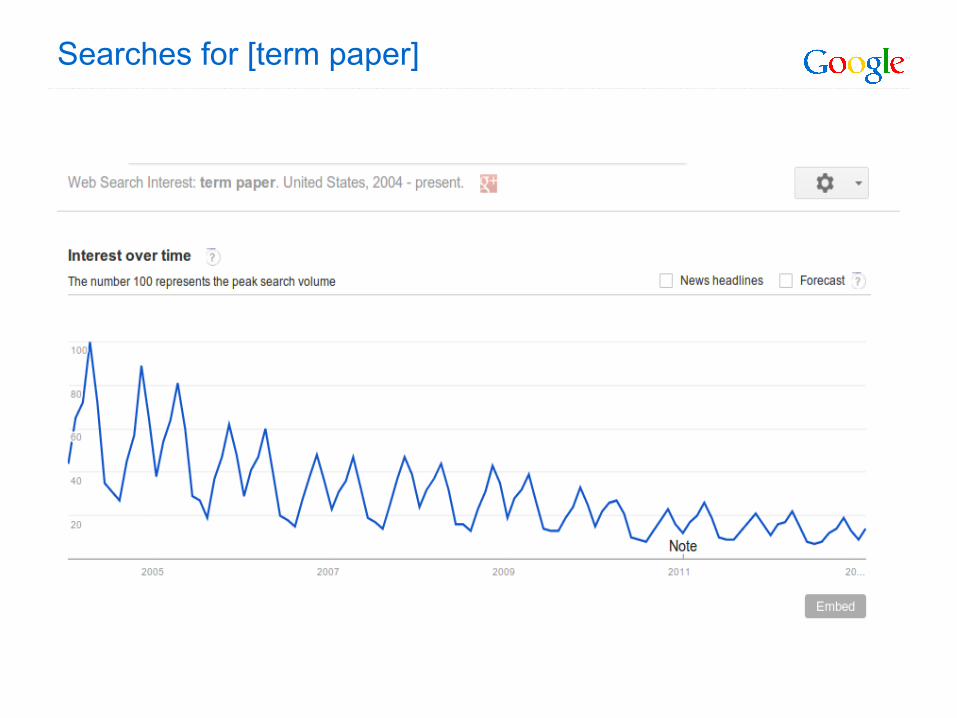
Searches for [term paper]
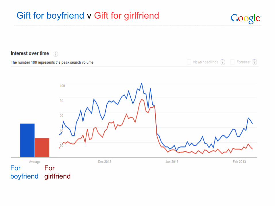
Gift for boyfriend v Gift for girlfriend
Forboyfriend
For girlfriend

Gift for husband v Gift for wife
Forhusband
For wife

12
Google Trends
Google Correlate
Google Consumer Surveys

Searches correlated with [weight loss]
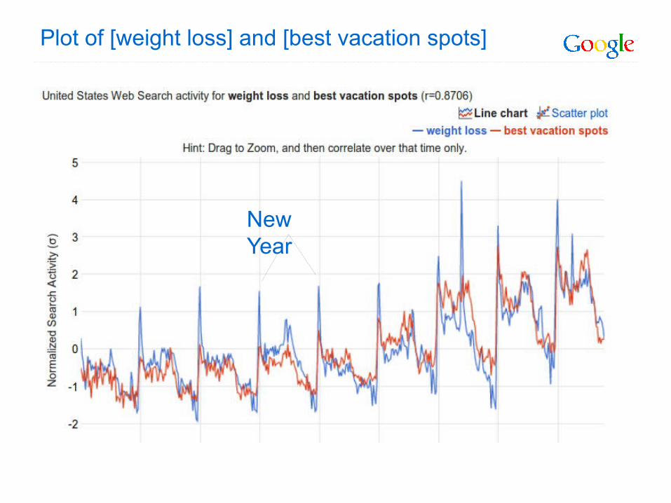
Plot of [weight loss] and [best vacation spots]
New Year

Correlated with [weight loss] 3 weeks later
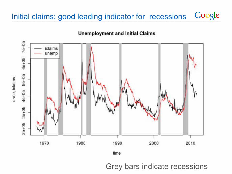
Initial claims: good leading indicator for recessions
Grey bars indicate recessions
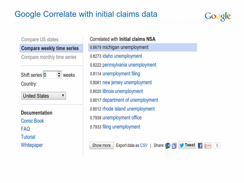
Google Correlate with initial claims data

Initial claims and [unemployment filing]
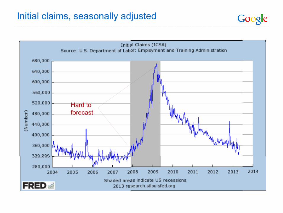
Initial claims, seasonally adjusted
Hard to forecast

Regression models
Baseline model yt = a yt-1 + c + et gives an in-sample MAE of 3.1%
Adding the “unemployment filing” query yt = a yt-1 + b qt + c + et gives an in-sample MAE of 3.0%
Train using t weeks, forecast t+1 (rolling window forecast)MAE of baseline = 3.2%, MAE with query = 3.2%, 0% improvement
During recession MAE of baseline = 3.7%, MAE with query = 3.3%, 8.7% improvement

Gun sales background check

NICS time series
[stack on] has highest correlation[gun shops] is chosen by BSTS

Trend

Seasonal

[gun shops]

Searches on [gun shop]

Our goal: automate model discovery
Challenge 1: spurious correlation
Sometimes find correlations due simply to common seasonality or trend
Challenge 2: fat regression
With more predictors than observations can always find a good fit
Challenge 3: overfitting
Within sample fits typically look better than out of sample fits
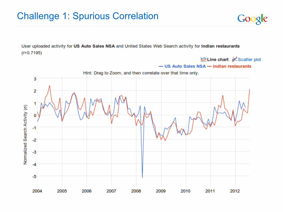
Challenge 1: Spurious Correlation

Challenge 2: Fat regression
Slim regression Fat regression
bXy = = bXy
Any square subset of regressors will fit perfectly
=y= b1X1y b
2X2== b
1X1
b1X1
A subset of regressors might fit well by chance
b1X1

Our approach
Estimating time series: use Kalman filter techniques
Express time series as trend + seasonal + noise (“basic structural model”)
Forecast univariate model using Kalman filter
Advantages: flexibility, adaptive, interpretable, handles non-stationarity well
Model selection using “spike and slab” Bayesian regression
Spike: prior probability that coefficient is included in regression
Slab: diffuse prior for coefficient, conditional on inclusion
Estimate a posterior probability that variable is in model
Combines well with Kalman techniques
Final forecast is weighted average of many models, with weights given by posterior probabilities (Bayesian model averaging)
Example of “ensemble estimation”
Agnostic with respect to “true model”
Tends to avoid overfitting by avoiding choice of “best” single model

Checklist
Kalman filter: handles seasonality and trend
Spike and slab: handles variable selection
Model averaging: averages over many small models to avoid overfitting

UM consumer sentiment index
Monthly data from University of Michigan survey
Select predictors using spike and slab from 157 Google economic verticals, using average value for first 2-weeks of month (about 3 weeks before data is released).
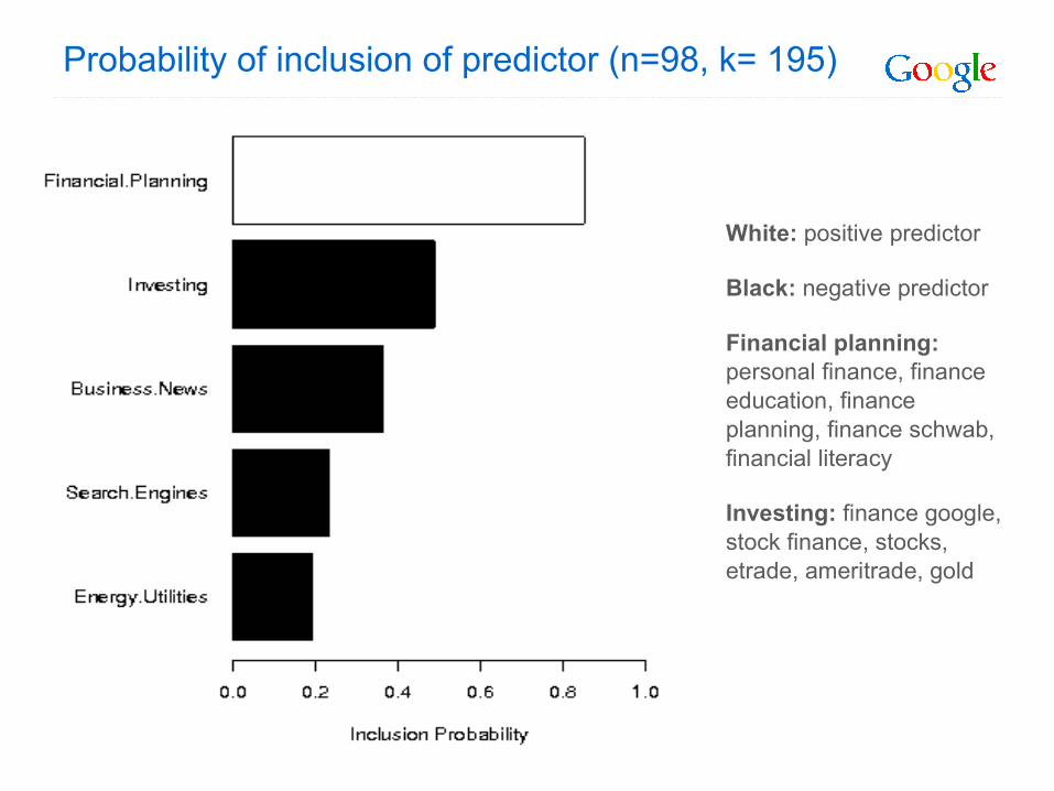
Probability of inclusion of predictor (n=98, k= 195)
White: positive predictor
Black: negative predictor
Financial planning: personal finance, finance education, finance planning, finance schwab, financial literacy
Investing: finance google, stock finance, stocks, etrade, ameritrade, gold
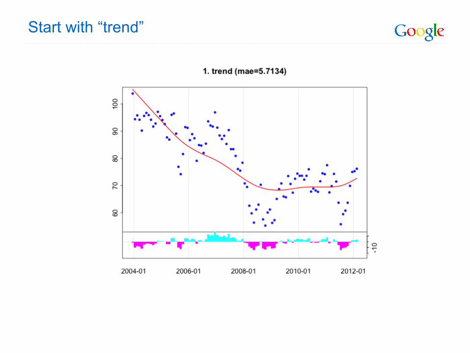
Start with “trend”

Add “financial planning”
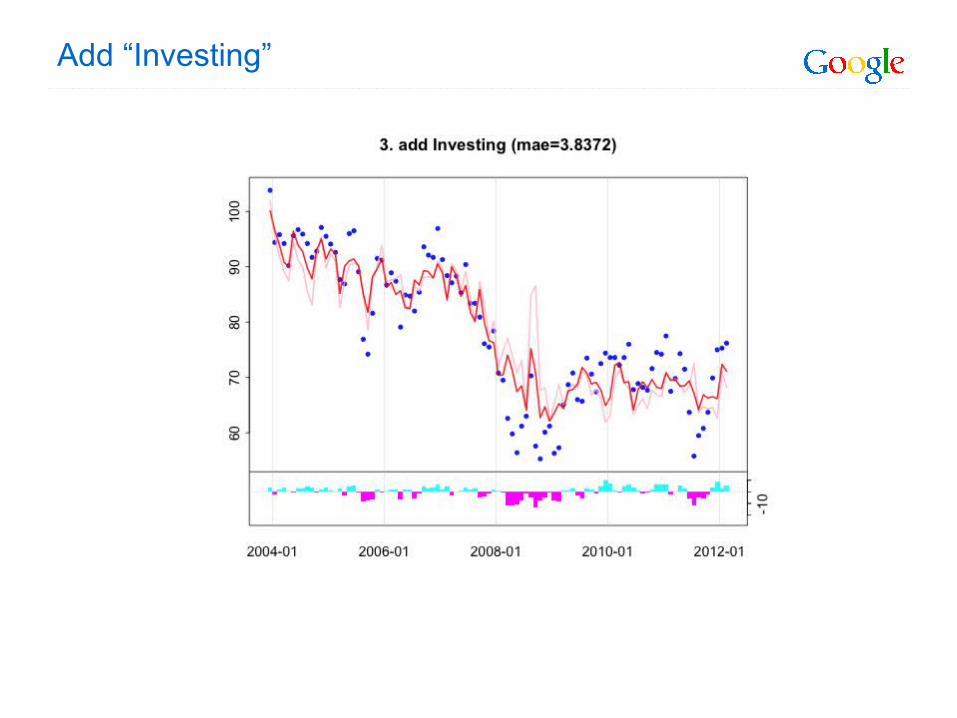
Add “Investing”
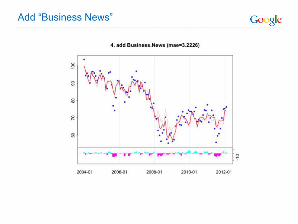
Add “Business News”

Add “Search Engines”
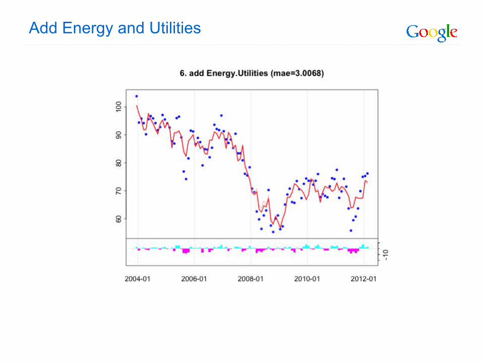
Add Energy and Utilities

40
Google Trends
Google Correlate
Google Consumer Surveys

41
How it works
42

43

44
45
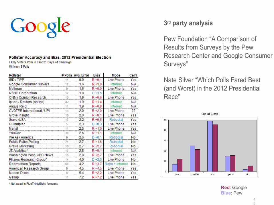
3rd party analysis
Pew Foundation “A Comparison of Results from Surveys by the Pew Research Center and Google Consumer Surveys”
Nate Silver “Which Polls Fared Best (and Worst) in the 2012 Presidential Race”
Red: GoogleBlue: Pew

46
How this changes surveys
Anyone can do them
The cost is dramatically lower
Results come back in a few hours
Surveys can be replicated … or not
You can detect sensitivity due to wording

Challenges for the future
Private sector has high-frequency, real time data and a lot of it!
Visa, Mastercard, American Express
UPS and FedEx
Wal-Mart, Target, etc
Supermarket scanner data
Search engines
Government agencies
Long historical series, but usually low frequency
Carefully constructed but labor intensive, with delayed release and periodic revisions
How to combine the public and private data?
How to integrate massive amounts of private sector real-time information with traditional government statistics


