
1
GPRs Team York University 4700 Keele St. Toronto, ON M3J 1P3 http://www.shareefs.net/gprs
April 30, 2007 Prof. Eshrat Arjomandi Dept. of Computer Science and Engineering Room 2043 CSEB 4700 Keele St. Toronto, ON M3J 1P3 Dear Dr. Arjomandi, Enclosed is the final report of our project outlining the final prototype design of the “Ground Penetrating System” in requirement for the final year Engineering Design course. The report includes a brief background, objectives, technical specifications and final budget for the project. The purpose of the Ground Penetrating System (GPRS) is to use the RADAR techniques to detect ice and water on Martian subsurface. This project gave us an opportunity to demonstrate our engineering knowledge and project management skills in a realistic engineering design environment. We await your comment on the report. Sincerely, The GPRs Team: Amee Shah Azher Shareef Kartheephan Sathiyanathan Nimalraj Navarathinam Enclosure: Final Project Report

YORK UNIVERSITY FACULTY OF SCIENCE AND ENGINEERING
April 30, 2007
GROUND PENETRATING RADAR SYSTEM
Final Project Report
Prepared for:
Dr. ESHRAT ARJOMANDI
In requirement of the course
ENG 4000 ENGINEERING PROJECT
Project Advisor:
Dr. BRENDAN (BEN) QUINE
Prepared By:
GROUP #8
www.shareefs.net/gprs
Amee Shah 207 075 419 [email protected] Azher Shareef 206 686 315 [email protected]
Kartheephan Sathiyanathan 206 762 975 [email protected] Nimalraj Navarathinam 206 727 200 [email protected]

ACKNOWLEDGEMENTS
We would like to convey a special thank you to Dr. Ben Quine in taking time to be our
project advisor and to guide us throughout the project.
We would also like to specially thank Bradley McInnis of the Physics Department and Sasha
Novikov of the Earth and Space Science Department at York University for graciously
lending their extensive time, equipment and expertise. We would also want to thank Harvey
Emberley, Technologist at York University for helping us build the antennas. We would also
like to thank Gillian Moore and Ulya Yigit for helping us with the ordering of project
components and various parts. This project would not have been possible without the active
support of the team members who put up with each other as professional engineers.
Finally, we would like to thank Dr. Eshrat Arjomandi for encouraging and motivating us to
do our best on this project.
ABSTRACT
This document delivers the final design of the Ground Penetrating Radar System (GPRS)
developed by a team of undergraduate space engineering students at York University in
requirement for their final year thesis project. The objective of the GPRS is to detect ice and
water on the Martian subsurface up to a depth of few meters with a resolution of less than a
meter. This report documents the technical specifications of the terrestrial RADAR (Radio
waves Detection and Ranging) system developed and the details of the LabVIEW software
programmed for data acquisition and signal processing. In addition to the testing strategies
used, this document also presents the obstacles encountered during the course of the project,
the final budget and future modifications that can be implemented to improve the systems
performance and utility.

TABLES OF CONTENTS
Acknowledgements ................................................................................................................... 3 Abstract ..................................................................................................................................... 4 1 Introduction ....................................................................................................................... 6
1.1 Background ............................................................................................................... 6
1.2 Objectives.................................................................................................................. 6
2 Technical Theory............................................................................................................... 8
2.1 Frequency Modulated Continuous Wave Radar........................................................ 8
2.2 Implementing The Fmcw System ........................................................................... 10
2.3 Generating Modulation Frequency.......................................................................... 11
2.4 Antenna Design ....................................................................................................... 14
2.5 Structure .................................................................................................................. 16
2.6 Power....................................................................................................................... 17
3 Signal Processing ............................................................................................................ 18
3.1 Sampling.................................................................................................................. 18
3.2 Post Processing........................................................................................................ 19
4 Testing And Results......................................................................................................... 21
4.1 Testing With Transmission Cables .......................................................................... 21
4.2 Testing With Whip Antenna .................................................................................... 22
4.3 Testing With Spiral Antennas .................................................................................. 23
5 Environment, Health And Safety .................................................................................... 25 6 Final Budget .................................................................................................................... 29 7 Future Work..................................................................................................................... 31
7.1 Improvements – Shielding ...................................................................................... 31
7.2 Improvements To The Structure .............................................................................. 32
7.3 Improvements In Signal Processing........................................................................ 32
8 Conclusion....................................................................................................................... 33 9 References ....................................................................................................................... 34 Appendices .............................................................................................................................. 36
Appendix A – Link Budget ................................................................................................. 36
Appendix B – Vco Specifications ....................................................................................... 38
Appendix C – Final System ................................................................................................ 38

6
1 INTRODUCTION
1.1 BACKGROUND
Mars has been at the forefront of several current interplanetary space missions. From the
first successful Mariner 4 mission to the future Phoenix mission in 2007, the search for water
has occupied the scientific community for decades. Being able to find and extract water on
the surface of Mars would allow for successful manned missions to last over extended
periods of time.
Radar techniques are currently used to explore subsurface features on Mars from orbit. These
systems however are limited in terms of resolution and cannot accurately find locations of
buried objects. For future manned mission to Mars, the ability to locate and extract
subsurface ice is vital to the success of the mission. The need for higher resolution detection
is fulfilled by a ground based radar system, such as the GPRS.
Previous Mars missions have shown that water once flowed on the surface of Mars. Current
opinion holds that much of the water has been captured and held under the surface in the
form of ice. In order to be able to extract this trapped water, the source’s location must first
be known.
The GPR system employs a non-invasive method in helping to detect sub-surface water
features. By having the GPR system mounted on a rover, a better resolution of the
subsurface is obtained. This increases the accuracy of pinpointing the locations of boundary
features. This document describes the technical details of the final prototype and also reflects
the engineering strategy used in designing and building the working model. It also outlines
the final budget and possible improvements to the project.
1.2 OBJECTIVES
The primary objective is to design and construct a ground based radar system to detect
subsurface ice and water on Mars for extraction and use by future manned missions. The
system needs to be compact, modular and fully mobile so it may be mounted on a rover.

7
While the final prototype is calibrated to be used on Earth, all the components i.e. the system
as a whole, is designed to be adaptable to the Martian environment.
The secondary objective is to perform real time data acquisition and obtain a visual
representation of the subsurface layer using various signal processing techniques.
An initial constraint was established by the advisor on the frequency requirements for the
radiated signal to be 500 MHz. As a result a large bandwidth was required in order to attain a
better resolution. The size of the antenna was constrained to be within 50 cm so it was
possible to mount it on a rover.
8
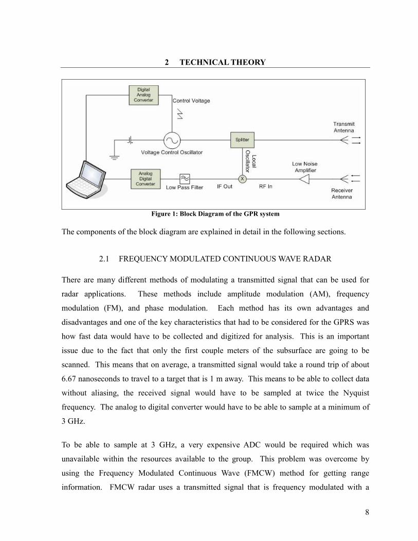
2 TECHNICAL THEORY
Figure 1: Block Diagram of the GPR system
The components of the block diagram are explained in detail in the following sections.
2.1 FREQUENCY MODULATED CONTINUOUS WAVE RADAR
There are many different methods of modulating a transmitted signal that can be used for
radar applications. These methods include amplitude modulation (AM), frequency
modulation (FM), and phase modulation. Each method has its own advantages and
disadvantages and one of the key characteristics that had to be considered for the GPRS was
how fast data would have to be collected and digitized for analysis. This is an important
issue due to the fact that only the first couple meters of the subsurface are going to be
scanned. This means that on average, a transmitted signal would take a round trip of about
6.67 nanoseconds to travel to a target that is 1 m away. This means to be able to collect data
without aliasing, the received signal would have to be sampled at twice the Nyquist
frequency. The analog to digital converter would have to be able to sample at a minimum of
3 GHz.
To be able to sample at 3 GHz, a very expensive ADC would be required which was
unavailable within the resources available to the group. This problem was overcome by
using the Frequency Modulated Continuous Wave (FMCW) method for getting range
information. FMCW radar uses a transmitted signal that is frequency modulated with a
9
certain periodicity. The inverse of this periodicity is known as the modulation frequency.
The modulation frequency is given as:
02
1
tfm = [1]
The rate of frequency change, f& , is given as:
fft
ff m∆=
∆= 2
0
& [2]
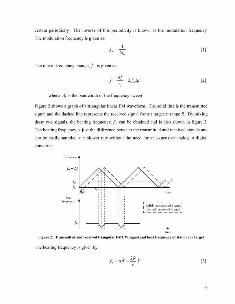
where ∆f is the bandwidth of the frequency sweep Figure 2 shows a graph of a triangular linear FM waveform. The solid line is the transmitted
signal and the dashed line represents the received signal from a target at range R. By mixing
these two signals, the beating frequency, fb, can be obtained and is also shown in figure 2.
The beating frequency is just the difference between the transmitted and received signals and
can be easily sampled at a slower rate without the need for an expensive analog to digital
converter.
Figure 2: Transmitted and received triangular FMCW signal and beat frequency of stationary target
The beating frequency is given by:
fc
Rftfb
&&2
=∆= [3]
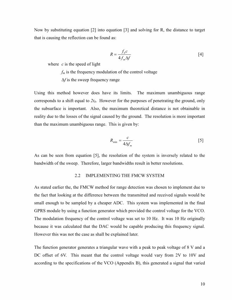
10
Now by substituting equation [2] into equation [3] and solving for R, the distance to target
that is causing the reflection can be found as:
ff
cfR
m
b
∆=4
[4]
where c is the speed of light
fm is the frequency modulation of the control voltage
∆f is the sweep frequency range
Using this method however does have its limits. The maximum unambiguous range
corresponds to a shift equal to 2t0. However for the purposes of penetrating the ground, only
the subsurface is important. Also, the maximum theoretical distance is not obtainable in
reality due to the losses of the signal caused by the ground. The resolution is more important
than the maximum unambiguous range. This is given by:
mf
cR
∆=4
min [5]
As can be seen from equation [5], the resolution of the system is inversely related to the
bandwidth of the sweep. Therefore, larger bandwidths result in better resolutions.
2.2 IMPLEMENTING THE FMCW SYSTEM
As stated earlier the, the FMCW method for range detection was chosen to implement due to
the fact that looking at the difference between the transmitted and received signals would be
small enough to be sampled by a cheaper ADC. This system was implemented in the final
GPRS module by using a function generator which provided the control voltage for the VCO.
The modulation frequency of the control voltage was set to 10 Hz. It was 10 Hz originally
because it was calculated that the DAC would be capable producing this frequency signal.
However this was not the case as shall be explained later.
The function generator generates a triangular wave with a peak to peak voltage of 8 V and a
DC offset of 6V. This meant that the control voltage would vary from 2V to 10V and
according to the specifications of the VCO (Appendix B), this generated a signal that varied
11
in frequency from 300MHz to 450MHz. Therefore, the sweep bandwidth ∆fm is 150MHz
and by using equation [5], the minimum detectable distance is 0.5m.
It is possible to improve the resolution even further to 0.33m by sweeping over the whole
frequency range provided by the VCO. However, other components of the GPRS system
were not compatible with the larger bandwidth. By utilizing the range from 300MHz to
450MHz, the VCO was generating a signal that had the maximum power output as can be
seen from its specification sheets in Appendix B.
2.3 GENERATING MODULATION FREQUENCY
A simple approach to creating a modulation signal is to use a function generator. However
most function generators are large and require a wall outlet. Since a primary goal of the
project was for the system to be mobile, an alternate design was created. This solution
involved creating the modulation signal on a laptop using LabVIEW as the software interface
and sending it through a data acquisition (DAQ) module to a digital to analog (D/A) chip.
The specific DAQ used was the USB-1208FS from Measurement Computing (figure 10).
The first step was to configure the digital input/output (DIO) ports to output data. There are
two ports each with eight bits. Thus ideally the digital signal would have a 16-bit resolution.
However the D/A chip only accepted 12 bits and thus, four bits on the DAQ were not used.
The next step involved sending the appropriate signals to the pins of the D/A. The control
voltages were supplied and the appropriate pins were grounded. Also, one could specify the
range of the D/A chip by making the appropriate connections. For example, in our case, we
make the range 0 V to 10 V where 0 V corresponds to a binary bit pattern of 000000000000
and 10 V corresponds to a binary bit pattern of 111111111111. Also, there were four logical
AND gates which controlled when to latch the incoming digital signals at the 12 input pins.
The most important signal was the chip select signal (CS) which could be toggled to latch
data. Thus one of the DIO bits of the DAQ was connected to the CS pin on the D/A. Then, 12
other bits on the DAQ were connected to the inputs on the D/A.
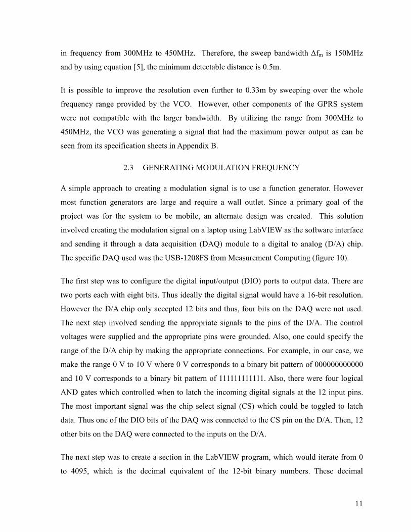
The next step was to create a section in the LabVIEW program, which would iterate from 0
to 4095, which is the decimal equivalent of the 12-bit binary numbers. These decimal
12
numbers were converted into 12 binary bits, which were supplied to the 12 DIO bits using a
function to interact with the DAQ. It was very important to connect the Least Significant Bit
(LSB) outputted by the DAQ to the appropriate pin on the D/A. It was also very important
that the analog signal outputted by the D/A look very smooth and linear since our design is a
linear frequency modulated CW radar. The resolution of the output signal is 10 V divided by
4096, which is 2.441 mV. The frequency of the outputted signal is determined by the rate,
250 Hz, at which the DAQ sends its bits. This limitation of the DAQ prevented the signal
from achieving the desired frequency of 10 Hz as the output rate was required to be 4096 Hz.
Figure 3 - Ramp function obtained using DAQ module
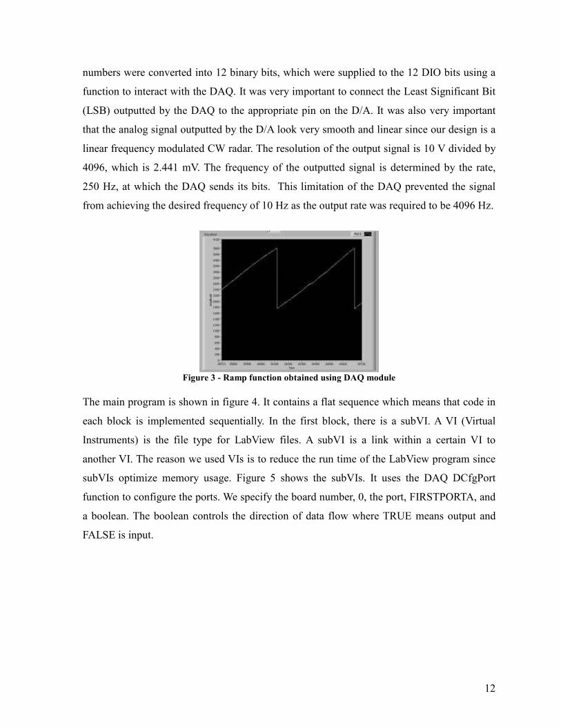
The main program is shown in figure 4. It contains a flat sequence which means that code in
each block is implemented sequentially. In the first block, there is a subVI. A VI (Virtual
Instruments) is the file type for LabView files. A subVI is a link within a certain VI to
another VI. The reason we used VIs is to reduce the run time of the LabView program since
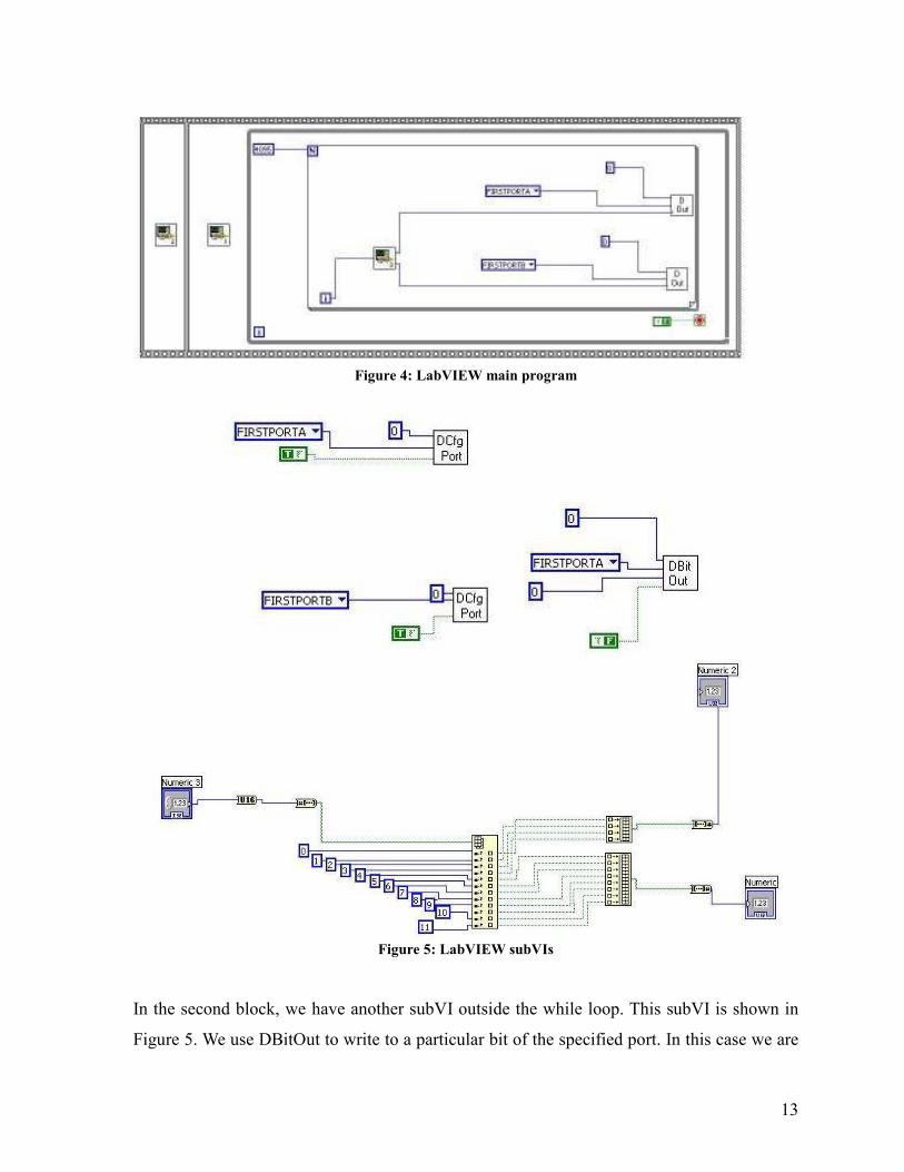
subVIs optimize memory usage. Figure 5 shows the subVIs. It uses the DAQ DCfgPort
function to configure the ports. We specify the board number, 0, the port, FIRSTPORTA, and
a boolean. The boolean controls the direction of data flow where TRUE means output and
FALSE is input.
13
Figure 4: LabVIEW main program
Figure 5: LabVIEW subVIs
In the second block, we have another subVI outside the while loop. This subVI is shown in
Figure 5. We use DBitOut to write to a particular bit of the specified port. In this case we are

14
outputting FALSE from bit 0 of FIRSTPORTA. This is connected to the control signal that
we wish to toggle so that we can latch the information onto the D/A chip. We want the
control signal to be high but since the chip uses negative logic, we need to supply FALSE.
Typically this bit would need to be toggled high and low repeatedly but in this case it was
sufficient to simply set the control signal once and the D/A latched continuously.
Finally, inside the while loop we have a for-loop which iterates from 0 to 4095. Each decimal
value is supplied to a third subVI which breaks the decimal into two decimals. One of the
outputted decimals represents the lower four bits of the original decimal while the second
outputted decimal represents the remaining eight bits. To convert the decimal to binary, the
subVI, shown in Figure 5, extracts the 12 bits associated with the decimal and splits it into
one group of four and another group of eight. The reason for this is because each digital port
on the DAQ only has eight bits. The array with the four bits is passed to FIRSTPORTA using
DOUT in the main program. The remaining eight bits are passed to FIRSTPORTB, also
using DOUT.
2.4 ANTENNA DESIGN
The original design for the GPRS was to use dipole antennas due to its small, compact size
and affordability. However, the antenna was redesigned to have a larger bandwidth to
account for the FMCW method. The dipole antenna commercially available had a very small
bandwidth in the range of 40MHz. The antennas that had the required bandwidth either cost
too much (upwards of $1000) or were too large (greater than 10m).
The GPRS system that was implemented had two antennas, a transmitting and a receiving.
These antennas had to have the capability of being able to work over a large frequency range
and also be affordable. Most importantly, the antennas had to be no larger then 50cm as set
out by the initial requirements so that it can be mounted onto a portable system. To meet
these requirements within budget, equiangular planar spiral antennas were constructed.
Equiangular planar spiral antennas are flat and are frequency independent whose radiation
pattern, impedance and polarization remain unchanged over a large bandwidth. The planar
spiral antenna was chosen because it was flat and circularly polarized. If linear polarized
15
antennas were used, then the strength of the reflected signal would depend on the azimuthal
position of the antennas relative to the object. Also if the orientation of the transmitting and
receiving antennas is orthogonal, the mutual coupling between the two linearly polarized
antennas will be reduced.
The antennas were designed using the equations for r1 (the inner radius) and r2 (the outer
radius):
r1 = r0e
aθ r2 = r0e
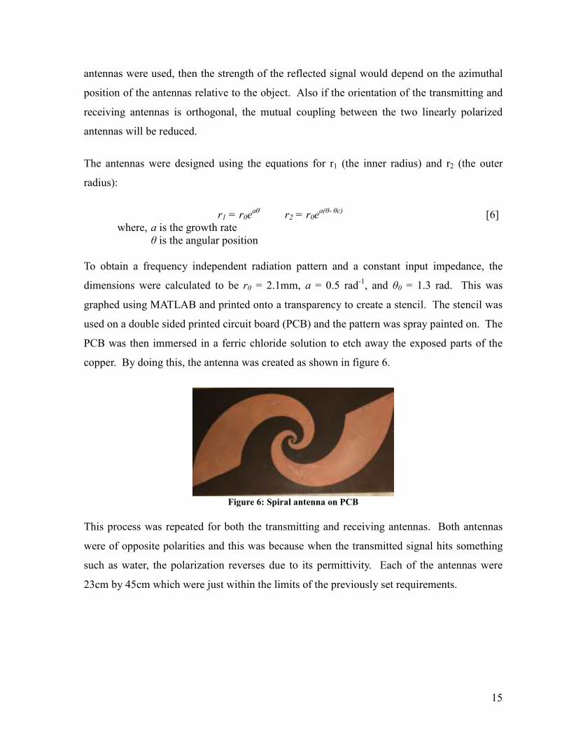
a(θ- θc) [6] where, a is the growth rate θ is the angular position To obtain a frequency independent radiation pattern and a constant input impedance, the
dimensions were calculated to be r0 = 2.1mm, a = 0.5 rad-1, and θ0 = 1.3 rad. This was
graphed using MATLAB and printed onto a transparency to create a stencil. The stencil was
used on a double sided printed circuit board (PCB) and the pattern was spray painted on. The
PCB was then immersed in a ferric chloride solution to etch away the exposed parts of the
copper. By doing this, the antenna was created as shown in figure 6.
Figure 6: Spiral antenna on PCB
This process was repeated for both the transmitting and receiving antennas. Both antennas
were of opposite polarities and this was because when the transmitted signal hits something
such as water, the polarization reverses due to its permittivity. Each of the antennas were
23cm by 45cm which were just within the limits of the previously set requirements.
16
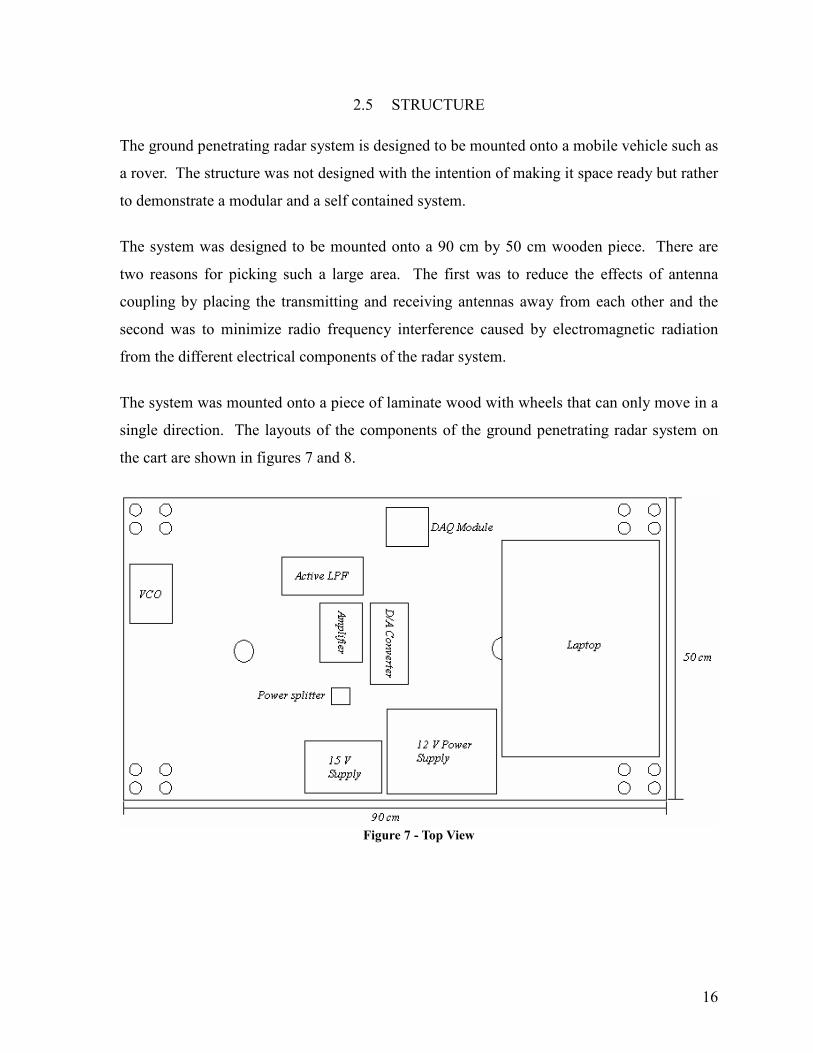
2.5 STRUCTURE
The ground penetrating radar system is designed to be mounted onto a mobile vehicle such as
a rover. The structure was not designed with the intention of making it space ready but rather
to demonstrate a modular and a self contained system.
The system was designed to be mounted onto a 90 cm by 50 cm wooden piece. There are
two reasons for picking such a large area. The first was to reduce the effects of antenna
coupling by placing the transmitting and receiving antennas away from each other and the
second was to minimize radio frequency interference caused by electromagnetic radiation
from the different electrical components of the radar system.
The system was mounted onto a piece of laminate wood with wheels that can only move in a
single direction. The layouts of the components of the ground penetrating radar system on
the cart are shown in figures 7 and 8.
Figure 7 - Top View
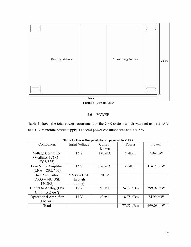
17
Figure 8 - Bottom View
2.6 POWER
Table 1 shows the total power requirement of the GPR system which was met using a 15 V
and a 12 V mobile power supply. The total power consumed was about 0.7 W.
Table 1 : Power Budget of the components for GPRS
Component Input Voltage Current Drawn
Power Power
Voltage Controlled Oscillator (VCO –
ZOS 535)
12 V 140 mA 9 dBm 7.94 mW
Low Noise Amplifier (LNA – ZRL 700)
12 V 520 mA 25 dBm 316.23 mW
Data Acquisition (DAQ – MC USB
1208FS)
5 V (via USB through laptop)
70 µA
Digital to Analog (D/A Chip – AD 667)
15 V 50 mA 24.77 dBm 299.92 mW
Operational Amplifier (LM 741)
15 V 40 mA 18.75 dBm 74.99 mW
Total 77.52 dBm 699.08 mW

18
3 SIGNAL PROCESSING
To acquire the information regarding the target from the incoming received signal, it first
needs to be converted into an intermediate frequency (IF). This is implemented using a
mixer. The transmitted and received signals are mixed to output the signal that will be
processed to retrieve the information about depth and composition of the target. The mixer
output is then passed through a low pass filter to then be sampled by the ADC. The software
then takes the FFT (Fast Fourier Transform) of the sampled signal to acquire the frequency
components, from which the range is determined.
We designed the low pass filter using an operational amplifier as shown in figure 9 with a
cutoff frequency of 25 Hz. We used an active low pass filter rather than a passive one (RC
circuit) because the frequency response (roll off at cut off frequency) for the active low pass
filter was much more accurate.
Figure 9 - Active low lass filter implemented using operational amplifier
1
After the mixed signal is filtered, we sample the signal at a rate of 40 kHz with the analog to
digital converter (ADC) in the DAQ module (USB 1208FS),
3.1 SAMPLING
Although the expected output signal of the mixer in the ground penetrating radar system is
mainly in the range of 10 – 25 Hz, we needed to sample in a significantly higher rate in the
order of kHz because of time constraints. We did not want to sample for long periods with a
slow sampling rate. Instead we chose to sample for shorter periods with a faster sampling
rate. We implemented the sampling using the ADC in a DAQ (data acquisition) module
1 “Lowpass filter”. http://upload.wikimedia.org/wikipedia/commons/7/76/Active_lowpass_filter.svg
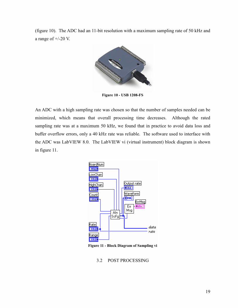
19
(figure 10). The ADC had an 11-bit resolution with a maximum sampling rate of 50 kHz and
a range of +/-20 V.
Figure 10 - USB 1208-FS
An ADC with a high sampling rate was chosen so that the number of samples needed can be
minimized, which means that overall processing time decreases. Although the rated
sampling rate was at a maximum 50 kHz, we found that in practice to avoid data loss and
buffer overflow errors, only a 40 kHz rate was reliable. The software used to interface with
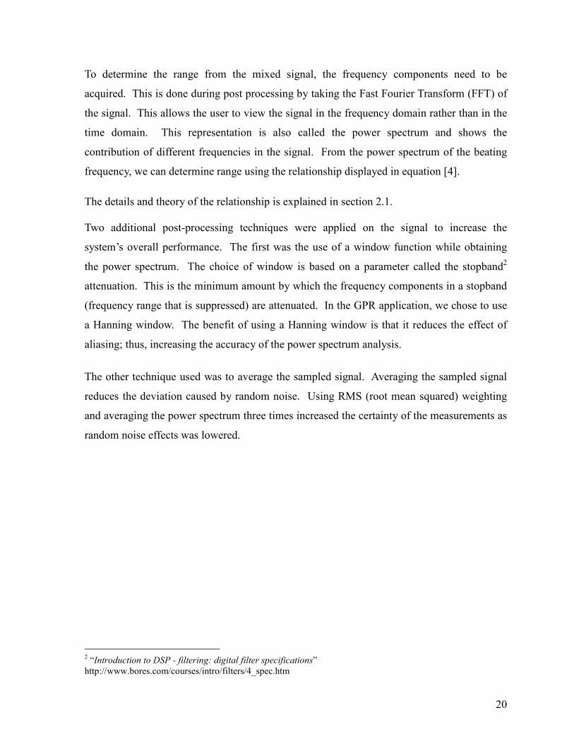
the ADC was LabVIEW 8.0. The LabVIEW vi (virtual instrument) block diagram is shown
in figure 11.
Figure 11 - Block Diagram of Sampling vi
3.2 POST PROCESSING
20
To determine the range from the mixed signal, the frequency components need to be
acquired. This is done during post processing by taking the Fast Fourier Transform (FFT) of
the signal. This allows the user to view the signal in the frequency domain rather than in the
time domain. This representation is also called the power spectrum and shows the
contribution of different frequencies in the signal. From the power spectrum of the beating
frequency, we can determine range using the relationship displayed in equation [4].
The details and theory of the relationship is explained in section 2.1. Two additional post-processing techniques were applied on the signal to increase the
system’s overall performance. The first was the use of a window function while obtaining
the power spectrum. The choice of window is based on a parameter called the stopband2
attenuation. This is the minimum amount by which the frequency components in a stopband
(frequency range that is suppressed) are attenuated. In the GPR application, we chose to use
a Hanning window. The benefit of using a Hanning window is that it reduces the effect of
aliasing; thus, increasing the accuracy of the power spectrum analysis.
The other technique used was to average the sampled signal. Averaging the sampled signal
reduces the deviation caused by random noise. Using RMS (root mean squared) weighting
and averaging the power spectrum three times increased the certainty of the measurements as
random noise effects was lowered.
2 “Introduction to DSP - filtering: digital filter specifications” http://www.bores.com/courses/intro/filters/4_spec.htm
21
4 TESTING AND RESULTS
This section deals with the testing and the results of the GPRS module as it evolved from its
beginning stages. Testing was carried out in three different phases starting with the use of
transmission cables to simulate different lengths, then ¼ wavelength whip antennas and
finally the spiral antennas.
4.1 TESTING WITH TRANSMISSION CABLES
Different length BNC (RF coaxial) cables were used to simulate different target lengths. One
end of the cable was attached to where the transmitting antenna was attached and the other
end was attached to the input of the receiving antenna. This experiment was performed to
verify the theory. The transmission lines thus helped in reducing the external noise produced
by reflections and by other radio signals.
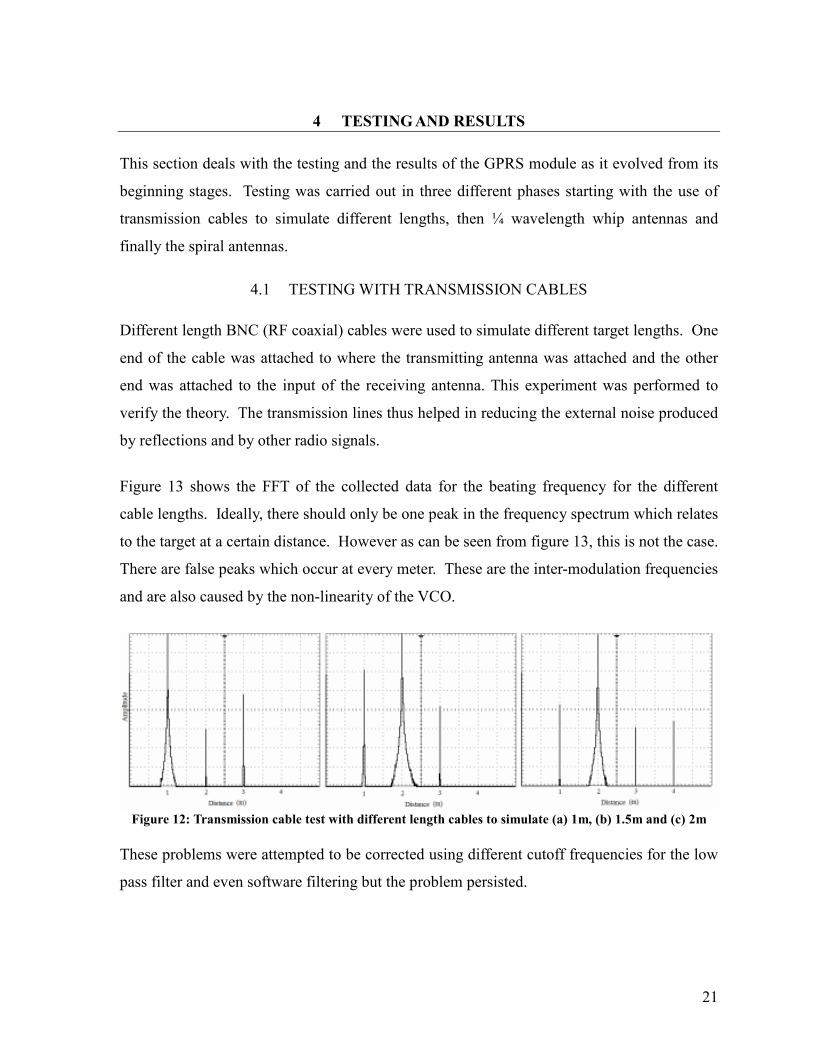
Figure 13 shows the FFT of the collected data for the beating frequency for the different
cable lengths. Ideally, there should only be one peak in the frequency spectrum which relates
to the target at a certain distance. However as can be seen from figure 13, this is not the case.
There are false peaks which occur at every meter. These are the inter-modulation frequencies
and are also caused by the non-linearity of the VCO.
Figure 12: Transmission cable test with different length cables to simulate (a) 1m, (b) 1.5m and (c) 2m
These problems were attempted to be corrected using different cutoff frequencies for the low
pass filter and even software filtering but the problem persisted.
22
Aside from this problem, note how the prominent peak in figure 13a appears at the 1 m mark
for a cable simulating 1 m. In figure 3b, the 1 m peak decreased in amplitude and width,
while the peak at 2 m grew in amplitude and width for a simulation distance of 1.5 m. This
was not initially expected as it was thought that the peak would move to the 1.5 m mark
because the resolution of the system was calculated to be 0.5 m. It was then realized that this
problem was caused by the 10 Hz modulation frequency of the control voltage. Due to the
lack of shielding, the modulation frequency from the function generator was being picked up
by the antenna. This was also seen when changing the modulation frequency. When fm was
changed to 1Hz, the inter-modulation spikes appeared at every 1Hz.
After a lot of testing it was realized that 10Hz for the modulation frequency gave the best
results. Even with the above mentioned two problems, the changes that can be seen in figure
13, as the lengths of the cable varied were quite significant.
4.2 TESTING WITH WHIP ANTENNA
After realizing the limitations of the system from the transmission cable tests, the next step
was to test the system using purchased ¼ wavelength whip antennas. The ¼ wavelength
antennas did not have the required bandwidth of 150MHz. It instead had a bandwidth of
40MHz. Because of this fact, noise due to signal distortion was expected.
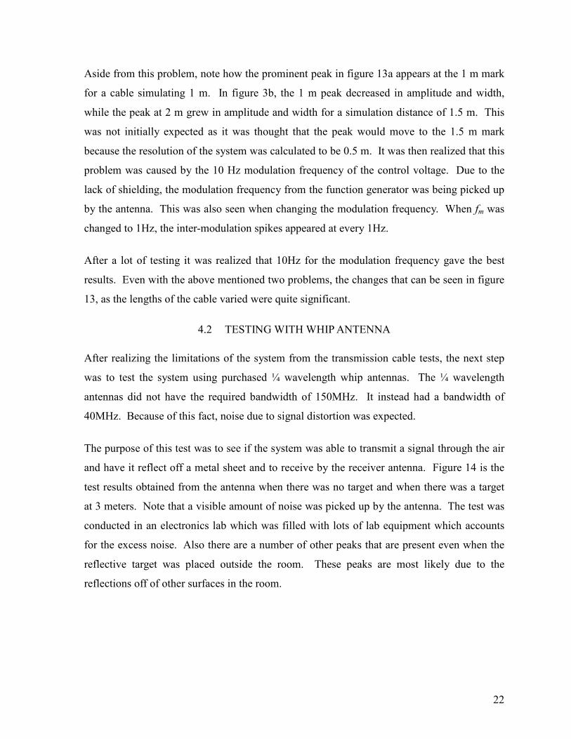
The purpose of this test was to see if the system was able to transmit a signal through the air
and have it reflect off a metal sheet and to receive by the receiver antenna. Figure 14 is the
test results obtained from the antenna when there was no target and when there was a target
at 3 meters. Note that a visible amount of noise was picked up by the antenna. The test was
conducted in an electronics lab which was filled with lots of lab equipment which accounts
for the excess noise. Also there are a number of other peaks that are present even when the
reflective target was placed outside the room. These peaks are most likely due to the
reflections off of other surfaces in the room.
23
Figure 13: Test performed with ¼ wavelength antennas (a) without target and (b) with target at 3m
Other then the excess noise, the change caused by moving the reflective target from outside
the room to 3 meters in front of the antenna pair is clearly visible. The peak at 3m becomes a
lot more prominent in figure 4b than in figure 4a.
4.3 TESTING WITH SPIRAL ANTENNAS
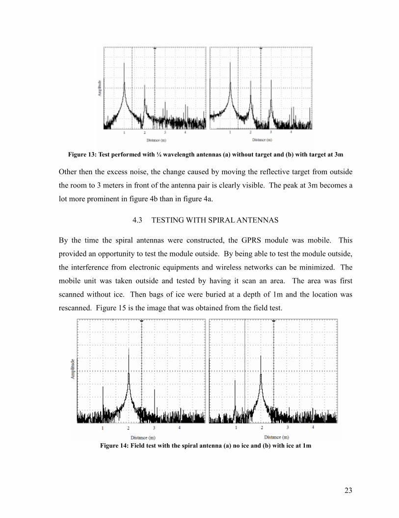
By the time the spiral antennas were constructed, the GPRS module was mobile. This
provided an opportunity to test the module outside. By being able to test the module outside,
the interference from electronic equipments and wireless networks can be minimized. The
mobile unit was taken outside and tested by having it scan an area. The area was first
scanned without ice. Then bags of ice were buried at a depth of 1m and the location was
rescanned. Figure 15 is the image that was obtained from the field test.
Figure 14: Field test with the spiral antenna (a) no ice and (b) with ice at 1m

24
From figure 15a, it can be seen that there is a large spike at the 2m mark. This is most
probably caused by a buried pipe or other objects that are highly reflective. Also note there is
no significant spike at the 1m mark. In figure 15b, a scan was taken when the bags of ice
were buried. As can be seen there is a small change in the spike at the 1 m mark. This
represents the reflection caused by the buried bags of ice.

25
5 ENVIRONMENT, HEALTH AND SAFETY
Anytime we deal with high frequency electromagnetic waves, the question arises if the public
health is at risk. Exposure to Radio Frequency (RF) poses no threat to human health as long
as the power levels are limited [1]. Aside from Ground Penetrating Radar, common
household devices also radiate RF. These devices include the radio, TV, cell and cordless
phones, and Wi-Fi. Moreover, a natural source of RF is the Sun.
The effect of RF on humans is that it causes molecules in tissue to vibrate and generate heat
[2]. If the power level is limited and the RF system is kept below the threshold level, there is
no risk to human health. The threshold level is the amount of exposure required to increase
tissue temperature by at least 1°C [2]. Certain factors significantly reduce human exposure to
RF by a factor of at least 100 [2]. One factor is our directional antenna, which is much better
than an omni-directional antenna. The RF energy is contained in beams and the energy level
outside the main beam is thousands of times lower [2]. Shielding is another factor that can
limit the amount of radiation.
There are safety guidelines for the use of radio frequency fields. The publication, “Limits of
Exposure to Radio Frequency Fields at Frequencies from 10 kHz – 300 GHz”, also known as
Safety Code 6, outlines such guidelines [3]. It states that the risk to health depends on several
factors: strength of the field, exposure duration, frequency, modulation, polarization, and
distance from the source [3]. The rate at which RF electromagnetic energy is absorbed in the
body is known as specific absorption rate (SAR). The unit of SAR is Watts per kilogram.
26
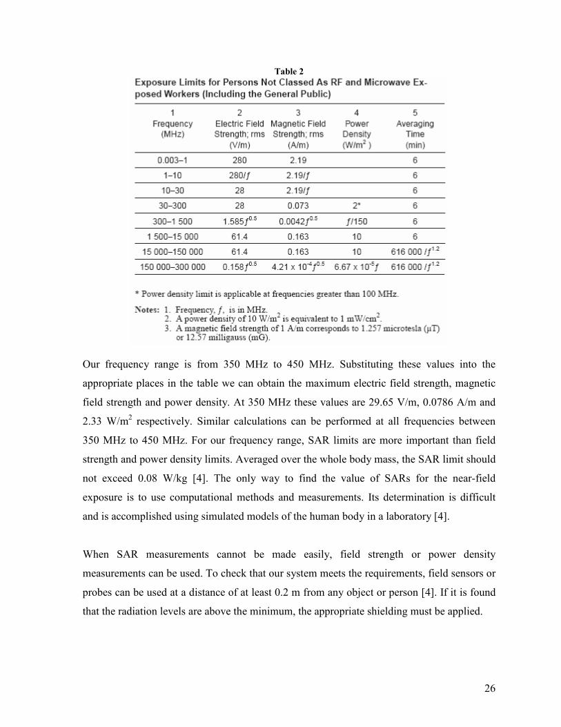
Table 2
Our frequency range is from 350 MHz to 450 MHz. Substituting these values into the
appropriate places in the table we can obtain the maximum electric field strength, magnetic
field strength and power density. At 350 MHz these values are 29.65 V/m, 0.0786 A/m and
2.33 W/m2 respectively. Similar calculations can be performed at all frequencies between
350 MHz to 450 MHz. For our frequency range, SAR limits are more important than field
strength and power density limits. Averaged over the whole body mass, the SAR limit should
not exceed 0.08 W/kg [4]. The only way to find the value of SARs for the near-field
exposure is to use computational methods and measurements. Its determination is difficult
and is accomplished using simulated models of the human body in a laboratory [4].
When SAR measurements cannot be made easily, field strength or power density
measurements can be used. To check that our system meets the requirements, field sensors or
probes can be used at a distance of at least 0.2 m from any object or person [4]. If it is found
that the radiation levels are above the minimum, the appropriate shielding must be applied.

27
We now include sample calculations of the maximum power density [4]. This calculation is
for the near-field zone,
WP
A
where
W
P
A
m
T
m
T
=
=
=
=
4
,
maximum power density (W / m )
net power delivered to the antenna (W)
physical aperture area (m )
2
2
For a net power delivered to the transmitting antenna of 0.00794 W and a physical aperture
area of 0.1035 m2, we obtain a maximum power density of 0.07671 W/m2. In the far-field
region, the power density on the main beam is given by the following expression [4],
WP G
r
where
P
r
G
T
T
=
=
=
=
4 2π
,
net power delivered to the antenna (W)
distance from the antenna (m)
antenna gain with respect to an isotropic antenna
The antenna gain is give by the following expression [4],
GA
where
A A
A
e
e
=
= =
=
= ≤ ≤
=
42
π
λ
ε
ε ε
λ
,
effective area of the antenna, A
physical aperture area of the antenna (m )
antenna efficiency (typically 0.5 0.75)
wavelength (m)
e
2
The expression for the beginning of the far-field region is given by the following expression [4],
rD
where
D
=
=
=
05 2.
,
λ
λ
the greatest dimension of the antenna (m)
wavelength (m)
28
For an antenna efficiency of 0.6, which is the average of the typical efficiency values, and a
wavelength that corresponds to 350 MHz, we obtain a gain of 1.062. Then, for the greatest
antenna dimension of 0.45 m and the same wavelength, we obtain a far-field range of 0.118
m. With the calculated gain and range, we obtain a power density for the far-field of 0.04819
W/m2.
Finally, we calculate the rms electric field strength at the far-field distance [4],
EEIRP
r
where
EIRP G
=
=
[ ]
,
.30 0 5
effective isotropically radiated power (W), EIRP = PT
Using values from previous calculations, we obtain a rms electric field strength at the far-
field distance of 4.262 V/m.
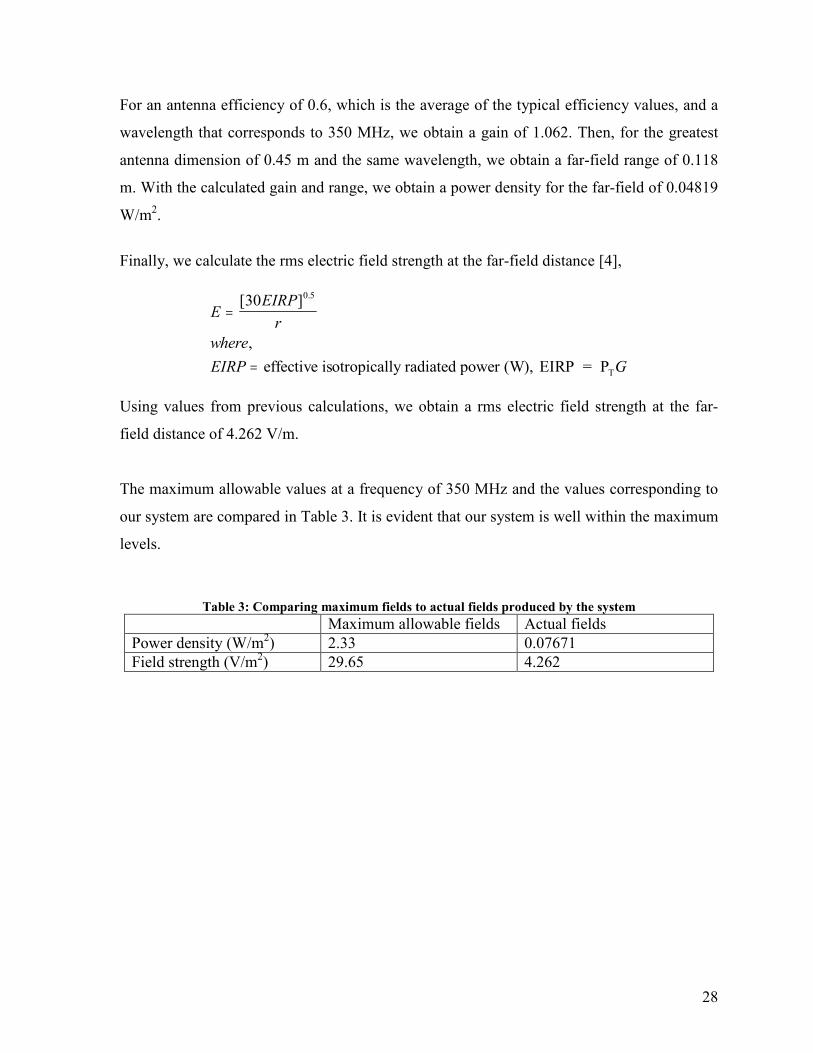
The maximum allowable values at a frequency of 350 MHz and the values corresponding to
our system are compared in Table 3. It is evident that our system is well within the maximum
levels.
Table 3: Comparing maximum fields to actual fields produced by the system
Maximum allowable fields Actual fields
Power density (W/m2) 2.33 0.07671
Field strength (V/m2) 29.65 4.262

29
6 FINAL BUDGET
The final prototype of the Ground Penetrating Radar system was delivered in accordance
with the objectives and the stated requirements. The budgetary constraint of $1000 Canadian
dollars was considered throughout the project. Over the course of the project’s development,
various components were bought as well as borrowed from the facilities at York University.
The initial budget estimate was an approximation based on the initial research and limited
background on the subject. All of the listed prices are in Canadian dollars and they include
tax wherever applicable. Note that any facilities or components of the project that are
available at no charge are not included in this budget summary.
Table 2 shows the budget initially established by the team for the project.
Table 4 – Initial Budget Estimate
Component Cost ($)
Transmitting antenna 50.00
Receiving antenna 50.00
Signal Generator 60.00
Amplifiers 55.00
Mobile Unit 125.00
Sandbox 100.00
Presentation 200.00
Total 640.00
The final budget is listed in table 3.
Table 5 – Final Budget
Components Quantity Unit Price ($) Total Amount ($)
Voltage Controlled Oscillator 1 133.97 133.97
Low Noise Amplifier (LNA) 1 133.97 133.97
Power Splitter 1 27.87 27.87
Mixer 1 54.67 54.67
Dipole Antenna 4 11.81 47.24
D/A Chip 1 19.95 19.95
SMA cables 4 22.76 91.04
SMA Jack 3 5.35 16.05
Subtotal 524.76
Miscellaneous Items Total Amount ($)
Electronic Components (Batteries, Cables, Resistors) 25.31
Velcro 9.09
Wood 15.95
Wheels, Nuts, Bolts 40.05

30
Tub (for etching) 13.67
Poster 60.00
Ice (for Demo) 15.00
Total Shipping 135.37
Subtotal 314.44
Total 839.21
The final budget varied from the initial budget as the project progressed. This was due to the
fact that the special RF (radio frequency) rated components were required to operate at a high
frequency of about 500 MHz. The major components were shipped from Mini-circuits in the
US which contributed to the shipping and handling charges.
31
7 FUTURE WORK
7.1 IMPROVEMENTS – SHIELDING
Our system operates in the Ultra High Frequency (UHF) range, which is from 300 MHz to 3
GHz [1]. The voltage-controlled oscillator (VCO) generates frequencies from 300 MHz to
450 MHz. However, the spiral antennas that we created have a wide bandwidth and receive
signals with frequencies from 300 MHz to 1.3 GHz. Therefore the receiving antenna is
accepting signals from anything that operates in this range. They include television
transmitters, mobile phones, Global Positioning System, AM/FM radio, 2-way radio, paging,
and emergency and public safety communications systems [2]. Another device that uses UHF
frequencies is 802.11b (“Wifi”). All of these things create what is known as radio frequency
interference (RFI). Results of RFI include signal quality degradation and lowered system
performance [2].
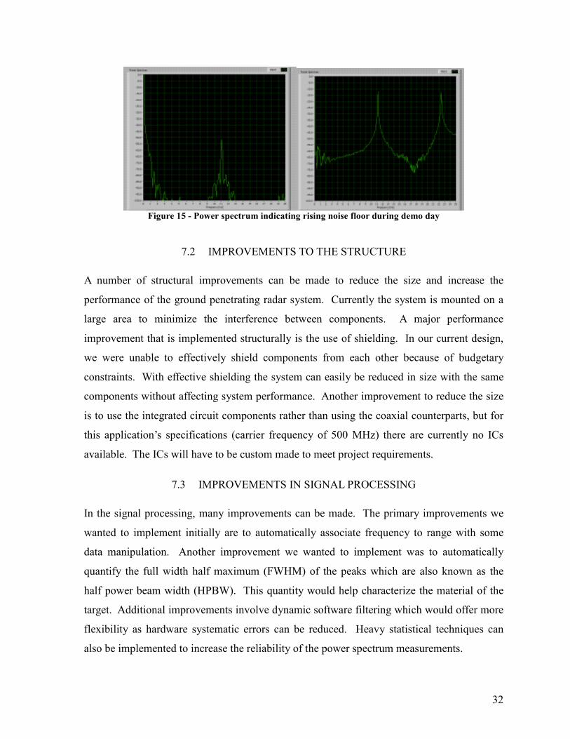
The problem of RFI was experienced during our numerous tests. For example, when testing
in the Petrie Science and Engineering electronics laboratory, the signals were hard to
decipher and were not as we expected. However, similar tests in the basement of the same
building produced better results. This can be explained by the fact that the basement is
relatively free from interference from all the sources aforementioned. Even during the day of
the demonstration, we witnessed an increase in the interference as the day progressed and the
room filled with electronic equipment. The noise floor of our Fast Fourier Transformation
went up by approximately 20 dBm. Numerous other projects were using Wi-Fi, which have
possibly contributed to the interference.
The solution is to use electromagnetic shielding. When this technique is used to block radio
frequency electromagnetic radiation, it is known as RF shielding [3]. Factors that affect the
amount of interference reduced include the type of material used, its thickness and the
frequency involved [3]. Materials that could have been used include sheet metal and metal
meshes.
32
Figure 15 - Power spectrum indicating rising noise floor during demo day
7.2 IMPROVEMENTS TO THE STRUCTURE
A number of structural improvements can be made to reduce the size and increase the
performance of the ground penetrating radar system. Currently the system is mounted on a
large area to minimize the interference between components. A major performance
improvement that is implemented structurally is the use of shielding. In our current design,
we were unable to effectively shield components from each other because of budgetary
constraints. With effective shielding the system can easily be reduced in size with the same
components without affecting system performance. Another improvement to reduce the size
is to use the integrated circuit components rather than using the coaxial counterparts, but for
this application’s specifications (carrier frequency of 500 MHz) there are currently no ICs
available. The ICs will have to be custom made to meet project requirements.
7.3 IMPROVEMENTS IN SIGNAL PROCESSING
In the signal processing, many improvements can be made. The primary improvements we
wanted to implement initially are to automatically associate frequency to range with some
data manipulation. Another improvement we wanted to implement was to automatically
quantify the full width half maximum (FWHM) of the peaks which are also known as the
half power beam width (HPBW). This quantity would help characterize the material of the
target. Additional improvements involve dynamic software filtering which would offer more
flexibility as hardware systematic errors can be reduced. Heavy statistical techniques can
also be implemented to increase the reliability of the power spectrum measurements.
33
8 CONCLUSION
This project gave us an opportunity to use our engineering skills and knowledge gained over
the years to design and build a Ground Penetrating Radar system. We gained a greater
understanding and a more hands on experience with the engineering design process
throughout the completion of the project. After getting acquainted with the RF (radio
frequency) technology, we feel that building a radar system under thin budget and time
constraint is a personal success.
The final product can be expanded on for future projects that could broaden the scope for
finding water on Mars. For example, the rover can be made to be a lot more automated so
that it can go to specified locations with minimal human interaction. Another expansion
would be the possibility of adding an automated drilling system onto the rover. This drilling
system could be used to drill up to a certain depth to extract the water that could be found
using the GPR system. All in all, the possibilities for the ground based GPR system on Mars
are limitless.

34
9 REFERENCES
[1] http://th.physik.uni-frankfurt.de/~hossi/HEALTH_SAFETY_QA.pdf [2] http://www.who.int/mediacentre/factsheets/fs226/en/ [3] http://www.hc-sc.gc.ca/ewh-semt/pubs/radiation/safety-faq-securite_e.html [4] http://www.hc-sc.gc.ca/ewh-semt/alt_formats/hecs-sesc/pdf/pubs/radiation/99ehd-dhm237/99ehd-dhm237_e.pdf [5] Herman, H. “Robotic Subsurface Mapping Using Ground Penetrating Radar”. The Robotics Institute, Carnegie Mellon University. May 1997. [6] Lacomme, P., J. Hardange, J. Marchais and E. Normant. “Air and Spaceborne Radar Systems: An Introduction”. [7] Mahafza, B., “Radar Systems - Analysis and Design Using MATLAB”. Chapman & Hall/Crc. January 2000.
[8] http://www.georadar.com/howitwrk.htm
[9] http://www.gpr-survey.com/
[10] http://www.ece.ucsb.edu/gpr2002/
[11] http://www.g-p-r.com/
[12] http://www.gprmtl.com/
[13] http://www.ldolphin.org/GPRbkgnd.html
[14] http://www.malags.com/
[15] http://www.du.edu/~lconyer/
[16] http://ieeexplore.ieee.org/iel3/5215/14097/00646396.pdf?isnumber=&arnumber=646396
[17] http://www.osti.gov/bridge/servlets/purl/10120066-cu7Id4/native/10120066.pdf
[18] http://www.osti.gov/bridge/servlets/purl/10177821-oaYMME/10177821.PDF
[19] http://cobalt.cneas.tohoku.ac.jp/users/sato/gpr96/Author/Program(Aug8).html

35
[20] http://ieeexplore.ieee.org/iel3/5225/14128/00648553.pdf?arnumber=648553
[21] http://www.iee.org/oncomms/sector/communications/Articles/Object/DF965D14-9AD5-5B6D-6C02C5988751A8A3
[22] http://www.iee.org/oncomms/sector/communications/Articles/Object/1278C8B6-CFAE-4B23-89F269B668E0C8F3
[23] http://www.iee.org/oncomms/sector/communications/Articles/Object/845F1423-D8E7-4A25-B408FF3EBC6A9076
[24] http://huizen.deds.nl/~pa0hoo/helix_wifi/linkbudgetcalc/wlan_budgetcalc.html
[25] http://www.geomodel.com/
[26] http://www.maverickinspection.com/gprfaq.html
[27] http://www.geo-graf.com/gpr-1.htm
[28] http://www.everything2.com/index.pl?node_id=1089803
36
APPENDICES
APPENDIX A – LINK BUDGET
Link Budget for the project was carried out using Matlab. The code is as follows: % GPRS – System Design
% Link Budget
% Frequency f = 500 MHz
f = 500E6; % Hz
% Speed of light in vacuum
c = 3E8; % m/s
% Wavelength in meters
lambda = c/f; % m
% Antenna loss - measure of the power available for radiation as a
% proportion of the power applied to the antenna terminals
Le = -4; %dB for loaded dipole antennas
% Antenna mismatch loss - measure of how well antenna is matched to the
% transmitter
Lm = -1; % dB
% Characteristic impedance of air
Za = 377; % ohms, given in gpr book
% tan(delta)= Im(epsilr)/Re(epsilr): dissipation factor or Loss tangent
% Characteristic impedance of the material
% Zm = (sqrt(mu0*mur/(epsil0*epsilr)))*
(1/(1+tan(delta)^2)^(1/4))*(cos(delta/2)+j*sin(delta/2));
% For earthy materials
Zm = 125 ; % ohms
% Transmission coupling loss - transmission loss from the antenna to the
% material
Lt1 = -20*log(4*Zm*Za/abs(Zm + Za)^2); % dB
% Retransmission coupling loss - from the material to the air on the
return
% journey
Lt2 = -20*log(4*Zm*Za/abs(Zm + Za)^2); % dB
% Gain of transmitting antenna (loaded dipole)
Gt = 3;
% Receiving Aperture
Ar = (0.285)^2; % m^2 (dipole antenna thats 28.5 cm long (assuming A =
0.95))
% Range to the target
R = 3; % in metres (because depth is around 10 ft)
% Radar cross section
sigma = 1; %m^2 (not sure about this) assumed to be unity as the
subsurface resembles an infinitely large dielectric space

37
% Spreading loss - ratio of the received power to the transmitted power
% Ls = -10*log(Gt*Ar*sigma/(4*pi*R^2)^2); % dB from the book
Ls = -10*log((Gt*lambda)^2*sigma/(4*pi*R)^2); % dB from the research paper
% Target Scattering loss
% Z1 = Za; Z2 = Zm;
% Lsc = 20*log(1-abs((Z1-Z2)/(Z1+Z2))) + 20*log(sigma);
Lsc = -1.6; % for typical case when sigma=1
% Material Attenuation loss
% La = 8.686*2*R*2*pi*f*sqrt(mu0*mur*epsil0*epsilr/2*sqrt(1+tan(delta)^2)-
1);
La = -10; % assumption of 10 dB
% Total Path loss (dB)
Lt = Le + Lm + Lt1+Lt2+ Ls + La + Lsc
% Power Budget = sum of TSS, Lt and internal noise
% Tangential Signal Sensitivity (8-dB higher than the noise level Pn)
% External Thermal noise Pn = kTB where B = 1.57f(3dB)
Pn = -74.2; % dBm @ 300 Kelvin for 0-6 GHz receiver
Tss = -74.2+8;
% Internal Noise F is negligible (not significant since the IF bandwidth
is in
% the range of few to several hundred megahertz only
intNoise = 0; % in dB/m
% Power in dBm
PdBm = Tss + Lt + intNoise
% Power in mW
PmW =10^(PdBm/10)
Results:
Power = -10.3491 dBm
Power = 0.0923 mW ~ 0.1 mW
38
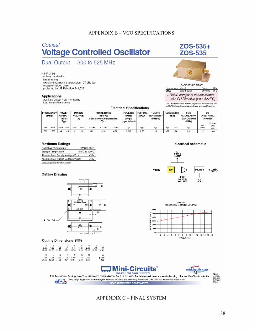
APPENDIX B – VCO SPECIFICATIONS
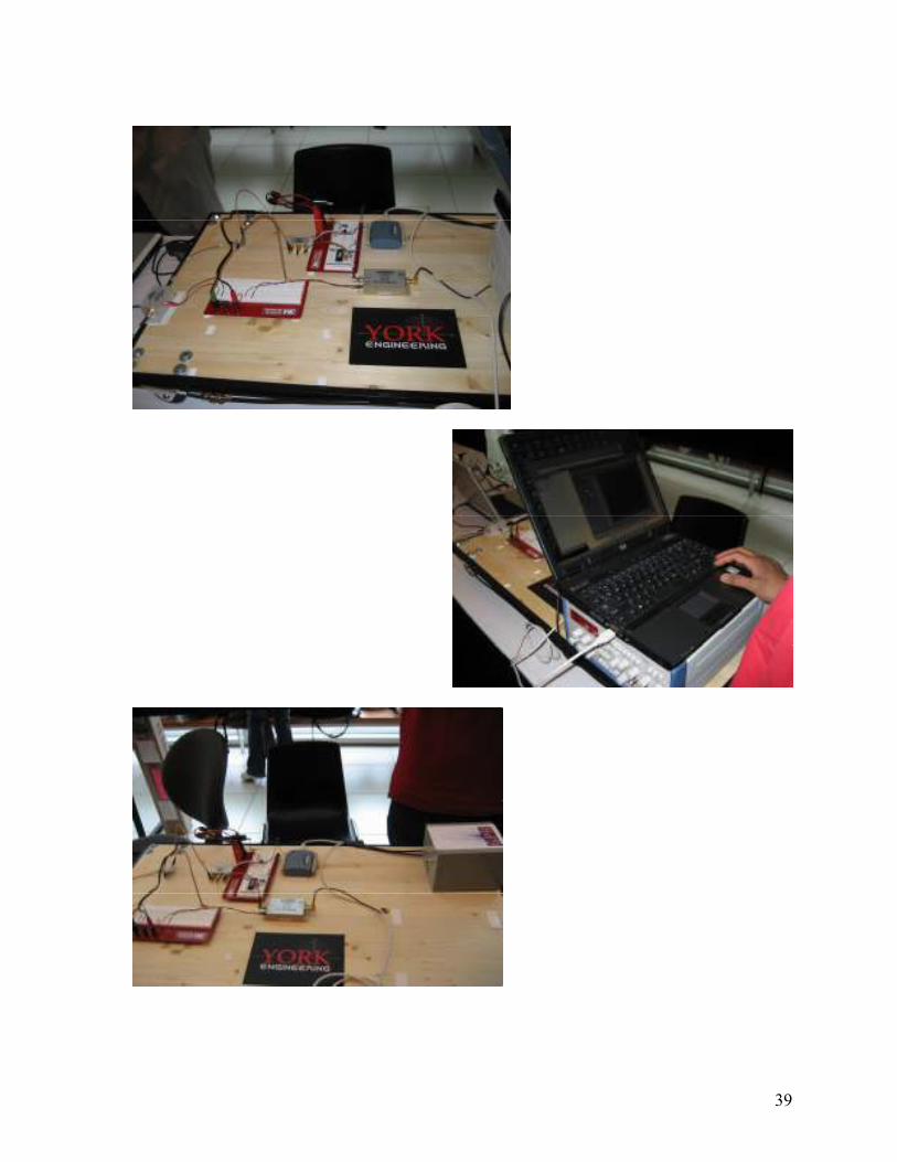
APPENDIX C – FINAL SYSTEM
39


