
GPU-enabled Real-time Risk Pricing in Option Market Making
Cris Doloc, Ph.D.
21st March 2013

Disclaimer
2
The statements, remarks and conclusions of this presentation are my own and they do not represent necessarily the view of CTC
The results presented in this paper are not necessarily related to the work I am currently doing for CTC, nor to the technology or infrastructure employed by CTC
OUTLINE
1. Introduction to Market Making in exchange traded Options
2. Defining the problem: Real-time Pricing of RISK
3. Survey of numerical methods for Option Risk valuation
4. CUDA implementation of accelerated lattice models
Preliminary results & comparative study
5. Potential new developments
6. Conclusions
3
GPU users Ecosystem in finance
Investment Banks– OTC
Insurance companies
Solution Vendors / ISV
Academia
Proprietary Trading Firms
Hedge Funds
4
1. Intro to Options Market Making
5
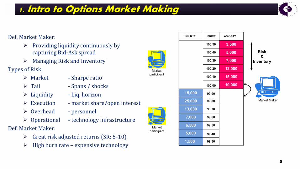
Def. Market Maker:
Providing liquidity continuously by capturing Bid-Ask spread
Managing Risk and Inventory
Types of Risk:
Market - Sharpe ratio
Tail - Spans / shocks
Liquidity - Liq. horizon
Execution - market share/open interest
Overhead - personnel
Operational - technology infrastructure
Def. Market Maker:
Great risk adjusted returns (SR: 5-10)
High burn rate – expensive technology
TECHNOLOGY INFRASTRUCTURE
6
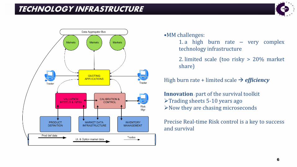
•MM challenges: 1. a high burn rate – very complex technology infrastructure
2. limited scale (too risky > 20% market share)
High burn rate + limited scale efficiency Innovation - part of the survival toolkit Trading sheets 5-10 years ago Now they are chasing microseconds
Precise Real-time Risk control is a key to success and survival
2. Defining the Problem
7
Options on a wide variety of Asset Classes and Geographies
Index : Cash / ETF / Futures
Commodities: Energy / Metals / Agricultural
Fixed Income: entire Yield curve (US and foreign)
Equities: US and foreign
Dimensionality
Large portfolios: +100K products
Complex scenarios: Underlying Prices / Volatility / Events: dividends, credit, political
Real-time requirements - time-scale sub-second
Pricing Risk IN “REAL-TIME”
8
Drivers for Risk system requirements:
REGULATIONS & CORRELATION Risk
High AVAILABILITY through ACURACY/SPEED TIGHTER RISK CONTROL
SCALABILITY across users/prod/geographies COST REDUCTION
TIME SCALE: Real-time vs. Batch
Real Time P&L and basic Greeks (model parameters sensitivities)
Scenarios traditionally in batch mode, but currently RT
RISK VALUATION WORKFLOW
9
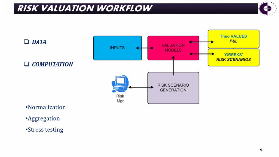
DATA
COMPUTATION
•Normalization
•Aggregation
•Stress testing

Real-time RISK Infrastructure
10
3. Survey of numerical methods for Pricing
11
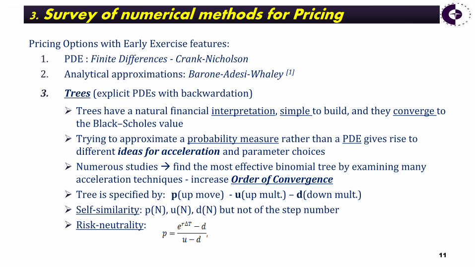
Pricing Options with Early Exercise features:
1. PDE : Finite Differences - Crank-Nicholson
2. Analytical approximations: Barone-Adesi-Whaley [1]
3. Trees (explicit PDEs with backwardation)
Trees have a natural financial interpretation, simple to build, and they converge to the Black–Scholes value
Trying to approximate a probability measure rather than a PDE gives rise to different ideas for acceleration and parameter choices
Numerous studies find the most effective binomial tree by examining many acceleration techniques - increase Order of Convergence
Tree is specified by: p(up move) - u(up mult.) – d(down mult.)
Self-similarity: p(N), u(N), d(N) but not of the step number
Risk-neutrality:
VARIETY OF BINOMIAL TREE MODELS
12
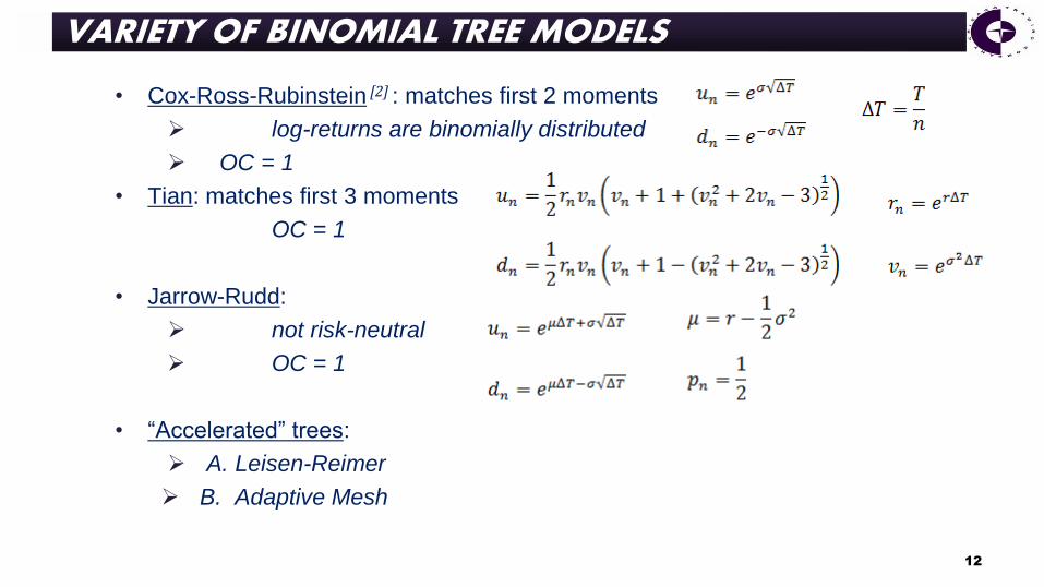
• Cox-Ross-Rubinstein [2] : matches first 2 moments
log-returns are binomially distributed
OC = 1
• Tian: matches first 3 moments
OC = 1
• Jarrow-Rudd:
not risk-neutral
OC = 1
• “Accelerated” trees:
A. Leisen-Reimer
B. Adaptive Mesh
A. Leisen-Reimer TREE
13
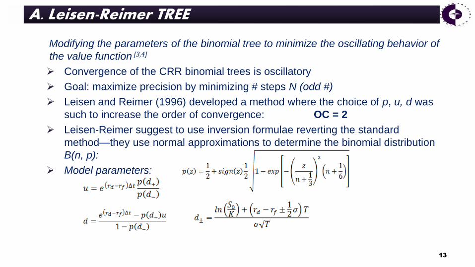
Modifying the parameters of the binomial tree to minimize the oscillating behavior of
the value function [3,4]
Convergence of the CRR binomial trees is oscillatory
Goal: maximize precision by minimizing # steps N (odd #)
Leisen and Reimer (1996) developed a method where the choice of p, u, d was
such to increase the order of convergence: OC = 2
Leisen-Reimer suggest to use inversion formulae reverting the standard
method—they use normal approximations to determine the binomial distribution
B(n, p):
Model parameters:

CRR versus L-R
14
S = 95 K = 100
σ = 25% r = 5%
1 yr
S = 95 K = 100 σ = 25% r = 5% 1 yr
Ways to FURTHER improve convergence
15
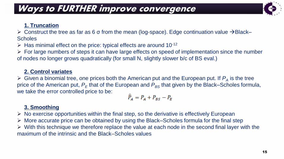
1. Truncation
Construct the tree as far as 6 σ from the mean (log-space). Edge continuation value Black–
Scholes
Has minimal effect on the price: typical effects are around 10-12
For large numbers of steps it can have large effects on speed of implementation since the number
of nodes no longer grows quadratically (for small N, slightly slower b/c of BS eval.)
2. Control variates
Given a binomial tree, one prices both the American put and the European put. If PA is the tree
price of the American put, PE that of the European and PBS that given by the Black–Scholes formula,
we take the error controlled price to be:
3. Smoothing
No exercise opportunities within the final step, so the derivative is effectively European
More accurate price can be obtained by using the Black–Scholes formula for the final step
With this technique we therefore replace the value at each node in the second final layer with the
maximum of the intrinsic and the Black–Scholes values
Richardson Extrapolation
16
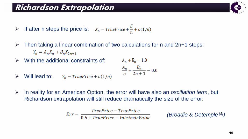
If after n steps the price is:
Then taking a linear combination of two calculations for n and 2n+1 steps:
With the additional constraints of:
Will lead to:
In reality for an American Option, the error will have also an oscillation term, but
Richardson extrapolation will still reduce dramatically the size of the error:
(Broadie & Detemple [5])

B. ADAPTIVE MESH TREES
17
For many Option Valuation problems (dividends, jumps, barrier options) convergence may be still
slow and erratic
Figlewski & Gao have introduced the adaptive mesh model (AMM) [6]
Flexible approach that sharply reduces nonlinearity error by grafting one or more small sections
of fine high-resolution lattice onto a tree with coarser time and price steps.
Using a discrete-time/state lattice for an asset whose price is actually generated by a logarithmic
diffusion introduces two different types of approximation errors:
Distribution error stems from the use of a discrete bi/tri probability distribution to
approximate the continuous lognormal distribution produced by a diffusion process
Non-linearity error arises when the option TV is highly nonlinear or discontinuous in some
region (at the strike price, at the expiration date, or at the barrier edge). TV errors could be
quite large (long time to die out as # of time steps in the tree is increased)
It is important for the fine mesh structure to be isomorphic so that additional finer sections of
mesh can be added using the same procedure. This permits increasing the resolution in a given
section of the lattice as much as one wishes without requiring the step size to change elsewhere.
AMM tree example
18
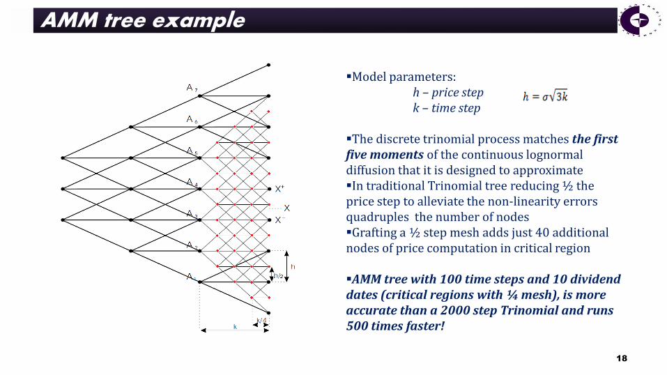
Model parameters: h – price step k – time step
The discrete trinomial process matches the first five moments of the continuous lognormal diffusion that it is designed to approximate In traditional Trinomial tree reducing ½ the price step to alleviate the non-linearity errors quadruples the number of nodes Grafting a ½ step mesh adds just 40 additional nodes of price computation in critical region
AMM tree with 100 time steps and 10 dividend dates (critical regions with ¼ mesh), is more accurate than a 2000 step Trinomial and runs 500 times faster!
4. Implementing ACCELERATED LATTICE Models in CUDA
19
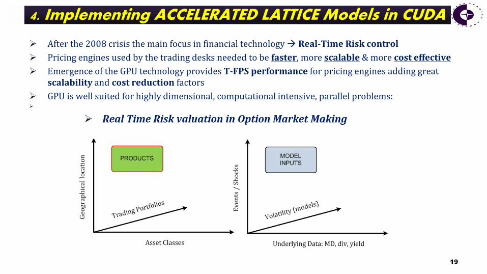
After the 2008 crisis the main focus in financial technology Real-Time Risk control
Pricing engines used by the trading desks needed to be faster, more scalable & more cost effective
Emergence of the GPU technology provides T-FPS performance for pricing engines adding great scalability and cost reduction factors
GPU is well suited for highly dimensional, computational intensive, parallel problems:
Real Time Risk valuation in Option Market Making

REAL-Time RISK Valuation in CUDA
20
GPU massive parallelization potential meets the requirements of the RT-R problem:
Millions of simultaneous calculations easily available within one process
Increased computing speed (x10-50 factors)
Dramatic reduction of the hardware footprint required to host the calculations
Better availability and scalability across products, desk and geographies
Prototyping a new generation of Pricing Engines on latest GPU devices:
2011: Quadro 4000 CUDA 2.0 256 cores / 0.95 GHz / 2 GB
2012: GTX 680 CUDA 3.0 1536 cores / 1 GHz / 6 GB
A comparison study Theo. Gain Factor
CPU : 12 core Intel Xeon X5680 / 3.57 GHz / 32 GB 1
GPU_1 : 4 x Quadro 4000 - 1024 cores / 1 GHz / 2 GB 24
GPU_2 : 2 x GTX 680/690 – 3072 cores / 1 GHz / 6 GB 72
Minimizing to the Root Mean Square error (Broadie & Detemple)
Comparative study: models & devices
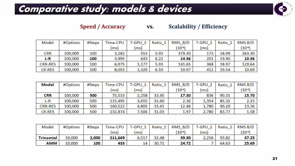
21
Speed / Accuracy vs. Scalability / Efficiency
Multiprocessor occupancy
22
The multiprocessor occupancy is the ratio of active warps to the maximum number of warps supported on a multiprocessor of the GPU:
CUDA 2.0 48 x 32 = 1536 threads / MP
CUDA 3.0 64 x 32 = 2048 threads / MP
Maximizing the occupancy can help to cover latency during global memory loads that are followed by a __syncthreads()
The occupancy is determined by the amount of shared memory and registers used by each thread block optimize the size of thread blocks in order to maximize occupancy
Higher occupancy <> higher performance. If a kernel is not bandwidth-limited or latency-limited, then increasing occupancy will not necessarily increase performance
If a kernel grid is bottlenecked by computation and not by global memory accesses, then increasing occupancy may have no effect. In fact it could create adverse effects: additional instructions, more register spills to local memory (which is off-chip), more divergent branches, etc.

Resource allocation mapping
23
Data parallelism: 1 option per block
Task parallelism: 1 tree step per thread
CUDA 3.0 • For 128 steps LR option valuation on could calculate 16 options per MP by reusing input data for same expiration (2048 threads per MP – see Occupancy XL) It takes ~ 2.5 microseconds to value (LR) an option at 128 steps 1.2 MM options / second • For 500 steps 50,000 options / second (N2 degradation)

5. FUTURE DEVELOPMENTS
24
Implementing/reusing Tri-Diagonal solvers in CUDA for Finite Differences Parallel Cyclic Reduction algorithm: a specialized version of Cyclic Reduction
designed to maintain uniform parallelism O(log2n)
“Near Real-Time” VAR calculations
Portfolio optimization via PCA and co-integration
Financial application of Topological Data Analysis A recently introduced mathematical method (using algebraic topology) to analyze
very large sets of data by capturing the shape of a point-cloud that “persists” in a dynamical setting heavy parallel problem

Bibliography
25
[1] Barone-Adesi & R.E. Whaley. “Efficient Analytic Approximation of American Options Values.”
Journal of finance, 42 (1987), pp. 301–320
[2] Cox, J. C., Ross, S. A., and Rubinstein, M. “Option Pricing: a Simplified Approach.”
Journal of Financial Economics , 7 (1979), pp. 229–264
[3] Leisen, D. P. J. “Pricing the American Put Option: a Detailed Convergence Analysis for Binomial Models.”
Journal of Economic Dynamics and Control, 22(1998), pp. 1419–1444
[4] Leisen, D., and Reimer, M. “Binomial Models for Option Valuation - Examining and Improving Convergence.”
Applied Mathematical Finance, 3(1996), pp. 319–346
[5] Broadie, M., and J.B. Detemple. “American Options Valuation: New Bounds. Approximations and a Comparison of Existing Methods.”
Review of Financial Studies, 9, No. 4 (1996), pp. 1211–1250
[6] Figlewski, S., and Gao, B. “The Adaptive Mesh Model: a New Approach to Efficient Option Pricing.” Journal of Financial Economics , 53 (1999), pp. 313–351
6. CONCLUDING REMARKS
26
GPU Technology is in use currently by Proprietary Trading firms b/c :
Deal with “high dimensionality problems”: derivatives pricing & risk and portfolio optimization GPU is the right tool for this problems
A “post-crisis” industry mandate for tighter Risk control & cost reduction
Impressive improvements orders of magnitude
Speed / Accuracy
Scalability / Efficiency
Great potential for new advances:
BIG data processing
New acceleration techniques

Q & A
27


![Merton [1976] Option Pricing When](https://cdn.vdocument.in/doc/165x107/55cf99f2550346d0339fd883/merton-1976-option-pricing-when.jpg)