
_____________________________________________________________________
CREDIT Research Paper
No. 08/09
_____________________________________________________________________
Growth and Welfare Maximization in
Models of Public Finance and
Endogenous Growth
by
Florian Misch, Norman Gemmell and Richard Kneller
Abstract
This paper evaluates the trade-off between growth and welfare maximization from
two perspectives. Firstly, it synthesizes and extends endogenous growth models with
public finance to compare the growth and welfare maximizing tax rates. Secondly, it
examines the distinct model outcomes in terms of the growth rates and welfare levels.
This comparison highlights the range of trade-offs: the growth maximizing tax rate
can lie above, below, or on the welfare maximizing equivalent. We find however that
even relatively large differences in growth and welfare maximizing tax rates translate
into relatively small differences in growth rates, and, in some cases, welfare levels.
JEL Classification: E62, H21, H50, O40
Keywords: Economic Growth, Productive Public Spending, Optimal Fiscal
Policy
_____________________________________________________________________
Centre for Research in Economic Development and International Trade,
University of Nottingham

_____________________________________________________________________
CREDIT Research Paper
No. 08/09
Growth and Welfare Maximization in
Models of Public Finance and
Endogenous Growth
by
Florian Misch, Norman Gemmell and Richard Kneller
Outline
1. Introduction
2. The Models
3. The Equilibrium in the Market Economy
4. Growth and Welfare Maximizing Policies
5. Growth and Welfare Maximizing Policies: Numerical Comparisons
6. Growth Rates and Welfare Levels under Growth and Welfare Maximization:
Numerical comparisons
7. Conclusions
The Authors Florian Misch is a PhD student at the School of Economics, University of Nottingham.
Norman Gemmell is Principal Adviser at the Treasury, New Zealand and Professorial
Research Fellow at the School of Economics, University of Nottingham. Richard
Kneller is Associate Professor in Economics at the Leverhulme Centre for Research
on Globalisation and Economic Policy, University of Nottingham.
Acknowledgements
We are grateful to Debajyoti Chakrabarty, John Creedy, Rod Falvey, seminar
participants in Melbourne and Nottingham and participants of the CSAE Conference
2008 and the 13th Australasian Macroeconomics Workshop in Sydney for helpful
discussions and comments on earlier drafts of the paper.
_____________________________________________________________________
Research Papers at www.nottingham.ac.uk/economics/credit/

1 Introduction
Comparisons between the growth maximizing and welfare maximizing �scal
policy over the long-run which have been a central issue in models of public
�nance and growth are important from a policy-making perspective: Al-
though the maximization of welfare is typically characterized as the priority
of benevolent governments, imperfect knowledge about the preferences of the
household may prevent them from pursuing a �rst-best strategy to achieve
this objective. An obvious option for a second-best strategy is growth maxi-
mization because in practice changes in welfare are more di¢ cult to measure
than income levels or growth. However, policy makers often perceive a dis-
tinction between the provision of social public services to meet objectives
related to social welfare and the policies necessary to achieve higher growth
rates.1 These issues are also important in current policy debates, especially
with respect to appropriate �scal policies for developing countries.2
This paper evaluates the conclusions regarding the trade-o¤ between
growth and welfare maximization from two perspectives. The �rst compares
the welfare maximizing and growth maximizing tax rates found in models
of public �nance and growth. In so doing we synthesize as well as extend
the theoretical literature. The key outcome of this is exercise is to highlight
the range of conclusions possible regarding the trade-o¤ between growth and
welfare maximization that can be drawn from this class of theoretical models.
The growth maximizing tax rate can be the same as, higher or lower than
the welfare maximizing equivalent, as a result of small changes in model as-
sumptions about the nature of the e¤ects of �scal policy. As is well known, in
the Barro (1990) model with a �ow of productive public services, the growth
and welfare maximizing tax rates coincide, whereas in the Futagami et al.
(1993) model with productive public capital, the growth maximizing tax rate
exceeds the welfare maximizing tax rate. In contrast, in a model with one
1For instance, the Tanzanian National Strategy for Growth and Reduction of Povertycontains a cluster for �Growth and the reduction of income poverty�and another cluster on�Improved quality of life and social well-being�that both list the provision of various publicservices and various types of public investment. The division into two clusters re�ects theperception that there are trade-o¤s.
2See for example World Bank (2007).
1
utility-enhancing, and one productive, public service derived from the �ow
of public spending, the growth maximizing tax rate lies below the welfare
maximizing rate.3
We make two further extensions to the Barro (1990) framework. In the
�rst extension we allow for the possibility that public services or public cap-
ital entail mixed e¤ects; the same public service/capital may simultaneously
be productive as well as utility-enhancing. In developing countries where the
government typically provides more rudimentary public services, it is likely
that few public services entail purely productive or purely utility-enhancing
e¤ects. For example, public transportation infrastructure may not only be
productive because it facilitates access to hospitals, and primary health facil-
ities but may also be productive because they ensure that the labour force re-
mains �t for work. Agénor and Neanidis (2006) provide a survey of empirical
evidence on the impact of health on growth and the impact of infrastructure
on health outcomes.
We also extend the model to allow for greater complementarity between
productive public services and private capital than in the Cobb-Douglas case
(the elasticity of substitution is assumed to be lower than one). Public ser-
vices provided by the government fundamentally di¤er from private inputs,
such that it may be very costly for �rms to substitute for them. For exam-
ple, poor quality road surfaces may require �rms to purchase special, more
expensive, vehicles for the transportation of goods.
We consider various combinations of these assumptions. In the �nal set
of models public services are assumed to yield productive as well as utility-
enhancing e¤ects, and the elasticity of substitution is assumed to be lower
than one. Since closed-form solutions cannot be obtained in such cases, it
is shown numerically, that with public capital that entails mixed e¤ects, the
Futagami et al. (1993) results no longer holds, and that with a higher degree
of complementarity, the same is true for the Barro (1990) result. Overall,
3Throughout the paper, the term �Barro Model�refers to the main model developed inBarro (1990), and the term �Futagami Model�refers to the model developed in Futagamiet al. (1993). The term �public services�denotes public services derived from the �ow ofpublic spending, whereas the term �public capital�is equivalent to public services derivedfrom the stock of public capital.
2

these additions serve to further decrease the generality of the conclusion
regarding the relationship between growth and welfare maximizing tax rates.
The second contribution of the paper is to provide an evaluation of the
extent to which growth and welfare maximization yield distinct outcomes
in terms of the growth rates and welfare levels along the balanced growth
path. This is a question that is often ignored in the literature, even though
di¤erences in outcomes determine the trade-o¤ between growth and welfare
maximization. This analysis is provided through numerical simulations of
policies and outcomes under growth and welfare maximization for a wide
range of parameter sets, and in particular which nest di¤erent degrees of
complementarity between public services/capital and private capital.4
The results from this exercise are striking and serve to modify the policy
conclusions that might be drawn from the �rst part of the paper. Even when
the di¤erences between the tax rate necessary to achieve growth compared
to welfare maximization are relatively large, we �nd that this translates into
relatively small di¤erences between growth rates. For models with public
services, they also translate into relatively small di¤erences in welfare levels.
That is, even where there is uncertainty about how a particular form of pub-
lic service or capital a¤ects the production function or the utility function,
in practice growth maximization yields growth outcomes (and in the case of
public services, welfare outcomes) that are very close to those found under
welfare maximization. We establish that this holds for a large array of pos-
sible parameter combinations and therefore would appear a robust result in
the developments made since the original Barro (1990) model. This �nding
suggests that with public services, growth maximization may be a suitable
second-best strategy for benevolent governments. It occurs in part because
the growth rate is a central determinant of welfare, but also because policy
is relatively ine¤ective between the welfare and the growth rate maximum.
It should be remembered, in addition, that this result occurs in a class of
models that ensure long run impacts of �scal policy, and which typically form
the reference point for any theoretical discussion of �scal policy and long-run
4We model this using a distribution function for each exogenous model parameter,allowing us to generate a large number of possible parameter sets.
3

growth.5
The remainder of the paper is organized as follows. The next section
develops the models. Section 3 derives the equilibrium in the market econ-
omy. Section 4 analytically compares the growth and welfare maximizing tax
rates. Section 5 provides some numerical comparisons of growth and welfare
maximizing tax rates, while section 6 uses numerical examples to compare
the growth rates, and welfare levels along the balanced growth path (under
both growth and welfare maximization). Finally, section 7 summarizes the
results and discusses some policy implications.
2 The Models
The public �nance growth framework we adopt in the paper is based on
Barro (1990). We assume that there is a large number of identical and
in�nitely lived households that is normalized to one, and that population
growth is zero. The household produces a single composite good which can
be used for consumption or physical capital accumulation. To incorporate
the notion of complementarity between private and public services later in
the paper the production function is a generalized version of that found in
Barro (1990). Output is produced using private capital (k) and a non-rival
and non-excludable productive public service (g):
y = (�k� + �g�)1� (1)
where � = 1� �. The parameter � determines the elasticity of substitutiongiven by:
s =1
1� � (2)
The government levies a proportional tax on output at rate � , to provide
public services. Hence:
g = �y (3)
5See Turnovsky (2004) for an excellent discussion of the long-run growth e¤ects of �scalpolicy.
4
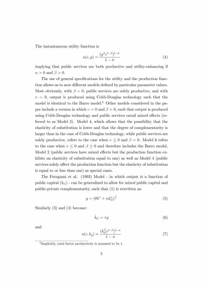
The instantaneous utility function is
u(c; g) =(g�c1��)1��
1� � (4)
implying that public services are both productive and utility-enhancing if
� > 0 and � > 0.
The use of general speci�cations for the utility and the production func-
tion allows us to nest di¤erent models de�ned by particular parameter values.
Most obviously, with � = 0, public services are solely productive, and with
� = 0, output is produced using Cobb-Douglas technology such that the
model is identical to the Barro model.6 Other models considered in the pa-
per include a version in which � = 0 and � > 0, such that output is produced
using Cobb-Douglas technology and public services entail mixed e¤ects (re-
ferred to as Model 2). Model 4, which allows that the possibility that the
elasticity of substitution is lower and that the degree of complementarity is
larger than in the case of Cobb-Douglas technology, while public services are
solely productive, refers to the case when � � 0 and � = 0. Model 6 refersto the case when � � 0 and � � 0 and therefore includes the Barro model,Model 2 (public services have mixed e¤ects but the production function ex-
hibits an elasticity of substitution equal to one) as well as Model 4 (public
services solely a¤ect the production function but the elasticity of substitution
is equal to or less than one) as special cases.
The Futagami et al. (1993) Model - in which output is a function of
public capital (kG) - can be generalized to allow for mixed public capital and
public-private complementarity, such that (1) is rewritten as:
y = (�k� + �k�G)1� (5)
Similarly (3) and (4) become:
_kG = �y (6)
and
u(c; kg) =(k�Gc
1��)1��
1� � (7)
6Implicitly, total factor productivity is assumed to be 1.
5
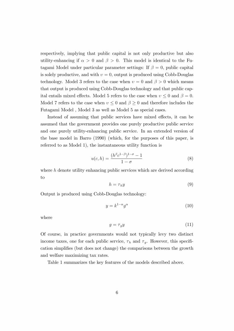
respectively, implying that public capital is not only productive but also
utility-enhancing if � > 0 and � > 0. This model is identical to the Fu-
tagami Model under particular parameter settings: If � = 0, public capital
is solely productive, and with � = 0; output is produced using Cobb-Douglas
technology. Model 3 refers to the case when � = 0 and � > 0 which means
that output is produced using Cobb-Douglas technology and that public cap-
ital entails mixed e¤ects. Model 5 refers to the case when � � 0 and � = 0.Model 7 refers to the case when � � 0 and � � 0 and therefore includes theFutagami Model , Model 3 as well as Model 5 as special cases.
Instead of assuming that public services have mixed e¤ects, it can be
assumed that the government provides one purely productive public service
and one purely utility-enhancing public service. In an extended version of
the base model in Barro (1990) (which, for the purposes of this paper, is
referred to as Model 1), the instantaneous utility function is
u(c; h) =(h�c1��)1�� � 1
1� � (8)
where h denote utility enhancing public services which are derived according
to
h = �hy (9)
Output is produced using Cobb-Douglas technology:
y = k1��g� (10)
where
g = � gy (11)
Of course, in practice governments would not typically levy two distinct
income taxes, one for each public service, �h and � g. However, this speci�-
cation simpli�es (but does not change) the comparisons between the growth
and welfare maximizing tax rates.
Table 1 summarizes the key features of the models described above.
6
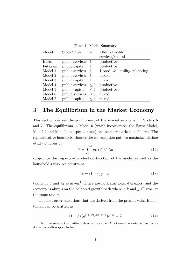
Table 1: Model Summary
Model Stock/Flow � E¤ect of publicservices/capital
Barro public services 1 productiveFutagami public capital 1 productiveModel 1 public services 1 1 prod. & 1 utility-enhancingModel 2 public services 1 mixedModel 3 public capital 1 mixedModel 4 public services � 1 productiveModel 5 public capital � 1 productiveModel 6 public services � 1 mixedModel 7 public capital � 1 mixed
3 The Equilibrium in the Market Economy
This section derives the equilibrium of the market economy in Models 6
and 7. The equilibrium in Model 6 (which incorporates the Barro Model,
Model 2 and Model 4 as special cases) can be characterized as follows. The
representative household chooses the consumption path to maximize lifetime
utility U given by
U =
Z 1
0
u(c(t))e��tdt (12)
subject to the respective production function of the model as well as the
household�s resource constraint
_k = (1� �)y � c (13)
taking � , g and k0 as given.7 There are no transitional dynamics, and the
economy is always on the balanced growth path where c, k and y all grow at
the same rate .
The �rst order conditions that are derived from the present-value Hamil-
tonian can be written as
(1� �) (g�(1��)c������)e��t = � (14)
7The time subscript is omitted whenever possible. A dot over the variable denotes itsderivative with respect to time.
7

and
(1� �)yk = �_�
�(15)
where yk is the derivative of output with respect to private capital and �
is the costate variable. In addition, the transversality condition has to be
ful�lled:
limt!1
[�k] = 0 (16)
Rearranging (14), taking logs and di¤erentiating with respect to time
yields_c
c=
1
�� � � � �_�
�+
�
�� � � � � +��(1� �)�� � � � �
_g
g(17)
Since g = �y and given that the tax rate is constant, = _gg= _y
yalong the
balanced growth path. Therefore, after setting _gg= _c
c, and after substituting
for _��using (15), (17) can be rewritten to yield
=_c
c=1
�((1� �)yk � �) (18)
Since � does not enter the latter expression, it can be noted that in the
market economy, the presence of mixed e¤ects of public services does not
a¤ect the growth rate. Disregarding the policy choice, it can be shown that
the transversality condition (16) is always ful�lled if � > 1. Therefore, for
simplicity, it will be assumed throughout the paper that � > 1 so that the
choice of � is unconstrained by the transversality condition.
For the case of the equilibrium in the market economy, Model 7 (which
incorporates the Futagami Model, and Models 3 and 5 as special cases) can
be characterized as follows. The representative household again maximizes
lifetime utility given by (12) subject to the respective production function of
the model and the household�s resource constraint (13) taking � , kG > 0 and
k0 > 0 as given.
The �rst order conditions that are derived from the present-value Hamil-
tonian can be written as
(1� �) (k�(1��)G c������)e��t = � (19)
and
(1� �)yk = �_�
�(20)
8

where yk is the derivative of output with respect to private capital and �
is the costate variable. In addition, the transversality condition has to be
ful�lled.
Rearranging (19), taking logs and di¤erentiating with respect to time,
then yields:
_c
c=
1
�� � � � �_�
�+
�
�� � � � � ��(1� �)�� � � � �
_kGkG
(21)
The growth rate of public capital is
_kGkG=�y
kG(22)
Substituting _��and
_kGkGin (21) using (20) and (22) yields the growth rate
of consumption:_c
c=((1� �)yk � �+ �(1� �) �ykG )
� + � � �� (23)
Along the balanced growth path, = _cc=
_kk=
_kGkGso that (23) can be
rewritten as
=_c
c=1
�((1� �)yk � �) (24)
The Appendix shows that the equilibrium of the models is saddlepoint stable
within the relevant parameter ranges, and that the balanced growth path is
unique.8
In Model 1, where productive and utility-enhancing public services are
separate, utility maximization is subject to the households� resource con-
straint now given by:_k = (1� �h � � g)y � c (25)
The households take � g, �h, g, h and k0 as given. There are no transitional
dynamics, and the economy is always on the balanced growth path. It can
be shown that the growth rate of the economy can be expressed as
=_c
c=1
�((1� �h � � g)yk � �) (26)
which is equivalent to (24) where �h + � g = � .
8It is again assumed that � > 1 so that the transversality condition is ful�lled.
9
4 Growth and Welfare Maximizing Policies
4.1 The Base Models
This section derives the growth maximizing tax rate, � �, and the welfare
maximizing tax rate, � ��, in the Barro Model , in the Futagami Model, and
in Model 1. Inserting (A.5) in (18), the growth rate in the Barro Model can
be expressed as
=1
�
�(1� �)(1� �)�
�1�� � �
�(27)
Maximizing the latter expression for � yields the familiar growth maximizing
tax rate for the Barro Model , � �B, as:
� �B = � (28)
Output net of taxation can be written as
y = (1� �)��
1��k
It can easily be seen that maximizing output net of taxation at every point
of time yields the same tax rate as maximizing the growth rate. Therefore,
in the Barro Model, there are no trade-o¤s between growth maximization
and welfare maximization, and the growth and the welfare maximizing tax
rate coincide:
� �B = ���B = � (29)
Inserting (A.16) in (24), the growth rate in the Futagami Model can be
expressed as
=1
�
�(1� �) (1� �) (�
)
�1�� � �
�(30)
Using implicit di¤erentiation, it can be shown that the growth maximizing
tax rate is
� �F = � (31)
Under welfare maximization in the market economy, the government maxi-
mizes (12) subject to (13) and (6) while taking the �rst order conditions of
10
the households as given. Futagami et al. (1993) have shown that the growth
maximizing tax rate exceeds the welfare maximizing one:
� �F = � > ���F (32)
The reason is that when public services are derived from the stock of public
capital, consumption is foregone in the process of accumulating public capital
(Turnovsky (1997)) so that maximizing output and maximizing the growth
rates are no longer identical. This e¤ect is termed the �capital accumulation
e¤ect�.
Turnovsky (1997) derives an expression for the welfare maximizing tax
rate of a centrally planned economy and considers relative congestion. For
the market economy, no closed-form solution for the welfare maximizing tax
rate can be found. Along the lines of Ghosh and Roy (2004), it is shown
in the Appendix that the welfare maximizing tax rate, � ��F , has to satisfy
equations (A.44) and (A.46) when � = 0 (which are both restated here for
convenience):
ykG = (1� �)yk (33)
�y
kG=1
�((1� �)yk � �) (34)
Expressions for yk, ykG, yk and ykG are derived in the Appendix .
The growth rate in Model 1 is similar to the one in the Barro Model (27):
=1
�
�(1� �h � � g)(1� �)�
�1��g � �
�(35)
It is obvious that under growth maximization, �h is zero9 because �h has
an unambiguously negative e¤ect on the growth rate. In contrast to this,
under welfare maximization, �h is positive if � > 0. This e¤ect is termed the
�utility-enhancement e¤ect�.
Following an extension of his base model, by Barro (1990), there are
several papers that assume a utility function of the form u = u(c; h) and
9�h = 0 only holds under growth maximization if one ignores the fact that with nospending on h, households do not derive any utility from economic activity. Therefore, amore realistic assumption would be that under growth maximization, �h still has to bepositive.
11
compare the growth and welfare maximizing tax rate, including Lau (1995),
Park and Philippopoulous (2002), as well as Greiner and Hanusch (1998). Of
such models, Model 1 probably captures the distinction between growth and
welfare maximization with utility-enhancing public services that is typically
perceived among policy makers. In this model, the welfare maximizing level
of taxation clearly exceeds the growth maximizing level, and maximizing
welfare unambiguously lowers the growth rate.
The next subsection extends the above models to allow for �mixed�public
services and complementarity between public and private capital.
4.2 The Extended Models
This sub-section �rst analytically derives the growth and welfare maximiz-
ing tax rates in models with public services that incorporate mixed e¤ects,
complementarity, or both (Models 2, 4 and 6), and then considers the equiv-
alent results in models with public capital (Models 3, 5 and 7). To simplify
the exposition, in Models 4 to 7, the elasticity of substitution is assumed to
be 12(implying � = �1), which is halfway between the Cobb-Douglas and
Leontief technologies. This yields a larger (smaller) degree of complementar-
ity between the inputs to private production than Cobb-Douglas (Leontief)
technology.
In Model 2, the growth maximizing tax rate, � �2, corresponds to the Barro
Model since the production functions are identical. Hence:
� �2 = � (36)
In Models 4 and 6, using (A.9) and (A.8) to substitute for yk in (18), and
with � = �1, the growth rate can be written as
=1
�
�(1� �)(� + ��
(� � �))�2� � �
�(37)
Maximizing the latter expression yields the growth maximizing tax rates, � �4and � �6:
� �4 = ��6 =
1
2(p�2 + 8�� �) (38)
12
Since there are no transitional dynamics in Models 2, 4 and 6, the welfare
maximizing tax rate can be derived as follows. With x = ck, lifetime utility
can be written as
U =
Z 1
0
��gk
��x1��k(t)
�1��1� � e��tdt (39)
Along the balanced growth path, x and gkare constant, and _k
k= , such that:
k = k0e t (40)
Therefore, along the balanced growth path, (39) can be expressed as (ignoring
the constants):
U =1
1� �
264��
gk
��x1��
�1���� (1� �)
375 (41)
Maximizing the latter expression (after substituting for x = _cc� (1 � �) y
k
and for gkusing (A.8), and setting � = 0 for Model 4) yields the welfare
maximizing tax rate of Model 2 (� ��2 ), Model 4 (���4 ) and Model 6 (�
��6 ).
Closed-form solutions cannot be obtained.
In Model 3, the growth maximizing tax rate corresponds to the Futagami
Model since the production functions are identical, hence:
� �3 = � (42)
In Model 5 and 7, the growth maximizing tax rate can be found by maximiz-
ing (24) using implicit di¤erentiation in a similar way to the Futagami Model.
However, no closed-form solution exists. Similarly, there are no closed-form
solutions available for the welfare maximizing tax rate in Model 3, 5 and 7.10
We therefore rely on numerical simulations, discussed in sections 5 and 6.
There are only few models in the existing literature that consider mixed
public services and mixed public capital that are both utility-enhancing and
10As shown in the Appendix, the welfare-maximizing tax rate has to satisfy equations(A.44), (A.46) and (A.47). Expressions for y
k ,ykG, yk and ykG which di¤er between the
models are derived in the Appendix.
13

productive.11 In part due to their complexity, the growth maximizing and
the welfare maximizing income tax rates are generally not compared for the
decentralized economy. The most straightforward version can be found in
Balldicci (2005), who develops a Barro-style model in which the government
provides mixed public services derived from the �ow of public spending. He
�nds that within a centrally planned economy, the welfare maximizing tax
rate exceeds the growth maximizing one.
A more complicated approach is adopted in a series of papers by Agénor.
Agénor and Neanidis (2006) introduce a model in which �nal output is pro-
duced using private capital, public services derived from spending on in-
frastructure and e¤ective labour which in turn depends on health services
and on the share of educated workers in production. Educated labour is
produced using, among other inputs, raw labour, health services and public
spending on education. Health services in turn are produced using educated
labour, public spending on health and spending on infrastructure, and in
addition to being productive are also utility-enhancing.
Agénor and Neanidis (2006) compare the growth maximizing allocation
of government revenue in a decentralized economy to the welfare maximizing
allocation of government revenue in a centrally planned economy treating
the tax rate and the share of one category of public spending as exogenously
set. They examine trade-o¤s between the three spending shares: infrastruc-
ture, education and health. They �nd that the welfare maximizing shares
of infrastructure spending, and of education spending, in total revenue when
o¤set by spending on health are lower than the growth maximizing shares
(in the �rst case, the share of spending on education and in the second case,
the share of spending on infrastructure is exogenously set). This implies that
the welfare maximizing share of health spending is higher than the growth
maximizing equivalent.
Agénor (2005) presents a model with health and infrastructure public
services. The former are both productive and utility-enhancing. In the �rst
11Comparing welfare maximizing and growth maximizing �scal policies within a modelin which public capital is productive and utility-reducing due to negative welfare e¤ectsof growth (pollution) is proposed for further research by Greiner and Kuhn (2003).
14

version of the model, both types of public services are derived from the
�ow of public spending on health and infrastructure. He shows that in a
centrally planned economy, the welfare maximizing tax rate and the welfare
maximizing share of health spending in total government revenue exceed the
corresponding growth maximizing equivalents in a decentralized economy. In
the second version of the model, health services are derived from the stock
of health capital that is accumulated using public spending on health and
spending on infrastructure. In this case the stock of health capital entails
mixed e¤ects. However, welfare maximizing policies are not derived for this
version of the model.
Likewise, there are a few papers that consider CES technology within
endogenous growth models with public spending. Even here, growth and
welfare maximizing policies are typically not compared for a decentralized
economy. Devarajan et al. (1996) introduce a model in which output is
produced using private capital and two productive public services with CES
technology, but they do not study optimal policies. Baier and Glomm (2001)
alternatively consider a case in which output is produced using labour, private
capital and public capital and allow for varying degrees of substitutability
between public and private capital. They show numerically that the growth
maximizing size of the public sector increases as the elasticity of substitution
decreases. Finally, Ott and Turnovsky (2006) introduce a model in which
the government provides a non-excludable and an excludable public service
that are both subject to congestion �nanced by income taxes and user fees.
They �nd that for the centrally planned economy with CES technology, the
growth and welfare maximizing expenditure shares in output (which essen-
tially correspond to the tax rates) coincide. Ott and Turnovsky (2006) also
derive welfare maximizing �scal policies for the decentralized economy.
5 Growth and Welfare Maximizing IncomeTax Rates: Numerical Comparisons
Due to the lack of closed-form solutions in several versions of the model, in
this section we present numerical comparisons between growth and welfare
15

maximization. Speci�cally, we plot the growth and welfare maximizing tax
rates as functions of � in the alternative models. This allows us to compare
the growth and welfare maximizing tax rates across a wide range of parame-
ter con�gurations, and provides an indication of the magnitude of potential
di¤erences. Again, for simplicity, the elasticity of substitution in models 4
to 7 is assumed to be 12(implying � = �1).
Figure 1 plots the welfare and growth maximizing tax rates in the Fu-
tagami Model, Model 2 and Model 3. The growth and welfare maximizing
tax rates of the Barro Model are also implicitly considered since they corre-
spond to the growth maximizing tax rate that coincides across these models.
As shown in the previous section, due to the capital accumulation e¤ect,
the welfare maximizing tax rate in the Futagami Model is lower than the
growth maximizing one. In contrast to this, the welfare maximizing tax rate
in the model with mixed public services (Model 2) exceeds the growth max-
imizing tax rate. That is, due to the simultaneous utility-enhancing e¤ect
of public services, higher levels are desirable from a welfare perspective. As
might be expected from this con�guration of results when we consider the
model with mixed public capital (Model 3), the impact of increasing � on
the relative position of the welfare maximizing tax rate is ambiguous. The
utility-enhancement e¤ect and the capital accumulation e¤ect oppose each
other. For low values of � the welfare maximizing tax rate is below the
growth maximizing rate, whereas for high values of � it lies above it, and
16

there exist a particular value of � when both tax rates are identical.
Figure 1: The tax rate as a function of �
In Figure 2 we plot the welfare and growth maximizing tax rates for
Models 4 and 6. In Model 4 - the model with public services but an elasticity
of substitution less than one - the welfare maximizing tax rate is not a¤ected
by �. However, it no longer matches the growth maximizing tax rate, and
the welfare maximizing tax rate is always lower. As Barro (1990) predicts,
the elasticity of substitution a¤ects the relationship between the welfare and
growth maximizing tax rates. The reason is that maximizing output net of
taxation is no longer identical to maximizing the growth rate. When we allow
for mixed public services in the model with an elasticity of substitution less
than one (Model 6), we �nd that the welfare maximizing tax rate increases
with �, and its position with regard to the growth maximizing tax rate is
ambiguous. A smaller elasticity of substitution lowers the welfare maximizing
tax rate, whereas the utility-enhancement e¤ect (which increases with �)
raises it. For low values of � the welfare maximizing tax rate is below the
17
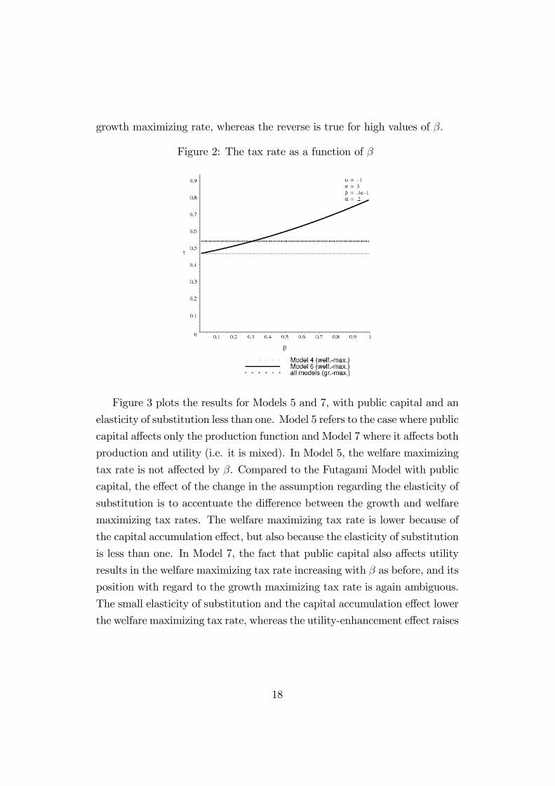
growth maximizing rate, whereas the reverse is true for high values of �.
Figure 2: The tax rate as a function of �
Figure 3 plots the results for Models 5 and 7, with public capital and an
elasticity of substitution less than one. Model 5 refers to the case where public
capital a¤ects only the production function and Model 7 where it a¤ects both
production and utility (i.e. it is mixed). In Model 5, the welfare maximizing
tax rate is not a¤ected by �. Compared to the Futagami Model with public
capital, the e¤ect of the change in the assumption regarding the elasticity of
substitution is to accentuate the di¤erence between the growth and welfare
maximizing tax rates. The welfare maximizing tax rate is lower because of
the capital accumulation e¤ect, but also because the elasticity of substitution
is less than one. In Model 7, the fact that public capital also a¤ects utility
results in the welfare maximizing tax rate increasing with � as before, and its
position with regard to the growth maximizing tax rate is again ambiguous.
The small elasticity of substitution and the capital accumulation e¤ect lower
the welfare maximizing tax rate, whereas the utility-enhancement e¤ect raises
18
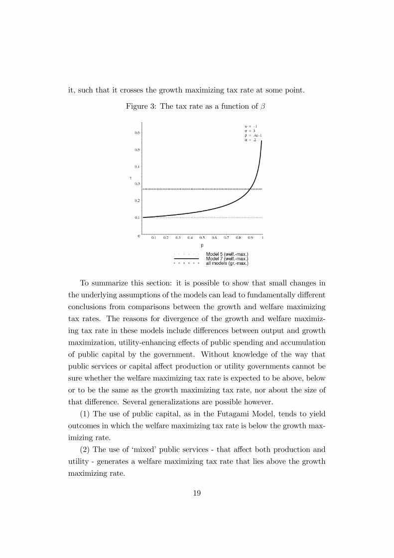
it, such that it crosses the growth maximizing tax rate at some point.
Figure 3: The tax rate as a function of �
To summarize this section: it is possible to show that small changes in
the underlying assumptions of the models can lead to fundamentally di¤erent
conclusions from comparisons between the growth and welfare maximizing
tax rates. The reasons for divergence of the growth and welfare maximiz-
ing tax rate in these models include di¤erences between output and growth
maximization, utility-enhancing e¤ects of public spending and accumulation
of public capital by the government. Without knowledge of the way that
public services or capital a¤ect production or utility governments cannot be
sure whether the welfare maximizing tax rate is expected to be above, below
or to be the same as the growth maximizing tax rate, nor about the size of
that di¤erence. Several generalizations are possible however.
(1) The use of public capital, as in the Futagami Model, tends to yield
outcomes in which the welfare maximizing tax rate is below the growth max-
imizing rate.
(2) The use of �mixed�public services - that a¤ect both production and
utility - generates a welfare maximizing tax rate that lies above the growth
maximizing rate.
19
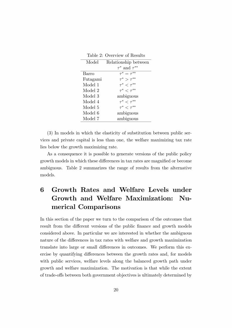
Table 2: Overview of Results
Model Relationship between� � and � ��
Barro � � = � ��
Futagami � � > � ��
Model 1 � � < � ��
Model 2 � � < � ��
Model 3 ambiguousModel 4 � � < � ��
Model 5 � � < � ��
Model 6 ambiguousModel 7 ambiguous
(3) In models in which the elasticity of substitution between public ser-
vices and private capital is less than one, the welfare maximizing tax rate
lies below the growth maximizing rate.
As a consequence it is possible to generate versions of the public policy
growth models in which these di¤erences in tax rates are magni�ed or become
ambiguous. Table 2 summarizes the range of results from the alternative
models.
6 Growth Rates and Welfare Levels underGrowth and Welfare Maximization: Nu-merical Comparisons
In this section of the paper we turn to the comparison of the outcomes that
result from the di¤erent versions of the public �nance and growth models
considered above. In particular we are interested in whether the ambiguous
nature of the di¤erences in tax rates with welfare and growth maximization
translate into large or small di¤erences in outcomes. We perform this ex-
ercise by quantifying di¤erences between the growth rates and, for models
with public services, welfare levels along the balanced growth path under
growth and welfare maximization. The motivation is that while the extent
of trade-o¤s between both government objectives is ultimately determined by
20
di¤erences in outcomes, most papers solely focus on di¤erences in policies.
An exception is Monteiro and Turnovsky (2007) who develop a two-sector
endogenous growth model with physical and human capital. The government
provides one public service that enhances the production of �nal output and
one public service that enhances the production of human capital. Both
are derived from the �ow of public expenditure. They present steady state
growth rates and steady state welfare levels for several di¤erent combinations
of the tax rate and public spending composition (under two alternative set-
tings of the remaining model parameters). Whereas utility is derived from
consumption, which in turn is derived from �nal output, the welfare bene-
�ts of spending on the production of human capital are less direct. They
therefore �nd a trade-o¤ between growth and welfare maximization.
The previous section has shown that it is di¢ cult to draw speci�c con-
clusions from comparisons between the growth and welfare maximizing tax
rates. As a result trade-o¤s in terms of �scal policies are very di¢ cult to
predict if the precise model speci�cation, and the speci�c values of key para-
meters, are unknown. To deal with this model and parameter uncertainty we
numerically evaluate the growth rates and welfare levels along the balanced
growth path for a large number of di¤erent values of the exogenous model
parameters. By doing so it is hoped that general conclusions about growth
and welfare maximization can be derived even under model and parameter
uncertainty.
The procedure used consists of two steps:12 First, a large number of val-
ues for each exogenous model parameter were generated. No assumptions
regarding the speci�c parameter values were made. Rather, each parameter
is allowed to vary across some (plausible) range. The lower bound (l) and
the upper bound (u) are chosen to re�ect theoretical restrictions, economet-
ric estimates and/or anecdotal evidence where available. Two alternative
distributions are assumed between the lower and upper bound. First, a Uni-
form distribution, and second, a symmetric Normal distribution (with mean,
� = (l+u)2, and standard deviation, s = (u�l)
1:96) are used. 7728 parameter sets
were then generated based on 7728 independent draws for each distribution.
12We use the same method as Salhofer et al. (2001) who apply it in a di¤erent context.
21

Table 3: Exogenous Parameter Ranges and Distribution
s u Distribution 1 Distribution 2� 1:001 3 Uniform Normal� 0:02 0:06 Uniform Normal� 0:1 0:45 Uniform Normal� 0 0:6 Uniform Normal� �1 �0:001 Uniform Normal
Table 4: Normal Parameter Distribution
Mean Std. Dev. Min. Max.� 2.002 0.443 1.001 2.999� 0.04 0.009 0.02 0.06� 0.273 0.078 0.1 0.45� 0.299 0.134 0 0.6� -0.499 0.224 -1 -0.001N 7728
Each parameter set includes values for all exogenous parameters in Models
6 and 7. Table 3 summarizes the parameter assumptions; Tables 4 and 5
summarize the simulated distributions resulting from the 7728 independent
draws.
Secondly, the maximization procedures, and the resulting outcomes in
both models, were solved numerically for the Uniformly and Normally dis-
tributed parameter values. The growth and welfare maximizing tax rates, � �
and � �� were calculated in the same way as in Models 6 and 7 (where � takes
the values within the range de�ned above). To compare both tax rates, the
Table 5: Uniform Parameter Distribution
Mean Std. Dev. Min. Max.� 2.002 0.581 1.001 2.999� 0.04 0.012 0.02 0.06� 0.273 0.101 0.1 0.45� 0.296 0.173 0 0.6� -0.501 0.287 -1 -0.001N 7728
22

relative di¤erence is calculated as:����(� �� � � �)� �
����� 100 (43)
We then compare the growth rates and welfare levels that result from these
di¤erent growth and welfare maximizing �scal policies. For Model 6, growth
rates and welfare levels along the balanced growth path under growth and
welfare maximization, � and �� as well W � and W ��, are calculated. The
level of welfare along the balanced growth path is calculated based on (41).
To compare growth rates and welfare under both objectives, it is again useful
to calculate relative di¤erences, given by
( � � ��) �
� 100 (44)
and(W �� �W �)
W �� � 100 (45)
respectively. In Model 7, due to transitional dynamics, (41) is not identical
to lifetime utility. That is, while the welfare maximizing tax rate yields the
highest possible lifetime utility, it does not necessarily represent the high-
est welfare levels along the balanced growth path. Since no expression for
lifetime utility is available for models with public capital, the comparison
between welfare under growth and welfare maximization in these models is
not feasible.
Summary statistics for Model 6 are shown in Tables 6 and 7. The tables
show that, for both distributions, the mean and standard deviation of the
relative di¤erence between the growth and welfare maximizing tax rates are
much larger than for the relative di¤erence between the growth rate and
welfare under growth and welfare maximization. The mean di¤erence in tax
rates is calculated at 14%, while the mean di¤erence in growth rates that
result from these is less than 2.4% and the mean of the relative di¤erence
of welfare levels is less than 4.3%. For the Normal distribution, di¤erences
are smaller than for the Uniform distribution, re�ecting the fact that under
the Normal distribution the probability of extreme values is smaller. The
standard deviations (of relative di¤erences) are also large in absolute terms
23
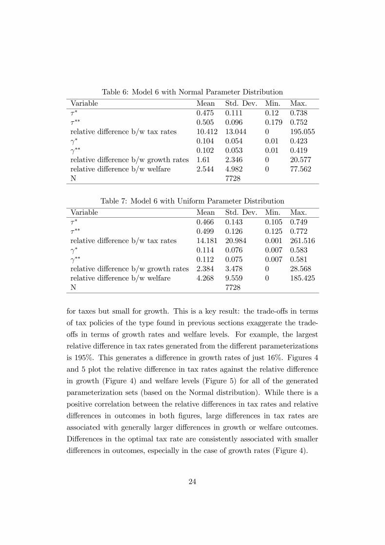
Table 6: Model 6 with Normal Parameter Distribution
Variable Mean Std. Dev. Min. Max.� � 0.475 0.111 0.12 0.738� �� 0.505 0.096 0.179 0.752relative di¤erence b/w tax rates 10.412 13.044 0 195.055 � 0.104 0.054 0.01 0.423 �� 0.102 0.053 0.01 0.419relative di¤erence b/w growth rates 1.61 2.346 0 20.577relative di¤erence b/w welfare 2.544 4.982 0 77.562N 7728
Table 7: Model 6 with Uniform Parameter Distribution
Variable Mean Std. Dev. Min. Max.� � 0.466 0.143 0.105 0.749� �� 0.499 0.126 0.125 0.772relative di¤erence b/w tax rates 14.181 20.984 0.001 261.516 � 0.114 0.076 0.007 0.583 �� 0.112 0.075 0.007 0.581relative di¤erence b/w growth rates 2.384 3.478 0 28.568relative di¤erence b/w welfare 4.268 9.559 0 185.425N 7728
for taxes but small for growth. This is a key result: the trade-o¤s in terms
of tax policies of the type found in previous sections exaggerate the trade-
o¤s in terms of growth rates and welfare levels. For example, the largest
relative di¤erence in tax rates generated from the di¤erent parameterizations
is 195%. This generates a di¤erence in growth rates of just 16%. Figures 4
and 5 plot the relative di¤erence in tax rates against the relative di¤erence
in growth (Figure 4) and welfare levels (Figure 5) for all of the generated
parameterization sets (based on the Normal distribution). While there is a
positive correlation between the relative di¤erences in tax rates and relative
di¤erences in outcomes in both �gures, large di¤erences in tax rates are
associated with generally larger di¤erences in growth or welfare outcomes.
Di¤erences in the optimal tax rate are consistently associated with smaller
di¤erences in outcomes, especially in the case of growth rates (Figure 4).
24
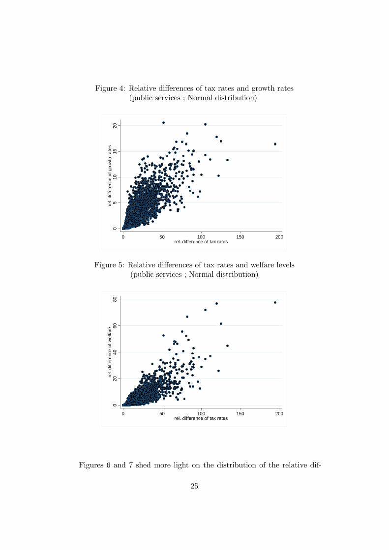
Figure 4: Relative di¤erences of tax rates and growth rates(public services ; Normal distribution)
05
1015
20re
l. di
ffere
nce
of g
row
th ra
tes
0 50 100 150 200rel. difference of tax rates
Figure 5: Relative di¤erences of tax rates and welfare levels(public services ; Normal distribution)
020
4060
80re
l. di
ffere
nce
of w
elfa
re
0 50 100 150 200rel. difference of tax rates
Figures 6 and 7 shed more light on the distribution of the relative dif-
25
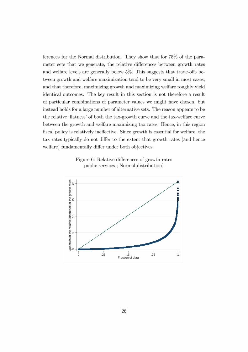
ferences for the Normal distribution. They show that for 75% of the para-
meter sets that we generate, the relative di¤erences between growth rates
and welfare levels are generally below 5%. This suggests that trade-o¤s be-
tween growth and welfare maximization tend to be very small in most cases,
and that therefore, maximizing growth and maximizing welfare roughly yield
identical outcomes. The key result in this section is not therefore a result
of particular combinations of parameter values we might have chosen, but
instead holds for a large number of alternative sets. The reason appears to be
the relative ��atness�of both the tax-growth curve and the tax-welfare curve
between the growth and welfare maximizing tax rates. Hence, in this region
�scal policy is relatively ine¤ective. Since growth is essential for welfare, the
tax rates typically do not di¤er to the extent that growth rates (and hence
welfare) fundamentally di¤er under both objectives.
Figure 6: Relative di¤erences of growth ratespublic services ; Normal distribution)
05
1015
20Q
uant
iles
of th
e re
lativ
e di
ffere
nce
of th
e gr
owth
rate
s
0 .25 .5 .75 1Fraction of data
26
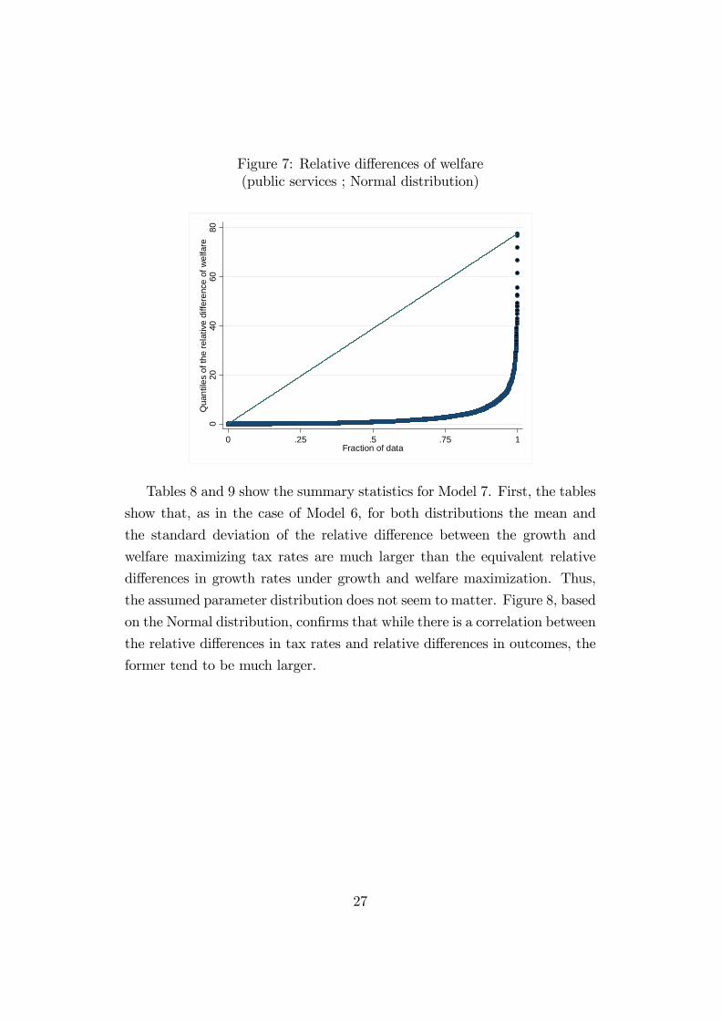
Figure 7: Relative di¤erences of welfare(public services ; Normal distribution)
020
4060
80Q
uant
iles
of th
e re
lativ
e di
ffere
nce
of w
elfa
re
0 .25 .5 .75 1Fraction of data
Tables 8 and 9 show the summary statistics for Model 7. First, the tables
show that, as in the case of Model 6, for both distributions the mean and
the standard deviation of the relative di¤erence between the growth and
welfare maximizing tax rates are much larger than the equivalent relative
di¤erences in growth rates under growth and welfare maximization. Thus,
the assumed parameter distribution does not seem to matter. Figure 8, based
on the Normal distribution, con�rms that while there is a correlation between
the relative di¤erences in tax rates and relative di¤erences in outcomes, the
former tend to be much larger.
27
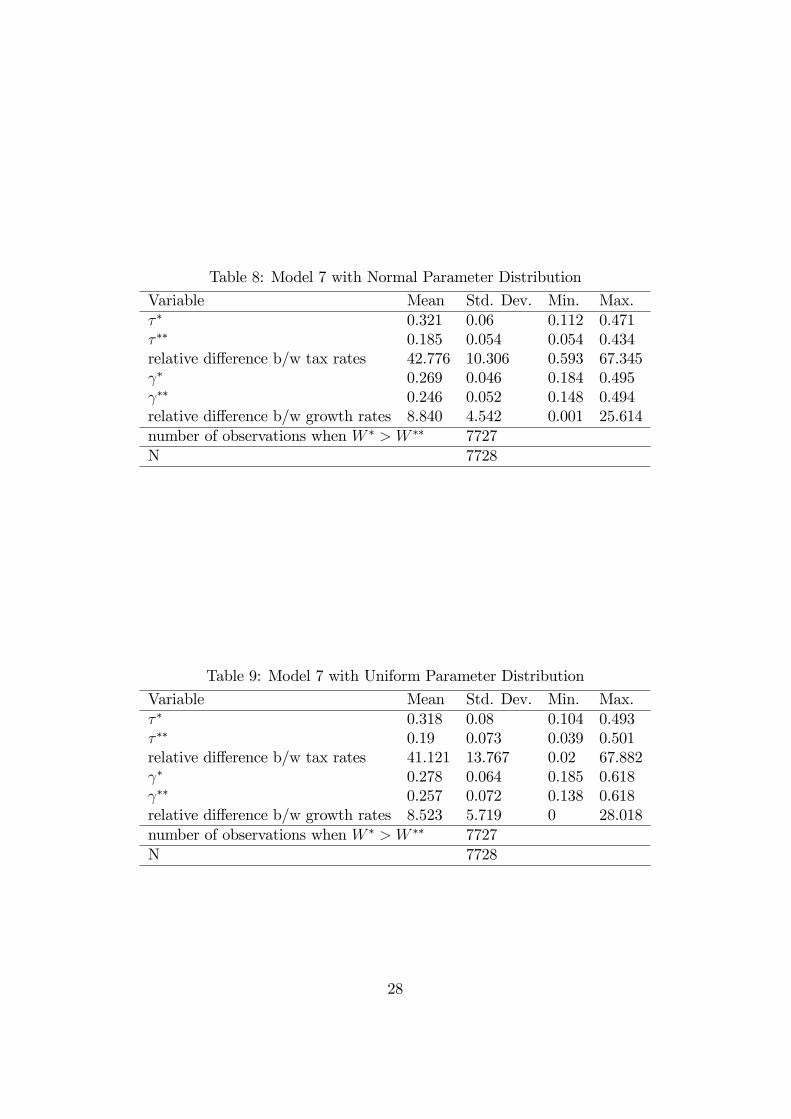
Table 8: Model 7 with Normal Parameter Distribution
Variable Mean Std. Dev. Min. Max.� � 0.321 0.06 0.112 0.471� �� 0.185 0.054 0.054 0.434relative di¤erence b/w tax rates 42.776 10.306 0.593 67.345 � 0.269 0.046 0.184 0.495 �� 0.246 0.052 0.148 0.494relative di¤erence b/w growth rates 8.840 4.542 0.001 25.614number of observations when W � > W �� 7727N 7728
Table 9: Model 7 with Uniform Parameter Distribution
Variable Mean Std. Dev. Min. Max.� � 0.318 0.08 0.104 0.493� �� 0.19 0.073 0.039 0.501relative di¤erence b/w tax rates 41.121 13.767 0.02 67.882 � 0.278 0.064 0.185 0.618 �� 0.257 0.072 0.138 0.618relative di¤erence b/w growth rates 8.523 5.719 0 28.018number of observations when W � > W �� 7727N 7728
28

Figure 8: Relative di¤erences of tax rates and growth rates(public services ; Normal distribution)
05
1015
2025
rel.
diffe
renc
e of
gro
wth
rate
s
0 20 40 60 80rel. difference of tax rates
Secondly, Tables 8 and 9 also show that the mean relative di¤erence in
growth rates between growth and welfare maximization is below 9%. Com-
pared to the model with public services, this is noticeably larger. The reason
is that with public capital there are transitional dynamics, with total welfare
driven to a lesser extent by the growth rate along the balanced growth path.
Therefore, growth and welfare maximizing tax rates, and hence growth rates,
di¤er much more with public capital. Figure 9 sheds more light on the dis-
tribution of the relative di¤erences for the Normal distribution case. They
show that for 75% of the parameter sets, the relative di¤erence between
growth rates is less than 12.5% (e.g. 3% compared with 3.375%). This sug-
gests that growth rate trade-o¤s between growth and welfare maximization
tend to be moderate in most cases. Given that no expression for lifetime
utility is available when transitional dynamics occur, trade-o¤s in terms of
welfare cannot be analyzed. However, as shown in Tables 7 and 8, along the
balanced growth path welfare is typically larger under growth maximization
than under welfare maximization because the welfare maximizing policy re-
�ects transitional dynamics. This implies that along the balanced growth
path, the welfare maximizing policy in Model 7 may not be optimal.
29

Figure 9: Relative di¤erences of tax rates and growth rates(public services ; Normal distribution)
05
1015
2025
Qua
ntile
s of
the
rela
tive
diffe
renc
e of
the
grow
th ra
tes
0 .25 .5 .75 1Fraction of data
7 Conclusions
This paper has considered the di¤erence between growth and welfare max-
imization by comparing income tax rates under both maximizations in dif-
ferent versions of a model of endogenous growth with �scal policy. It has
also compared growth rates and welfare levels as outcomes of �scal policy in
these di¤erent models. Several conclusions can be drawn from this exercise.
Firstly, comparisons between the growth and welfare maximizing tax rates
across several di¤erent models show that the central results of the existing
literature are not robust to small changes in their underlying assumptions.
The results depend crucially on the way that �scal policy is assumed to be
e¤ective. The Barro (1990) result does not hold if public services entail mixed
e¤ects, or if it is assumed that the elasticity of substitution is less than one.
The Futagami et al. (1993) result no longer holds if public capital entails
mixed public services. Likewise, it was shown that even if public services
enter the utility function, the relationship between the growth and welfare
30
maximizing tax rates is ambiguous, and the two may even coincide. These
comparisons show that for this class of endogenous growth models, without
exact knowledge of the model parameters, di¤erences between the growth
and welfare maximizing �scal policies are hard to predict.
The second conclusion modi�es the policy concerns raised by the �rst.
The relative di¤erences between growth and welfare maximizing tax rates
tend to be much larger than relative di¤erences between growth rates for
models with public services and public capital, and welfare levels for models
with public services. It was shown that relative welfare and growth trade-o¤s
in models with public services are very small, while in models with public
capital, the growth trade-o¤ is larger but still seems moderate. Parameter
uncertainty was handled by assuming a distribution function of all parame-
ters instead of adopting speci�c values. Conditional on the general class of
models, this would appear to imply that the choice between growth and wel-
fare maximization is unlikely to have large impacts on growth and, in the
case of models with public services, on welfare levels.
While this might motivate investigations of whether the same conclusions
hold in a di¤erent class of growth models, it should be remembered that the
Barro Model and its extensions form a key reference point in policy dis-
cussions of the long-run growth e¤ects of �scal policy. Possible extensions
include adding additional factors that cause the welfare maximizing tax rate
to diverge from the growth maximizing rate, such as adjustment costs and
public good congestion previously identi�ed in the literature. Alternatively
the framework might be usefully extended to allow for several sources of
public revenue or, in the spirit of Devarajan et al. (1996), several public
services. Future research would therefore ideally compare growth and wel-
fare maximization for several di¤erent instruments of �scal policy in models
that contain several sources for divergence between the growth and welfare
maximizing tax rates.
The results of this paper, though derived from relatively abstract models,
have important policy implications. The knowledge available to governments
is inevitably imperfect: they typically face informational constraints with re-
gard to household preferences and the magnitude of the utility-enhancing
31
e¤ects of public services. The results of this paper suggest that the welfare
trade-o¤s between growth and welfare maximization may be small; we �nd
many cases where the growth maximizing �scal policy yields roughly the
same welfare outcome as the welfare maximizing policy. If growth rates are
indeed susceptible to �scal policy, and if the growth enhancing e¤ect of public
services are easier to measure, then benevolent governments might reason-
ably seek to maximize the growth rate instead as a second-best strategy. In
addition, the results show that �scal policy tends to be relatively ine¤ective
in altering welfare levels and growth rates between the growth and welfare
maximizing tax rates, at least in models with public services. Changes in
�scal policy within this interval can be expected to have only a small impact
on the economy.
32

A Appendix
A.1 Expressions for y, yk and ykG
In the Barro Model and in Model 2, the production function is
y = g�k1�� (A.1)
Since
g = �y (A.2)
(A.1) can be rearranged so that
y
k= �
�1�� (A.3)
Using (A.2) and (A.3) yields an expression for gk:
g
k= �
11�� (A.4)
Di¤erentiating (A.1) for k and using (A.4) for substitute for gkyields
yk = (1� �)��
1�� (A.5)
In Models 4 and 6, the production function is
y = (�k� + �g�)1� (A.6)
Using (A.2) to substitute for g in (A.6) and rearranging yields
y
k= �
1� (1� ���)�
1� (A.7)
Using (A.2) and (A.7) yields an expression for gk:
g
k= ��
1� (1� ���)�
1� (A.8)
Di¤erentiating (A.1) for k yields
yk = (� + ��gk
��)1��1� (A.9)
with gkde�ned according to (A.8).
33

In the Futagami Model and in Model 3, the production function is
y = k�Gk1�� (A.10)
Since along the balanced growth path, private capital, public capital, con-
sumption and output all grow at the same rate given by (24),
y =_y
(A.11)
Using the (A.11) to substitute for y in _kg = �y yields
_kg = �_y
(A.12)
Integrating and rearranging yields
kg = �y
(A.13)
Substituting for kg in (A.10) and rearranging yields
y
k=
��
� �1��
(A.14)
Using (A.14) and (A.12), z = kGkcan be written as
z = (�
)
11�� (A.15)
Di¤erentiating (A.10) for k and using (A.15) to substitute for z yields
yk = (1� �)�
�1��
(A.16)
In Models 5 and 7, the production function is
y = (�k� + �k�G)1� (A.17)
Manipulations yield expressions for ykand for y
kG
y
k= (� + �z�)
1� (A.18)
y
kG= (�z�� + �)
1� (A.19)
34

Di¤erentiating (A.17) for k yields
yk = (� + �z�)
1��1� (A.20)
Di¤erentiating (A.17) for kG yields
ykG = (�z�� + �)
1��1� (A.21)
An expression for z can be found in the same way as above.
A.2 Uniqueness and Stability in Model 7
Let x = ckand z = kG
k. Together with the transversality condition, lim
t!1[�k] =
0, and with the initial conditions, x0 > 0 and z0 > 0, the dynamics of the
market economy can be expressed as a system of two di¤erential equations:
_x
x=_c
c�_k
k(A.22)
and_z
z=_kGkG�_k
k(A.23)
From (24), (13) and (22), respectively,
_c
c=1
�((1� �)yk � �) (A.24)
_k
k= (1� �)y
k� x (A.25)
_kGkG= �
y
kG(A.26)
Setting _xx= 0 in (A.22) and solving for x yields its steady state value, ~x:
~x = (1� �)yk� 1
�((1� �)yk � �) (A.27)
Using (A.27) to substitute for x in (A.25), and using (A.25) and (A.26) to
substitute for ( _kk) and (
_kGkG) in (A.23) yields
F = �y
kG� 1
�(1� �)yk +
�
�(A.28)
35

Using (A.19) and (A.20) to substitute for ykGand yk, respectively, in (A.28)
yields
F = �(�z�� + �)1� +
1
�((1� �) ((�+ �z�))
1��1 �� � �) (A.29)
Di¤erentiating for z and rearranging yields
1
�((1� �) ((�+ �z�))
1��2 ��z� < �(�z�� + �)
1��1z�� (A.30)
It can be see that if � � 0, F is a monotonically decreasing function of z sothat there is a unique positive value, ~z, that satis�es F = 0. From (A.27),
there is a unique positive value of x as well. Thus, the growth path is unique.
To investigate the dynamics in the vicinity of the unique steady state
equilibrium, equations (A.22) and (A.23) can be linearized to yield�_x_z
�=
�a11 a12a21 a22
� �x� ~xz � ~z
�(A.31)
where ~x and ~z denote the steady state values of x and z. From (A.22) and
(A.23), _x and _z can be rewritten as follows:
_x =
�1
�(1� �)(�+ �~z�) 1��1�� �
�� (1� �)(�+ �~z�) 1� + ~x
�~x (A.32)
and
_z =��(�~z�� + �)
1� � (1� �)(�+ �~z�) 1� + ~x
�~z (A.33)
Saddlepoint stability requires that the determinant of the Jacobian matrix
of partial derivatives of the dynamic system (A.31) must be negative:
det J = a11a22 � a12a21 (A.34)
Given the complexity of the matrix, this condition cannot be veri�ed an-
alytically. However, using numerical simulations, it can be shown that the
condition holds for every parameter set that was generated under the Normal
distribution using the method outlined in Section 6. This strongly supports
the assumption that the equilibrium is saddlepath stable.
36

A.3 The Welfare Maximizing Tax Rate with PublicCapital
The present-value Hamiltonian that corresponds to the maximization prob-
lem of the government can be written as follows:
H =
(k�Gc
1��)1�� � 11� �
!e��t + � ((1� �)y � c) + ��y (A.35)
The �rst order conditions for the government with respect to � and kG are
hence
��y + �y = 0 (A.36)
�(k�Gc1��)��k��1G c1��e��t + �(1� �)ykG + �ykG = � _� (A.37)
Rearranging (A.36) yields
� = � (A.38)
which implies that
_� = _� (A.39)
In addition, the transversality condition has to be ful�lled:
limt!1
[�kG] = 0 (A.40)
The government takes the �rst order conditions of the household, (19)
and (20), as given which are restated here for convenience:
� = (1� �) (k�Gc1��)��k�Gc
��e��t (A.41)
and
�(1� �)yk = � _� (A.42)
Dividing (A.37) by (A.42) leads to
�(k�Gc1��)��k��1G c1��e��t + �ykG
�(1� �)yk=� _�� _�
(A.43)
Taking into account (A.38), substituting for � using (A.41), and rearranging
yields
1 +�
1� �x
zykG = (1� �)
ykykG
(A.44)
37
with x = c=k and z = kg=k. When x and z are constant,
_kGkG=_c
c(A.45)
which can be written as
�y
kG=1
�((1� �)yk � �) (A.46)
From (A.27),
x = (1� �)yk� 1
�((1� �)yk) +
�
�(A.47)
References
[1] P. R. Agénor, �Health and infrastructure in models of endogenous
growth,�unpublished, University of Manchester, 2005a.
[2] � � , �Fiscal policy and endogenous growth with public infrastructure,�
Oxford Economic Papers, vol. 60, no. 1, pp. 57�87, 2008.
[3] P. R. Agénor and K. Neanidis, �The allocation of public expenditure
and economic growth,�Centre for Growth and Business Cycle Research,
Economic Studies, University of Manchester, Discussion Paper Series,
no. 069, 2006.
[4] S. Baier and G. Glomm, �Long-run growth and welfare e¤ects of public
policies with distortionary taxation,� Journal of Economic Dynamics
and Control, vol. 25, no. 12, pp. 2007�2042, 2001.
[5] R. Balducci, �Public expenditure and economic growth. a critical exten-
sion of barro�s (1990) model,�Dipartimento di Economia, Universita�
Politecnica delle Marche, Research Working Paper, no. 240, 2005.
[6] R. J. Barro, �Government spending in a simple model of economic
growth,�Journal of Political Economy, vol. 98, no. 5, pp. 103�25, 1990.
[7] S. Devarajan, V. Swaroop, and Z. Heng-fu, �The composition of public
expenditure and economic growth,� Journal of Monetary Economics,
vol. 37, no. 2, pp. 313�344, 1996.
38

[8] K. Futagami, Y. Morita, and A. Shibata, �Dynamic Analysis of an En-
dogenous Growth Model with Public Capital,�The Scandinavian Jour-
nal of Economics, vol. 95, no. 4, pp. 607�625, 1993.
[9] S. Ghosh, �On public investment, long-run growth, and the real ex-
change rate,�Oxford Economic Papers, vol. 54, no. 1, pp. 72�90, 2002.
[10] S. Ghosh and A. Gregoriou, �The composition of government spending
and growth: is current or capital spending better?� Oxford Economic
Papers, 2008.
[11] S. Ghosh and U. Roy, �Fiscal Policy, Long-Run Growth, and Welfare in
a Stock-Flow Model of Public Goods,�Canadian Journal of Economics,
vol. 37, no. 3, pp. 742�756, 2004.
[12] A. Greiner and H. Hanusch, �Growth andWelfare E¤ects of Fiscal Policy
in an Endogenous Growth Model with Public Investment,�International
Tax and Public Finance, vol. 5, no. 3, pp. 249�261, 1998.
[13] A. Greiner and T. Kuhn, �Growth E¤ects of Fiscal Policy in an Endoge-
nous Growth Model with Productive Public Spending and Pollution,�
Center for Empirical Macroeconomics, Bielefeld University, Working
Paper, vol. 37, 2001.
[14] IMF and WorldBank, �Fiscal Policy for Growth and Development: Fur-
ther Analysis and Lessons from Country Case Studies,� Background
paper for Development Committee Spring 2007 Meetings, 2007.
[15] S. Lau, �Welfare-maximizing vs. growth-maximizing shares of govern-
ment investment and consumption,�Economics Letters, vol. 47, no. 3,
pp. 351�359, 1995.
[16] G. Monteiro and S. Turnovsky, �The Composition of Productive Gov-
ernment Expenditure: Consequences for Growth and Welfare,�Unpub-
lished manuscript. A revised version of a paper presented at the Society
of Computational Economics Conference held in Montreal in June 2007,
2007.
39
[17] I. Ott and S. Turnovsky, �Excludable and Non-Excludable Public In-
puts: Consequences for Economic Growth,� Economica, vol. 73, no.
292, pp. 725�748, 2006.
[18] H. Park and A. Philippopoulos, �Dynamics of taxes, public services and
endogenous growth,�Macroeconomic Dynamics, vol. 6, no. 02, pp. 187�
201, 2002.
[19] K. Salhofer, E. Schmid, F. Schneider, and G. Streicher, �Em-
pirical Policy Analysis with Parameter Uncertainty: The Case of
Austrian Agricultural Policy,� Unpublished manuscript. Available at
http://www.econ.jku.at, 2001.
[20] W. Semmler, A. Greiner, B. Diallo, A. Rezai, and A. Rajaram, �Fis-
cal Policy, Public Expenditure Composition, and. Growth Theory and
Empirics,�World Bank Policy Research Paper, no. 4405, 2007.
[21] C. Tsoukis and N. Miller, �Public Services and Endogenous Growth,�
Journal of Policy Modeling, vol. 25, no. 3, pp. 297�307, 2003.
[22] S. Turnovsky, �Fiscal Policy, Adjustment Costs, and Endogenous
Growth,�Oxford Economic Papers, vol. 48, no. 3, pp. 361�381, 1996.
[23] � � , �Fiscal Policy in a Growing Economy with Public Capital,�
Macroeconomic Dynamics, vol. 1, no. 03, pp. 615�639, 1997.
40


