Download - Heat transfer analysis of canned food sterilization in a ...»¹ thuật ổn định... · Heat transfer analysis of canned food sterilization in a still retort A. Kannan*, P.Ch

Available online at www.sciencedirect.com

ARTICLE IN PRESS

www.elsevier.com/locate/jfoodeng

Journal of Food Engineering xxx (2008) xxx–xxx

Heat transfer analysis of canned food sterilization in a still retort

A. Kannan *, P.Ch. Gourisankar Sandaka 1

Department of Chemical Engineering, Indian Institute of Technology Madras, Chennai 600 036, India

Received 6 February 2007; received in revised form 3 December 2007; accepted 6 February 2008

Abstract

Computational fluid dynamics (CFD) analyses provide insight on the natural convective processes occurring during the sterilizationof canned liquid food. The definition and estimation of heat transfer coefficients pertaining to the transient heat transfer occurring incylindrical food cans is presented. The heat transfer coefficients defined on the basis of absolute mass flow averaged and volume-averagedtemperatures are compared. The contributions to the overall heat transfer rate from different surfaces of the uniformly heated cylindricalcan are evaluated. The influence of the temperature difference to viscosity ratio on the peculiar Nusselt number trends is discussed. Uni-fied correlations are provided for the Nusselt number as functions of Fourier number, food can aspect ratio and thermal conductivity ofthe food medium in both the conduction and convection dominated heat transfer regimes.� 2008 Elsevier Ltd. All rights reserved.

Keywords: Thermal food sterilization; Heat transfer coefficients; Natural convection

1. Introduction

Liquid food material is often sterilized in still retortswith steam flowing around the surface of the can. This foodis sterilized mainly by natural convection when vigorousagitation is ruled out. Such situations may arise duringin-package pasteurization of liquids in bottles. Further,agitation equipment may not be justified when liquid foodis processed in low volumes. Food sterilized in cans includein-packaged heat pasteurized beer, evaporated milk, thinsoups and broth, pureed vegetables, fruit and vegetablejuices and vegetable soups (Datta and Teixeira, 1988;Kumar et al., 1990). It is important to develop betterunderstanding of the heat transfer phenomena that areassociated with the thermal sterilization process from theviewpoint of improving its design and operation. This workfocuses on the definition and direct estimation of heattransfer coefficients obtained during the sterilization pro-

0260-8774/$ - see front matter � 2008 Elsevier Ltd. All rights reserved.

doi:10.1016/j.jfoodeng.2008.02.007

* Corresponding author. Tel.: +91 044 2257 4170; fax: +91 044 22570545.

E-mail address: [email protected] (A. Kannan).1 Cognizant Technology Solutions, Chennai.

Please cite this article in press as: Kannan, A., Sandaka, P.C.G., HeJournal of Food Engineering (2008), doi:10.1016/j.jfoodeng.2008.02

cess from CFD simulations. Unified Nusselt number corre-lations are drawn from CFD simulations on heat transferin food cans with different aspect ratios and food mediumthermal conductivities.

2. Background and scope

Engelman and Sani (1983) studied the pasteurization ofbeer in glass bottles through finite element simulations.Datta and Teixeira (1988) presented transient flow andtemperature patterns estimated from numerical simulationsof natural convective heat transfer occurring in a uniformlyheated can. Zechman and Pflug (1989) analyzed the influ-ence of medium properties and metal container size onthe location of slowest heating zone (SHZ) in cannedmedia. Kumar et al. (1990) numerically simulated the nat-ural convection in canned thick viscous liquid food heatedthrough the sidewall. Kumar and Bhattacharya (1991) sim-ulated the sterilization of pseudoplastic liquid food, whichwas heated from all sides. Ghani et al. (1999) carried outtransient numerical simulations of natural convective heat-ing process in canned food sterilization and analyzed theslowest heating zone characteristics. Ghani et al. (2002a)

at transfer analysis of canned food sterilization in a still retort,.007

mailto:[email protected]

Nomenclature

AARD average absolute relative deviationCp specific heat of the liquid in the can, J/ kg �CCnc natural convection constantCMC carboxy-methyl celluloseD diameter of can, mEa activation energy, kJ kg�1 molFo Fourier numberFo1 Fourier number during transient periodg gravitational acceleration constant, m/s2

Gr Grashof numberGrVP Grashof number for a vertical plateh heat transfer coefficient, W/m2 �ChM local heat transfer coefficient based on absolute

mass flow average temperature, W/m2 �ChV

avg volume averaged heat transfer coefficient, W/m2 �C

htotal specific total enthalpy, J/kgJ0 zero-order Bessel functionJ1 first-order Bessel functionk thermal conductivity of the liquid in the can, W/

m �Cke effective thermal conductivity of liquid food in

the can, W/m �CK fluid consistency index, Pa sn

L height of the can or length of vertical plate, mn exponent to shear rate in dynamic viscosity

expressionNu Nusselt numberNuc Nusselt number in conduction dominated re-

gimeNuhc Nusselt number for a horizontal cylinderNumax maximum Nusselt numberNur reduced Nusselt numberNuS aspect ratio scaled Nusselt numberNu�S aspect ratio scaled Nusselt number predicted

from theoryNuVP mean Nusselt number for a vertical platePr Prandtl numberPrVP Prandtl number for a vertical plateqw wall heat flux, W/m2 �C

Q heat transfer rate, Wr radial coordinateR radius of the can, mRa Rayleigh numberRad Rayleigh number based on diameterRad0 Rayleigh number calculated for the initial timeRar reduced Rayleigh numberRamax maximum Rayleigh numberS aspect ratioSM source term for momentumSE source term for energySHZ slowest heating zonet time of heating, sT temperature, �CT0 initial temperature inside food can, �CTwall temperature at the wall of the can, �ChTMi absolute mass flow averaged temperature, �ChTii initial volume-averaged temperature, �ChT Mi axially averaged absolute mass flow averaged

temperature, �ChTVi volume average temperatured, �CV velocity vectorVr velocity in the radial direction, m/sVz velocity in the axial direction, m/sz axial coordinateZ axial distance, m

Greek letters

aT thermal diffusivity, m2/sb thermal expansivity, K�1

c rate of shear, s�1

cn nth root of the zero-order Bessel functiond Kroneckar deltal apparent viscosity, Pa slo consistency index, Pa sn

lref characteristic viscosity, Pa sn

hli volume averaged viscosity, Pa sq density, kg/m3

h azimuthal coordinatehDTi volume averaged temperature difference, �C

2 A. Kannan, P.Ch. Gourisankar Sandaka / Journal of Food Engineering xxx (2008) xxx–xxx

ARTICLE IN PRESS

studied both experimentally and numerically the thermaldeactivation of bacteria in food pouches. In another study,Ghani et al. (2002b) presented simulation and experimentalresults on the thermal destruction of vitamin C in foodpouches. Subsequently, Ghani et al. (2002c) investigatedthermal sterilization of carrot–orange soup in a horizon-tally oriented cylindrical can. Ghani et al. (2003) investi-gated the thermal sterilization rate when the cancontaining viscous carrot–orange soup was rotated at10 rpm. The combined natural and forced convection wasobserved to split the slowest heating zone into two regions.

Please cite this article in press as: Kannan, A., Sandaka, P.C.G., HJournal of Food Engineering (2008), doi:10.1016/j.jfoodeng.2008.02

Varma and Kannan (2005, 2006) investigated the effects ofmodifying the geometry of the conventional cylindricalfood can as well as the can’s orientation on the rate of ther-mal sterilization of pseudoplastic food from CFD simula-tions. A cone pointing upwards was found to heat fasterthan the cylinder of equal volume while the cone pointingdownward heated the slowest.

Accurate measurement of temperatures inside the canundergoing thermal treatment is difficult because probesmay disturb the temperature-velocity fields. Further, theslowest heating zone is not fixed at one location (Ghani

eat transfer analysis of canned food sterilization in a still retort,.007

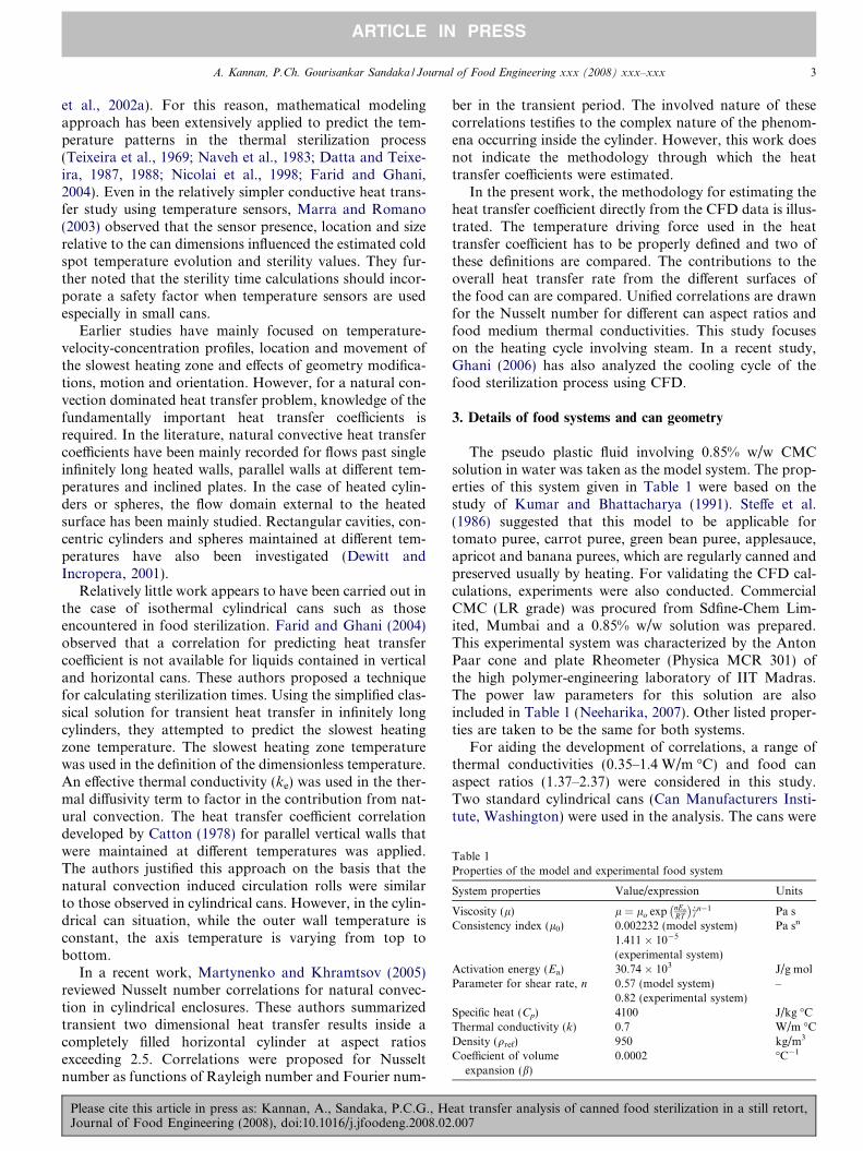
Table 1Properties of the model and experimental food system

System properties Value/expression Units

Viscosity (l) l ¼ lo exp nEa

RT

� �_cn�1 Pa s

Consistency index (l0) 0.002232 (model system) Pa sn

1.411 � 10�5

(experimental system)Activation energy (Ea) 30.74 � 103 J/g molParameter for shear rate, n 0.57 (model system) –

0.82 (experimental system)Specific heat (Cp) 4100 J/kg �CThermal conductivity (k) 0.7 W/m �CDensity (qref) 950 kg/m3

Coefficient of volumeexpansion (b)

0.0002 �C�1

A. Kannan, P.Ch. Gourisankar Sandaka / Journal of Food Engineering xxx (2008) xxx–xxx 3

ARTICLE IN PRESS

et al., 2002a). For this reason, mathematical modelingapproach has been extensively applied to predict the tem-perature patterns in the thermal sterilization process(Teixeira et al., 1969; Naveh et al., 1983; Datta and Teixe-ira, 1987, 1988; Nicolai et al., 1998; Farid and Ghani,2004). Even in the relatively simpler conductive heat trans-fer study using temperature sensors, Marra and Romano(2003) observed that the sensor presence, location and sizerelative to the can dimensions influenced the estimated coldspot temperature evolution and sterility values. They fur-ther noted that the sterility time calculations should incor-porate a safety factor when temperature sensors are usedespecially in small cans.

Earlier studies have mainly focused on temperature-velocity-concentration profiles, location and movement ofthe slowest heating zone and effects of geometry modifica-tions, motion and orientation. However, for a natural con-vection dominated heat transfer problem, knowledge of thefundamentally important heat transfer coefficients isrequired. In the literature, natural convective heat transfercoefficients have been mainly recorded for flows past singleinfinitely long heated walls, parallel walls at different tem-peratures and inclined plates. In the case of heated cylin-ders or spheres, the flow domain external to the heatedsurface has been mainly studied. Rectangular cavities, con-centric cylinders and spheres maintained at different tem-peratures have also been investigated (Dewitt andIncropera, 2001).

Relatively little work appears to have been carried out inthe case of isothermal cylindrical cans such as thoseencountered in food sterilization. Farid and Ghani (2004)observed that a correlation for predicting heat transfercoefficient is not available for liquids contained in verticaland horizontal cans. These authors proposed a techniquefor calculating sterilization times. Using the simplified clas-sical solution for transient heat transfer in infinitely longcylinders, they attempted to predict the slowest heatingzone temperature. The slowest heating zone temperaturewas used in the definition of the dimensionless temperature.An effective thermal conductivity (ke) was used in the ther-mal diffusivity term to factor in the contribution from nat-ural convection. The heat transfer coefficient correlationdeveloped by Catton (1978) for parallel vertical walls thatwere maintained at different temperatures was applied.The authors justified this approach on the basis that thenatural convection induced circulation rolls were similarto those observed in cylindrical cans. However, in the cylin-drical can situation, while the outer wall temperature isconstant, the axis temperature is varying from top tobottom.

In a recent work, Martynenko and Khramtsov (2005)reviewed Nusselt number correlations for natural convec-tion in cylindrical enclosures. These authors summarizedtransient two dimensional heat transfer results inside acompletely filled horizontal cylinder at aspect ratiosexceeding 2.5. Correlations were proposed for Nusseltnumber as functions of Rayleigh number and Fourier num-


ber in the transient period. The involved nature of thesecorrelations testifies to the complex nature of the phenom-ena occurring inside the cylinder. However, this work doesnot indicate the methodology through which the heattransfer coefficients were estimated.

In the present work, the methodology for estimating theheat transfer coefficient directly from the CFD data is illus-trated. The temperature driving force used in the heattransfer coefficient has to be properly defined and two ofthese definitions are compared. The contributions to theoverall heat transfer rate from the different surfaces ofthe food can are compared. Unified correlations are drawnfor the Nusselt number for different can aspect ratios andfood medium thermal conductivities. This study focuseson the heating cycle involving steam. In a recent study,Ghani (2006) has also analyzed the cooling cycle of thefood sterilization process using CFD.

3. Details of food systems and can geometry

The pseudo plastic fluid involving 0.85% w/w CMCsolution in water was taken as the model system. The prop-erties of this system given in Table 1 were based on thestudy of Kumar and Bhattacharya (1991). Steffe et al.(1986) suggested that this model to be applicable fortomato puree, carrot puree, green bean puree, applesauce,apricot and banana purees, which are regularly canned andpreserved usually by heating. For validating the CFD cal-culations, experiments were also conducted. CommercialCMC (LR grade) was procured from Sdfine-Chem Lim-ited, Mumbai and a 0.85% w/w solution was prepared.This experimental system was characterized by the AntonPaar cone and plate Rheometer (Physica MCR 301) ofthe high polymer-engineering laboratory of IIT Madras.The power law parameters for this solution are alsoincluded in Table 1 (Neeharika, 2007). Other listed proper-ties are taken to be the same for both systems.

For aiding the development of correlations, a range ofthermal conductivities (0.35–1.4 W/m �C) and food canaspect ratios (1.37–2.37) were considered in this study.Two standard cylindrical cans (Can Manufacturers Insti-tute, Washington) were used in the analysis. The cans were


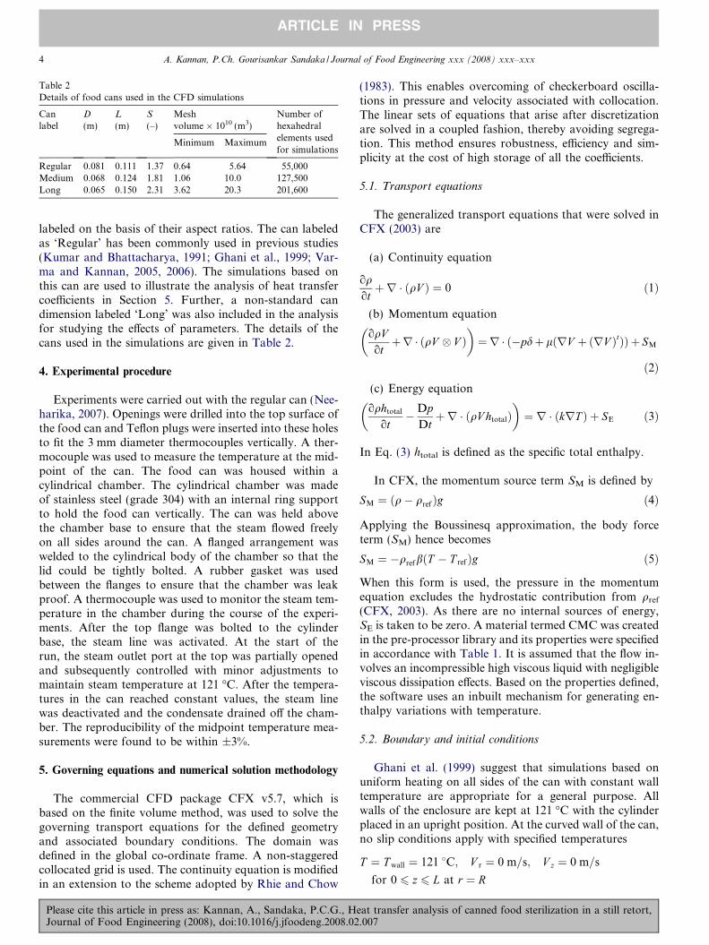
Table 2Details of food cans used in the CFD simulations

Canlabel

D

(m)L

(m)S

(–)Meshvolume � 1010 (m3)

Number ofhexahedralelements usedfor simulations

Minimum Maximum

Regular 0.081 0.111 1.37 0.64 5.64 55,000Medium 0.068 0.124 1.81 1.06 10.0 127,500Long 0.065 0.150 2.31 3.62 20.3 201,600


ARTICLE IN PRESS

labeled on the basis of their aspect ratios. The can labeledas ‘Regular’ has been commonly used in previous studies(Kumar and Bhattacharya, 1991; Ghani et al., 1999; Var-ma and Kannan, 2005, 2006). The simulations based onthis can are used to illustrate the analysis of heat transfercoefficients in Section 5. Further, a non-standard candimension labeled ‘Long’ was also included in the analysisfor studying the effects of parameters. The details of thecans used in the simulations are given in Table 2.

4. Experimental procedure

Experiments were carried out with the regular can (Nee-harika, 2007). Openings were drilled into the top surface ofthe food can and Teflon plugs were inserted into these holesto fit the 3 mm diameter thermocouples vertically. A ther-mocouple was used to measure the temperature at the mid-point of the can. The food can was housed within acylindrical chamber. The cylindrical chamber was madeof stainless steel (grade 304) with an internal ring supportto hold the food can vertically. The can was held abovethe chamber base to ensure that the steam flowed freelyon all sides around the can. A flanged arrangement waswelded to the cylindrical body of the chamber so that thelid could be tightly bolted. A rubber gasket was usedbetween the flanges to ensure that the chamber was leakproof. A thermocouple was used to monitor the steam tem-perature in the chamber during the course of the experi-ments. After the top flange was bolted to the cylinderbase, the steam line was activated. At the start of therun, the steam outlet port at the top was partially openedand subsequently controlled with minor adjustments tomaintain steam temperature at 121 �C. After the tempera-tures in the can reached constant values, the steam linewas deactivated and the condensate drained off the cham-ber. The reproducibility of the midpoint temperature mea-surements were found to be within ±3%.

5. Governing equations and numerical solution methodology

The commercial CFD package CFX v5.7, which isbased on the finite volume method, was used to solve thegoverning transport equations for the defined geometryand associated boundary conditions. The domain wasdefined in the global co-ordinate frame. A non-staggeredcollocated grid is used. The continuity equation is modifiedin an extension to the scheme adopted by Rhie and Chow


(1983). This enables overcoming of checkerboard oscilla-tions in pressure and velocity associated with collocation.The linear sets of equations that arise after discretizationare solved in a coupled fashion, thereby avoiding segrega-tion. This method ensures robustness, efficiency and sim-plicity at the cost of high storage of all the coefficients.

5.1. Transport equations

The generalized transport equations that were solved inCFX (2003) are

(a) Continuity equation

oqotþr � ðqV Þ ¼ 0 ð1Þ

(b) Momentum equation

oqVotþr � ðqV � V Þ

� �¼r � ð�pdþ lðrV þ ðrV ÞtÞÞ þ SM

ð2Þ(c) Energy equation

oqhtotal

ot�Dp

Dtþr � qV htotalð Þ

� �¼ r � ðkrT Þ þ SE ð3Þ

In Eq. (3) htotal is defined as the specific total enthalpy.

In CFX, the momentum source term SM is defined by

SM ¼ ðq� qrefÞg ð4Þ

Applying the Boussinesq approximation, the body forceterm (SM) hence becomes

SM ¼ �qrefbðT � T refÞg ð5Þ

When this form is used, the pressure in the momentumequation excludes the hydrostatic contribution from qref

(CFX, 2003). As there are no internal sources of energy,SE is taken to be zero. A material termed CMC was createdin the pre-processor library and its properties were specifiedin accordance with Table 1. It is assumed that the flow in-volves an incompressible high viscous liquid with negligibleviscous dissipation effects. Based on the properties defined,the software uses an inbuilt mechanism for generating en-thalpy variations with temperature.

5.2. Boundary and initial conditions

Ghani et al. (1999) suggest that simulations based onuniform heating on all sides of the can with constant walltemperature are appropriate for a general purpose. Allwalls of the enclosure are kept at 121 �C with the cylinderplaced in an upright position. At the curved wall of the can,no slip conditions apply with specified temperatures

T ¼ T wall ¼ 121 �C; V r ¼ 0 m=s; V z ¼ 0 m=s

for 0 6 z 6 L at r ¼ R



ARTICLE IN PRESS

At the top and bottom walls of the container, again no slipconditions apply with specified temperatures

T ¼ T wall ¼ 121 �C; V r ¼ 0 m=s; V z ¼ 0 m=s

for 0 6 r 6 R at z ¼ 0 and L

Initially the fluid is at rest and at a uniform initialtemperature

T 0 ¼ 40 �C; V r ¼ 0 m=s; V z ¼ 0 m=s

for 0 6 r 6 R and 0 6 z 6 L

The condensing steam is assumed to maintain a commonlyapplied constant temperature of 121 �C at all boundaries.This temperature is assumed to apply at the liquid bound-aries owing to the very small thermal resistance of the canmaterial. Further, the temperature at the liquid boundariesis assumed to reach this temperature from the initial condi-tions without any lag.

5.3. Mesh and time step details

CFD simulations, especially those involving transients,are time consuming even with faster processors. Exploitingthe axisymmetry, only a segment of the cylinder was used.The structured mesh option from CFX Build v 5.6 wasapplied. To resolve the rapid changes in velocities and tem-peratures near the walls, finer rectangular mesh wasapplied closer to the walls, which gradually gave way toincreasingly coarser ones towards the core. For the cylin-ders used in the study, the smallest element size was around0.3 mm, while the largest element size was near 1 mm in theradial direction. Along the axial direction, the mesh sizeswere between 1 and 2 mm. The total number of hexahedralelements in the domain and mesh volumes for each case isincluded in Table 2. The transient runs were carried out byadopting the step size-time relationship provided byKumar and Bhattacharya (1991). Upon doubling the timestep sizes, the results did not differ significantly. However,the earlier finer time step strategy was chosen.

The results from the structured meshes used here com-pared well with the earlier reported values for midpointtemperatures of Kumar and Bhattacharya (1991) as wellas from Varma and Kannan (2005). The unstructured meshscheme was used by Varma and Kannan (2005, 2006) intheir previous studies. A coarse structured mesh schemewas also investigated in the present work to study the effectof mesh sizes. For instance, a coarse mesh scheme wastested for the regular cylinder with 25,000 hexahedral ele-ments as against 55,000 hexahedral elements used in thefine mesh scheme. The element sizes were roughly 1.9 timeshigher along the radial direction with the minimum andmaximum mesh sizes being 0.6 mm and 2.3 mm. Theresults were not found to be in significant variance. How-ever, the refined mesh scheme whose details were shownin Table 2 was used in this work.

Finally, the axisymmetry condition was also verified bysimulating over the entire cylinder. No significant


azimuthal flow or variations in temperatures were encoun-tered. Detailed results of mesh independency studies areprovided elsewhere (Gourisankar, 2006). The simulationswere executed in the Intel Pentium (R) 4, 3.06 GHz and1 GB RAM with Windows XP platform. The CPU timefor the regular cylinder case for instance was estimated at1.2 h.

5.4. Solution methodology

The transient calculations were carried out using therobust and bounded first-order backward Euler scheme.CFX has the optional schemes of first order upwind differ-ence and numerical advection with specified blend factor.The blend factor may be varied between 0 and 1 to optbetween the first- and second-order schemes in order tocontrol numerical diffusion. However, these schemes arenot robust and non-physical overshoots and undershootsmay occur. Hence, the high-resolution scheme option,which maintains the blend factor as close as possible tounity without violating the boundedness principle, waschosen. In the present simulations, non-physical over-shoots or undershoots in the solution were not encoun-tered. Convergence criterion was fixed at residuals rootmean square (RMS) value lower than 10�4. The low Gras-hof numbers encountered during the entire course of simu-lations justified laminar flow conditions.

6. Results and discussion

6.1. Calculation of wall heat flux

At representative time steps, heat fluxes at the walls(sidewall, top and bottom surfaces) were determined usingthe CFX post processor. The wall heat flux at any givenheight on the curved surface is related to the temperaturegradient by the following equation:

qw ¼ koTor

��r¼R

ð6Þ

Temperature depends on both r and z and increases to-wards the curved wall, i.e. with increasing radial coordinater. The heat transfer coefficient is defined as follows:

qw ¼ hðT w � T bulkÞ ð7Þ

6.2. Estimation of suitable bulk temperature

Bird et al. (2002) observe that care should be taken tonote the definitions of the heat transfer coefficients whenusing treatises and handbooks. Many literature sourcesdo not clearly define the heat transfer coefficients. Toobtain the heat transfer coefficient from the heat flux(Eq. (7)), it is necessary first to define the reference or ‘bulk’temperature (Tbulk). For flow past submerged bodies, thebulk fluid temperature may be set as that of the infinite sur-roundings. For fluid flow through a conduit, cup mean


0

100

200

300

400

500

600

0 0.01 0.02 0.03 0.04 0.05 0.06 0.07 0.08 0.09 0.1 0.11

Z (m)

5.17 9.37 15.62 29.30 35.77

44.38 615. 76 1007. 20 1999. 90 2589

h(W

/m2

o C)

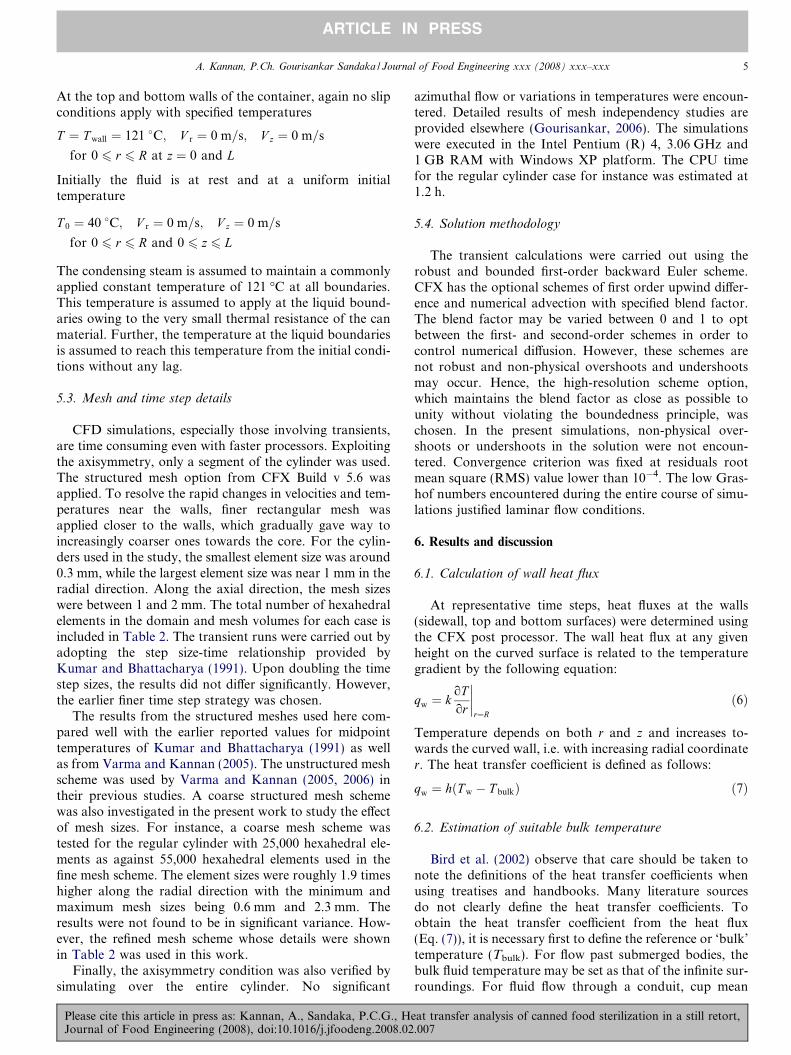
Fig. 1. Variation of the local heat transfer coefficients at different times (inseconds).


ARTICLE IN PRESS

mixing temperatures are often used. However, for the nat-ural convection engendered flow within the confines of afood can, the fluid flow is circulatory. However, the cupmean mixing temperature would not apply at a given crosssection because the net flow across the cross section wouldbe zero. Hence, it is possible to define a bulk temperature interms of absolute mass flow averaged temperature (hTMi)as given below

hT Mi ¼R R

0jvjzTr drR R

0jvjzr dr

ð8Þ

The heat flux from the vertical curved wall was estimated.Horizontal slice planes, across which the flow occurs, areconstructed at different locations along the curved wall.Nine equidistant slice planes are used and these are locatedat 11.11 millimeter intervals along the curved wall of theregular cylinder. The influence of the top and bottom wallswould be minimal especially for long cylinders. However, asimilar procedure, by constructing vertical planes, may notbe adopted for estimating the local heat transfer coeffi-cients at the top and bottom surfaces of the can. For thiscase, the method is fraught with uncertainties associatedwith heat transfer contributions not only from the topand bottom walls but from the curved wall as well. Thetemperature field would be influenced by heat flux fromthe curved wall as well as from the top and bottom sur-faces. This effect would be significant especially when thediameter of the cylinder is small relative to the height, i.e.for high aspect ratios. It would be then incorrect to calcu-late the local heat transfer coefficient based only on theheat flux contribution from the bottom or top surface.Hence, a more convenient definition of the heat transfercoefficient is necessary and it will be interesting to compareits predictions with the earlier proposed method.

It is also possible to base the mean heat transfer coeffi-cient on the volume-averaged temperature in the domain.The volume-averaged temperature is the temperature thatwould be obtained if the entire contents of the can wereto be mixed. The volume-averaged temperature is definedas shown below

hT Vi ¼R R R

V Tr dr dhdzR R RV r dr dhdz

ð9Þ

The heat transfer coefficients results based on both thesemethods are presented and compared in the next section.

6.3. Heat transfer coefficient based on the absolute mass flowaveraged temperature

The local heat transfer coefficient (hM) was estimatedusing Eq. (8) after constructing the horizontal slice planesas discussed in Section 5.3. Its variation along the axialdirection is plotted for different time steps as illustratedin Fig. 1. In this figure, it may be seen that each time stepthe heat transfer coefficient is nearly a constant along thevertical direction. There is a small increase near the top


and bottom walls due to heat transfer effects from thesesurfaces. The decline in heat transfer coefficients with timemay be attributed to leveling of temperature gradients inthe domain. This in turn was caused by conduction andnatural convective mixing. The heat transfer coefficientvaried from an initial value of nearly 500 W/m2 �C to only40 W/m2 �C at the final stages of the heating process.

The axially averaged heat transfer coefficient based onthe absolute mass flow averaged temperature ðhM

avgÞ isdefined by

hMavg ¼

R L0

hM dzL

ð10Þ

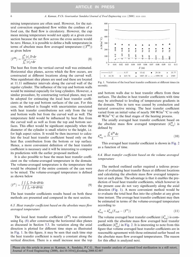
This averaged heat transfer coefficient is shown in Fig. 2as a function of time.

6.4. Heat transfer coefficient based on the volume averaged

temperature

The method outlined earlier required a tedious proce-dure of evaluating heat transfer fluxes at different locationsand calculating the absolute mass flow averaged tempera-ture at each plane. The advantage is that it enables the pre-diction of local heat transfer coefficients, which however inthe present case do not vary significantly along the axialdirection (Fig. 1). A more convenient method would beto evaluate the total heat flux into the cylinder at any giventime instant. The average heat transfer coefficient may thenbe estimated in terms of the volume-averaged temperatureaccording to

qVavg ¼ hV

avgðT wall � hT ViÞ ð11Þ

The volume averaged heat transfer coefficient ðhVavgÞ is com-

pared with the absolute mass flow averaged heat transfercoefficient ðhM

avgÞ in Fig. 2. It is interesting to note from thisfigure that volume averaged heat transfer coefficients are inreasonable agreement with those estimated earlier based onthe absolute mass flow averaged temperatures. The reasonfor this effect is analyzed next.


0

100

200

300

400

500

600

0 500 1000 1500 2000 2500 3000

time (s)

Mavgh V

avgh

h(W

/m2

o C)

Fig. 2. Comparison of average heat transfer coefficients based on averageabsolute mass flow average and volume averaged temperatures.

1

10

100

1000

10000

100000

1 10 100 1000 10000

time (s)

bottom top curved wall total

q w (W

/m2 )

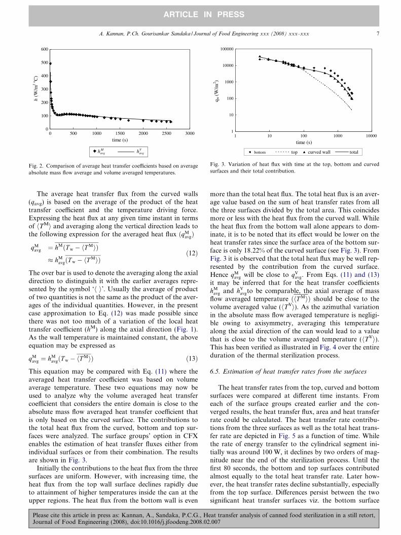
Fig. 3. Variation of heat flux with time at the top, bottom and curvedsurfaces and their total contribution.


ARTICLE IN PRESS

The average heat transfer flux from the curved walls(qavg) is based on the average of the product of the heattransfer coefficient and the temperature driving force.Expressing the heat flux at any given time instant in termsof hTMi and averaging along the vertical direction leads tothe following expression for the averaged heat flux ðqM

avgÞ

qMavg ¼ hMðT w � hT MiÞ

� hMavgðT w � hT MiÞ

ð12Þ

The over bar is used to denote the averaging along the axialdirection to distinguish it with the earlier averages repre-sented by the symbol ‘h i’. Usually the average of productof two quantities is not the same as the product of the aver-ages of the individual quantities. However, in the presentcase approximation to Eq. (12) was made possible sincethere was not too much of a variation of the local heattransfer coefficient (hM) along the axial direction (Fig. 1).As the wall temperature is maintained constant, the aboveequation may be expressed as

qMavg ¼ hM

avgðT w � hT MiÞ ð13Þ

This equation may be compared with Eq. (11) where theaveraged heat transfer coefficient was based on volumeaverage temperature. These two equations may now beused to analyze why the volume averaged heat transfercoefficient that considers the entire domain is close to theabsolute mass flow averaged heat transfer coefficient thatis only based on the curved surface. The contributions tothe total heat flux from the curved, bottom and top sur-faces were analyzed. The surface groups’ option in CFXenables the estimation of heat transfer fluxes either fromindividual surfaces or from their combination. The resultsare shown in Fig. 3.

Initially the contributions to the heat flux from the threesurfaces are uniform. However, with increasing time, theheat flux from the top wall surface declines rapidly dueto attainment of higher temperatures inside the can at theupper regions. The heat flux from the bottom wall is even


more than the total heat flux. The total heat flux is an aver-age value based on the sum of heat transfer rates from allthe three surfaces divided by the total area. This coincidesmore or less with the heat flux from the curved wall. Whilethe heat flux from the bottom wall alone appears to dom-inate, it is to be noted that its effect would be lower on theheat transfer rates since the surface area of the bottom sur-face is only 18.22% of the curved surface (see Fig. 3). FromFig. 3 it is observed that the total heat flux may be well rep-resented by the contribution from the curved surface.Hence qM

avg will be close to qVavg. From Eqs. (11) and (13)

it may be inferred that for the heat transfer coefficientshM

avg and hVavgto be comparable, the axial average of mass

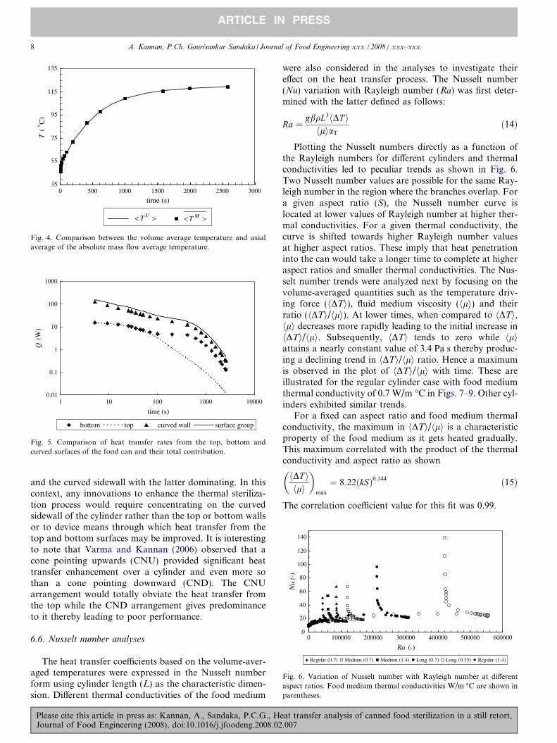
flow averaged temperature ðhT MiÞ should be close to thevolume averaged value (hTVi). As the azimuthal variationin the absolute mass flow averaged temperature is negligi-ble owing to axisymmetry, averaging this temperaturealong the axial direction of the can would lead to a valuethat is close to the volume averaged temperature (hTVi).This has been verified as illustrated in Fig. 4 over the entireduration of the thermal sterilization process.

6.5. Estimation of heat transfer rates from the surfaces

The heat transfer rates from the top, curved and bottomsurfaces were compared at different time instants. Fromeach of the surface groups created earlier and the con-verged results, the heat transfer flux, area and heat transferrate could be calculated. The heat transfer rate contribu-tions from the three surfaces as well as the total heat trans-fer rate are depicted in Fig. 5 as a function of time. Whilethe rate of energy transfer to the cylindrical segment ini-tially was around 100 W, it declines by two orders of mag-nitude near the end of the sterilization process. Until thefirst 80 seconds, the bottom and top surfaces contributedalmost equally to the total heat transfer rate. Later how-ever, the heat transfer rates decline substantially, especiallyfrom the top surface. Differences persist between the twosignificant heat transfer surfaces viz. the bottom surface


>< VT >< MT

35

55

75

95

115

135

0 500 1000 1500 2000 2500 3000

time (s)

T (

o C)

Fig. 4. Comparison between the volume average temperature and axialaverage of the absolute mass flow average temperature.

0.01

0.1

1

10

100

1000

1 10 100 1000 10000

time (s)

Q (

W)

bottom top curved wall surface group

Fig. 5. Comparison of heat transfer rates from the top, bottom andcurved surfaces of the food can and their total contribution.

0

20

40

60

80

100

120

140

0 100000 200000 300000 400000 500000 600000

Ra (-)

Nu

(-)

Regular (0.7) Medium (0.7) Medium (1.4) Long (0.7) Long (0.35) Regular (1.4)

Fig. 6. Variation of Nusselt number with Rayleigh number at differentaspect ratios. Food medium thermal conductivities W/m �C are shown inparentheses.


ARTICLE IN PRESS

and the curved sidewall with the latter dominating. In thiscontext, any innovations to enhance the thermal steriliza-tion process would require concentrating on the curvedsidewall of the cylinder rather than the top or bottom wallsor to device means through which heat transfer from thetop and bottom surfaces may be improved. It is interestingto note that Varma and Kannan (2006) observed that acone pointing upwards (CNU) provided significant heattransfer enhancement over a cylinder and even more sothan a cone pointing downward (CND). The CNUarrangement would totally obviate the heat transfer fromthe top while the CND arrangement gives predominanceto it thereby leading to poor performance.

6.6. Nusselt number analyses

The heat transfer coefficients based on the volume-aver-aged temperatures were expressed in the Nusselt numberform using cylinder length (L) as the characteristic dimen-sion. Different thermal conductivities of the food medium


were also considered in the analyses to investigate theireffect on the heat transfer process. The Nusselt number(Nu) variation with Rayleigh number (Ra) was first deter-mined with the latter defined as follows:

Ra ¼ gbqL3hDT ihliaT

ð14Þ

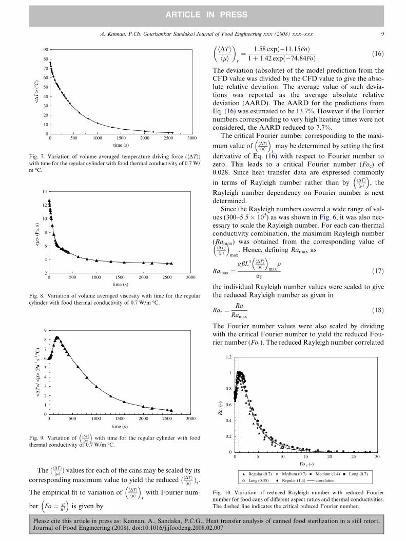
Plotting the Nusselt numbers directly as a function ofthe Rayleigh numbers for different cylinders and thermalconductivities led to peculiar trends as shown in Fig. 6.Two Nusselt number values are possible for the same Ray-leigh number in the region where the branches overlap. Fora given aspect ratio (S), the Nusselt number curve islocated at lower values of Rayleigh number at higher ther-mal conductivities. For a given thermal conductivity, thecurve is shifted towards higher Rayleigh number valuesat higher aspect ratios. These imply that heat penetrationinto the can would take a longer time to complete at higheraspect ratios and smaller thermal conductivities. The Nus-selt number trends were analyzed next by focusing on thevolume-averaged quantities such as the temperature driv-ing force (hDTi), fluid medium viscosity (hli) and theirratio (hDTi/hli). At lower times, when compared to hDTi,hli decreases more rapidly leading to the initial increase inhDTi/hli. Subsequently, hDTi tends to zero while hliattains a nearly constant value of 3.4 Pa s thereby produc-ing a declining trend in hDTi/hli ratio. Hence a maximumis observed in the plot of hDTi/hli with time. These areillustrated for the regular cylinder case with food mediumthermal conductivity of 0.7 W/m �C in Figs. 7–9. Other cyl-inders exhibited similar trends.

For a fixed can aspect ratio and food medium thermalconductivity, the maximum in hDTi/hli is a characteristicproperty of the food medium as it gets heated gradually.This maximum correlated with the product of the thermalconductivity and aspect ratio as shown

hDT ihli

� �max

¼ 8:22ðkSÞ0:144 ð15Þ

The correlation coefficient value for this fit was 0.99.


2

4

6

8

10

12

14

0 500 1000 1500 2000 2500 3000

time (s)

<>

(Pa

. s)

Fig. 8. Variation of volume averaged viscosity with time for the regularcylinder with food thermal conductivity of 0.7 W/m �C.

0

1

2

3

4

5

6

7

8

9

0 500 1000 1500 2000 2500 3000

time (s)

<ΔT

>/ <

> (

Pa-1

s-1

.o C)

Fig. 9. Variation of hDT ihli

� �with time for the regular cylinder with food

thermal conductivity of 0.7 W/m �C.

0

10

20

30

40

50

60

70

80

90

0 500 1000 1500 2000 2500 3000

time (s)

<ΔT

> (

o C)

Fig. 7. Variation of volume averaged temperature driving force (hDTi)with time for the regular cylinder with food thermal conductivity of 0.7 W/m �C.

0

0.2

0.4

0.6

0.8

1

1.2

0 5 10 15 20 25 30

Fo r (-)

Regular (0.7) Medium (0.7) Medium (1.4) Long (0.7)

Long (0.35) Regular (1.4) correlation

Ra r

(-)

Fig. 10. Variation of reduced Rayleigh number with reduced Fouriernumber for food cans of different aspect ratios and thermal conductivities.The dashed line indicates the critical reduced Fourier number.


ARTICLE IN PRESS

The ðhDT ihli Þ values for each of the cans may be scaled by its

corresponding maximum value to yield the reduced ðhDT ihli Þr.

The empirical fit to variation of hDT ihli

� �r

with Fourier num-

ber Fo ¼ atR2

� �is given by


hDT ihli

� �r

¼ 1:58 expð�11:15FoÞ1þ 1:42 expð�74:84FoÞ ð16Þ

The deviation (absolute) of the model prediction from theCFD value was divided by the CFD value to give the abso-lute relative deviation. The average value of such devia-tions was reported as the average absolute relativedeviation (AARD). The AARD for the predictions fromEq. (16) was estimated to be 13.7%. However if the Fouriernumbers corresponding to very high heating times were notconsidered, the AARD reduced to 7.7%.

The critical Fourier number corresponding to the maxi-

mum value of hDT ihli

� �r

may be determined by setting the first

derivative of Eq. (16) with respect to Fourier number tozero. This leads to a critical Fourier number (Foc) of0.028. Since heat transfer data are expressed commonly

in terms of Rayleigh number rather than by hDT ihli

� �, the

Rayleigh number dependency on Fourier number is nextdetermined.

Since the Rayleigh numbers covered a wide range of val-ues (300–5.5 � 105) as was shown in Fig. 6, it was also nec-essary to scale the Rayleigh number. For each can-thermalconductivity combination, the maximum Rayleigh number(Ramax) was obtained from the corresponding value ofhDT ihli

� �max

. Hence, defining Ramax as

Ramax ¼gbL3 hDT i

hli

� �max

q

aT

ð17Þ

the individual Rayleigh number values were scaled to givethe reduced Rayleigh number as given in

Rar ¼Ra

Ramax

ð18Þ

The Fourier number values were also scaled by dividingwith the critical Fourier number to yield the reduced Fou-rier number (For). The reduced Rayleigh number correlated



ARTICLE IN PRESS

with For as given in Eq. (19) and the fit with the data areshown in Fig. 10.

Rar ¼1:18 expð1:72ForÞ

1þ 0:75 expð2:02ForÞð19Þ

The critical reduced Fourier number is shown by the dashedline. The average absolute relative deviation (AARD) wasestimated to be 13%. However if the data correspondingto very high heating times (For > 10) were not considered,the AARD reduced to 7.5%. The Fourier number is the pri-

mary variable for correlating hDT ihli

� �r

and Nu. However, in

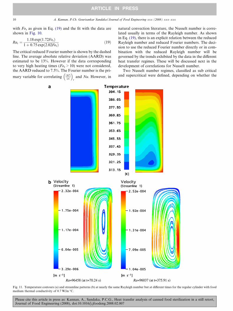
Fig. 11. Temperature contours (a) and streamline patterns (b) at nearly the sammedium thermal conductivity of 0.7 W/m �C.


natural convection literature, the Nusselt number is corre-lated usually in terms of the Rayleigh number. As shownin Eq. (19), there is an explicit relation between the reducedRayleigh number and reduced Fourier numbers. The deci-sion to use the reduced Fourier number directly or in com-bination with the reduced Rayleigh number will begoverned by the trends exhibited by the data in the differentheat transfer regimes. These will be discussed next in thedevelopment of correlations for Nusselt number.

Two Nusselt number regimes, classified as sub criticaland supercritical were defined, depending on whether the

e Rayleigh number but at different times for the regular cylinder with food


0

20

40

60

80

100

120

140

0 0.005 0.01 0.015 0.02 0.025 0.03

Fo (-)

Regular (0.7) Medium (0.7) Medium (1.4) Long (0.7)

Long (0.35) Regular (1.4) Theory Correlation

Nu S

(-)

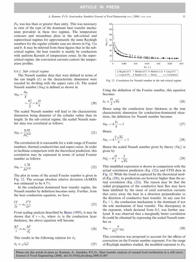
Fig. 12. Correlation for Nusselt number in the sub critical regime.


ARTICLE IN PRESS

For was less than or greater than unity. This was necessaryin view of the type of the dominant heat transfer mecha-nism prevalent in these two regimes. The temperaturecontours and streamlines plots in the sub-critical andsupercritical regimes for approximately the same Rayleighnumbers for the regular cylinder case are shown in Fig. 11aand b. It may be inferred from these figures that in the sub-critical regime, the heat transfer is mainly by conductionwith uniform Kernels of temperature zones. In the super-critical regime, the convection currents contort the temper-ature profiles.

6.6.1. Sub critical regime

The Nusselt number data that were defined in terms ofthe can length (L) as the characteristic dimension wererescaled by dividing with the aspect ratio (S). The scaledNusselt number (NuS) is defined as shown in

NuS ¼NuS

¼h L

kLD

¼ hDk

ð20Þ

The scaled Nusselt number will lead to the characteristicdimension being diameter of the cylinder rather than itslength. In the sub critical regime, the scaled Nusselt num-ber data was correlated as follows:

NuS ¼8:92

Fo0:45r

ð21Þ

The correlation fit is reasonable for a wide range of Fouriernumbers, thermal conductivities and aspect ratios. In orderto facilitate comparison with the theoretical prediction, thiscorrelation may be expressed in terms of actual Fouriernumber as follows:

NuS ¼1:78

Fo0:45ð22Þ

The plot in terms of the actual Fourier number is given inFig. 12. The average absolute relative deviation (AARD)was estimated to be 4.7%.

In the conduction dominated heat transfer regime, theNusselt number by definition becomes unity. Further, fromthe heat conduction equation, we have

oTot¼ aT

o2T

or2ð23Þ

From scaling analysis described by Bejan (1995), it may beshown that if r dT, where dT is the conduction layerthickness, the above equation will become

DTt� aT

DT

d2T

ð24Þ

This results in the following relation for dT

dT �ffiffiffiffiffiffiffiaTtp

ð25Þ


Using the definition of the Fourier number, this equationbecomes

dT �D2

ffiffiffiffiffiFop

ð26Þ

Hence using the conduction layer thickness as the truecharacteristic dimension for conduction-dominated situa-tions, the definition for Nusselt number becomes

NuC ¼ hdT

k¼ 1 ð27Þ

Hence

NuC ¼ hD2

ffiffiffiffiffiFop

k¼ 1 ð28Þ

Hence the scaled Nusselt number given by theory ðNu�SÞ isgiven by

Nu�S ¼ hDk¼ 2ffiffiffiffiffi

Fop ð29Þ

This simplified expression is shown in comparison with theactual correlation prediction (Eq. (22)) and CFD data inFig. 12. While the trend is captured by the theoretical mod-el (Eq. (29)), its predictions are however higher than the ac-tual correlation (Eq. (22)). The reason may be that theradial propagation of the conductive heat flux may havebeen inhibited by the onset of axial convection currentsthat carry away the heat in a direction perpendicular tothe direction of conductive heat transfer. In any case forFor < 1, the conduction mechanism is the dominant if notthe sole mechanism of heat transfer. The discrepancy inthe exponent, which deviated from 0.5, was further ana-lyzed. It was observed that a marginally better correlationfit could be obtained by expressing the scaled Nusselt num-ber as

NuS ¼a

Fo0:5�bRarr

ð30Þ

This correlation was proposed to account for the effects ofconvection on the Fourier number exponent. For the rangeof Rayleigh numbers studied, the modified exponent to For



ARTICLE IN PRESS

(as well as Fo) ranged only between 0.44 and 0.46. Hence,the simpler form given by Eqs. (21) and (22) was retained.

6.6.2. Supercritical regime

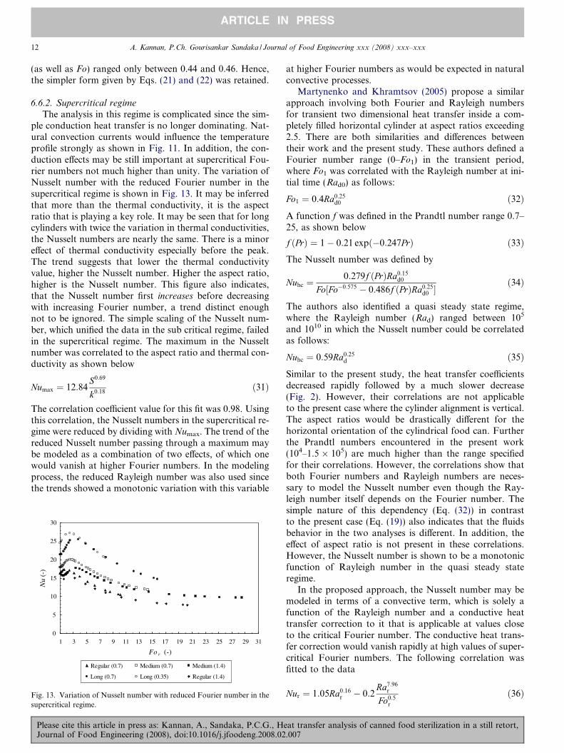
The analysis in this regime is complicated since the sim-ple conduction heat transfer is no longer dominating. Nat-ural convection currents would influence the temperatureprofile strongly as shown in Fig. 11. In addition, the con-duction effects may be still important at supercritical Fou-rier numbers not much higher than unity. The variation ofNusselt number with the reduced Fourier number in thesupercritical regime is shown in Fig. 13. It may be inferredthat more than the thermal conductivity, it is the aspectratio that is playing a key role. It may be seen that for longcylinders with twice the variation in thermal conductivities,the Nusselt numbers are nearly the same. There is a minoreffect of thermal conductivity especially before the peak.The trend suggests that lower the thermal conductivityvalue, higher the Nusselt number. Higher the aspect ratio,higher is the Nusselt number. This figure also indicates,that the Nusselt number first increases before decreasingwith increasing Fourier number, a trend distinct enoughnot to be ignored. The simple scaling of the Nusselt num-ber, which unified the data in the sub critical regime, failedin the supercritical regime. The maximum in the Nusseltnumber was correlated to the aspect ratio and thermal con-ductivity as shown below

Numax ¼ 12:84S0:69

k0:18ð31Þ

The correlation coefficient value for this fit was 0.98. Usingthis correlation, the Nusselt numbers in the supercritical re-gime were reduced by dividing with Numax. The trend of thereduced Nusselt number passing through a maximum maybe modeled as a combination of two effects, of which onewould vanish at higher Fourier numbers. In the modelingprocess, the reduced Rayleigh number was also used sincethe trends showed a monotonic variation with this variable

0

5

10

15

20

25

30

1 3 5 7 9 11 13 15 17 19 21 23 25 27 29 31

Fo r (-)

Regular (0.7) Medium (0.7) Medium (1.4)

Long (0.7) Long (0.35) Regular (1.4)

Nu

(-)

Fig. 13. Variation of Nusselt number with reduced Fourier number in thesupercritical regime.


at higher Fourier numbers as would be expected in naturalconvective processes.

Martynenko and Khramtsov (2005) propose a similarapproach involving both Fourier and Rayleigh numbersfor transient two dimensional heat transfer inside a com-pletely filled horizontal cylinder at aspect ratios exceeding2.5. There are both similarities and differences betweentheir work and the present study. These authors defined aFourier number range (0–Fo1) in the transient period,where Fo1 was correlated with the Rayleigh number at ini-tial time (Rad0) as follows:

Fo1 ¼ 0:4Ra0:25d0 ð32Þ

A function f was defined in the Prandtl number range 0.7–25, as shown below

f ðPrÞ ¼ 1� 0:21 expð�0:247PrÞ ð33ÞThe Nusselt number was defined by

Nuhc ¼0:279f ðPrÞRa0:15

d0

Fo½Fo�0:575 � 0:486f ðPrÞRa0:25d0

ð34Þ

The authors also identified a quasi steady state regime,where the Rayleigh number (Rad) ranged between 105

and 1010 in which the Nusselt number could be correlatedas follows:

Nuhc ¼ 0:59Ra0:25d ð35Þ

Similar to the present study, the heat transfer coefficientsdecreased rapidly followed by a much slower decrease(Fig. 2). However, their correlations are not applicableto the present case where the cylinder alignment is vertical.The aspect ratios would be drastically different for thehorizontal orientation of the cylindrical food can. Furtherthe Prandtl numbers encountered in the present work(104–1.5 � 105) are much higher than the range specifiedfor their correlations. However, the correlations show thatboth Fourier numbers and Rayleigh numbers are neces-sary to model the Nusselt number even though the Ray-leigh number itself depends on the Fourier number. Thesimple nature of this dependency (Eq. (32)) in contrastto the present case (Eq. (19)) also indicates that the fluidsbehavior in the two analyses is different. In addition, theeffect of aspect ratio is not present in these correlations.However, the Nusselt number is shown to be a monotonicfunction of Rayleigh number in the quasi steady stateregime.

In the proposed approach, the Nusselt number may bemodeled in terms of a convective term, which is solely afunction of the Rayleigh number and a conductive heattransfer correction to it that is applicable at values closeto the critical Fourier number. The conductive heat trans-fer correction would vanish rapidly at high values of super-critical Fourier numbers. The following correlation wasfitted to the data

Nur ¼ 1:05Ra0:16r � 0:2

Ra7:96r

Fo0:5r

ð36Þ



ARTICLE IN PRESS

The second term becomes insignificant at higher Fouriernumbers that correspond to lower values of the reducedRayleigh number (see Fig. 15). Hence, it may be seen thatat higher Fourier numbers, the Nusselt number simplifiesto

Nur ¼ 1:05Ra0:16r ð37Þ

The correlation produces a fit within ± 10% to the CFDnumerical data.

6.7. Validation of temperatures and heat flux data obtained

from CFD

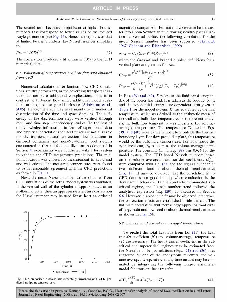
Numerical calculations for laminar flow CFD simula-tions are straightforward, as the governing transport equa-tions do not pose additional complications. This is incontrast to turbulent flow where additional model equa-tions are required to provide closure (Srinivasan et al.,2005). Hence, the error may arise mainly from numericaldiscretization of the time and space domains. The suffi-ciency of the discretization steps were verified throughmesh and time step independency studies. To the best ofour knowledge, information in form of experimental dataand empirical correlations for heat fluxes are not availablefor the transient natural convection flow situations inenclosed containers and non-Newtonian food systemsencountered in thermal food sterilization. As described inSection 4, experiments were conducted with a test systemto validate the CFD temperature predictions. The mid-point location was chosen for measurement to avoid endand wall effects. The measured temperatures were foundto be in reasonable agreement with the CFD predictionsas shown in Fig. 14.

Next, the mean Nusselt number values obtained fromCFD simulations of the actual model system was validated.If the vertical wall of the cylinder is approximated as anisothermal plate, then an appropriate literature correlationfor Nusselt number may be used for at least an order of

30

50

70

90

110

130

0 500 1000 1500 2000 2500 3000

Time (s)

Experiment CFD

T (

o C)

Fig. 14. Comparison between experimentally measured and CFD pre-dicted midpoint temperatures.


magnitude comparison. For natural convective heat trans-fer into a non-Newtonian fluid flowing steadily past an iso-thermal vertical surface the following correlation for themean Nusselt number has been suggested (Skelland,1967; Chhabra and Richardson, 1999)

NuVP ¼ CncðGrVPÞ1

2ðnþ1ÞðPrVPÞn

3nþ1 ð38Þwhere the Grashof and Prandtl number definitions for avertical plate are given as follows:

GrVP ¼q2Lnþ2½gbðT w � T 0Þ2�n

K2ð39Þ

PrVP ¼qCP

kKq

� � 21þn

L1�n1þnðLgbðT w � T 0ÞÞ

3ðn�1Þ2ð1þnÞ ð40Þ

In Eqs. (39) and (40), K refers to the fluid consistency in-dex of the power law fluid. It is taken as the product of l0

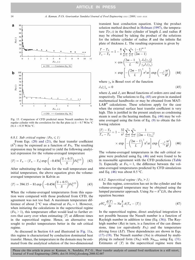
and the exponential temperature dependent term given inTable 1 for the model system. K was evaluated at the filmtemperature, which was defined as the arithmetic mean ofthe wall and bulk flow temperature. In the present analy-sis, the bulk flow temperature was chosen as the volume-averaged temperature. The temperature T0 used in Eqs.(39) and (40) refer to the temperature outside the thermalboundary layer. For flow past a flat plate, this temperaturewould be the bulk fluid temperature. For flow inside thecylindrical can, T0 is taken as the volume averaged tem-perature. The constant Cnc in Eq. (38) was 0.636 for themodel system. The CFD based Nusselt numbers basedon the volume averaged heat transfer coefficients ðhV

avgÞwere compared with Eq. (38) for the regular cylinder attwo different food medium thermal conductivities(Fig. 15). It may be observed that the correlation fit toCFD data is not good initially when conduction is thedominant mechanism. In the conduction-dominated subcritical regime, the Nusselt number trend followed theanalytical expression (Eq. (29)) as discussed in Section6.6. However, a reasonable fit may be observed later whenthe convection effects are established inside the can. Theflat plate correlation will increasingly apply for food cansof large radii and low food medium thermal conductivitiesas shown in Fig. 15b.

6.8. Estimation of the volume averaged temperatures

To predict the total heat flux from Eq. (11), the heattransfer coefficient (hV) and volume-averaged temperaturehTi are necessary. The heat transfer coefficient in the subcritical and supercritical regimes may be estimated fromthe Nusselt number correlations (Eqs. (21) and (36)). Assuggested by one of the anonymous reviewers, the vol-ume-averaged temperature at any time instant may be esti-mated by integrating the following lumped parametermodel for transient heat transfer

qVCpdhT i

dt¼ hVAðT w � hT iÞ ð41Þ


0

10

20

30

40

50

60

70

80

0 1 2 3 4 5 6 7 8 9 10 11

Fo r (-)

Fo r (-)

Nu

(-)

CFD Correlation (Eq. 38)

0

1020

30

40

5060

70

8090

100

0 1 2 3 4 5 6

Nu

(-)

CFD Correlation (Eq. 38)

a

b

Fig. 15. Comparison of CFD predicted mean Nusselt numbers for theregular cylinder with the correlation for the flat plate (a) k = 0.7 W/m �C(b) k = 0.35 W/m �C.


ARTICLE IN PRESS

6.8.1. Sub critical regime (For 6 1)

From Eqs. (20) and (21), the heat transfer coefficient(hV) may be expressed as a function of For. The resultingexpression may be integrated to yield the following analyt-ical expression for the volume-averaged temperature

hT i ¼ T w � ðT w � T 0Þ exp �0:454S þ 0:5

S

� �Fo0:55

r

� �ð42Þ

After substituting the values for the wall temperature andinitial temperature, the above equation gives the volume-averaged temperature in Kelvin as

hT i ¼ 394:15� 81 exp �0:454S þ 0:5

S

� �Fo0:55

r

� �ð43Þ

When the volume-averaged temperatures from this equa-tion were compared with those predicted from CFD, theagreement was not too bad. A maximum temperature dif-ference of about 2 �C was observed at For = 1. However,when initiating the calculations in the supercritical regime(For > 1), this temperature offset would lead to further er-rors that carry over when estimating hTi at different timesin the supercritical regime. Hence, an alternative wassought to predict temperatures better in the sub criticalregime.

As discussed in Section 6.6 and illustrated in Fig. 11a,this regime is characterized by conduction dominated heattransfer. Hence, the temperature in the domain may be esti-mated from the analytical solution of the two-dimensional


transient heat conduction equation. Using the productsolution method described in Holman (1997), the tempera-ture T(r,z) in the finite cylinder of length L and radius R

may be obtained by taking the product of the solutionsfor the infinite cylinder of radius R and the infinite flatplate of thickness L. The resulting expression is given by

T � T 0

T w � T 0

¼ 1� 8

p

X1m¼1

X1n¼1

ð�1Þmþ1

ð2m� 1Þ

� cos2m� 1

Lpz

� �J 0 cn

rR

� �cnJ 1ðcnÞ

� exp � 2m� 1

L

� �2

p2at

" #exp �c2

n

at

R2

� �ð44Þ

where cn is Bessel root of the function

J 0ðcÞn ¼ 0 ð45Þwhere J0 and J1 are Bessel functions of orders zero and onerespectively. The solutions to Eq. (45) are given in standardmathematical handbooks or may be obtained from MAT-LAB� calculations. These solutions apply for the casewhen the external surface heat transfer coefficient is veryhigh. This is justified in the present analyses as condensingsteam is used as the heating medium. Eq. (44) may be vol-ume averaged using the form of Eq. (9) to obtain the fol-lowing relation

hT i � T 0

T w � T 0

¼ 1� 32

p2

X1m¼1

X1n¼1

1

½ð2m� 1Þcn2

� exp � 2m� 1

L

� �2

p2at

" #exp �c2

n

at

R2

� �ð46Þ

The volume-averaged temperatures in the sub critical re-gime were predicted using Eq. (46) and were found to bein reasonable agreement with the CFD predictions (Table3). Especially at For = 1, the difference between the vol-ume-averaged temperatures predicted by CFD simulationsand Eq. (46) was about 0.5 �C.

6.8.2. Supercritical regime (For > 1)

In this regime, convection has set in the cylinder and thevolume-averaged temperature may be obtained using thelumped parameter approach. Using Nu = hVL/k, the aboveequation becomes

qVCpdhT i

dt¼ Nu

kL

AðT w � hT iÞ ð47Þ

In the supercritical regime, direct analytical integration isnot possible because the Nusselt number is a function ofRayleigh number in addition to time (Eq. (36)). The Ray-leigh number (Ra) in turn, is a function of the can dimen-sions, time (or equivalently For) and the temperaturedriving force (DT). These dependencies are shown in Eqs.(17)–(19). The Nusselt number (Nu) is obtained by multi-plying its reduced form (Nur) with Numax using Eq. (31).Estimates of hTi in the supercritical regime were then


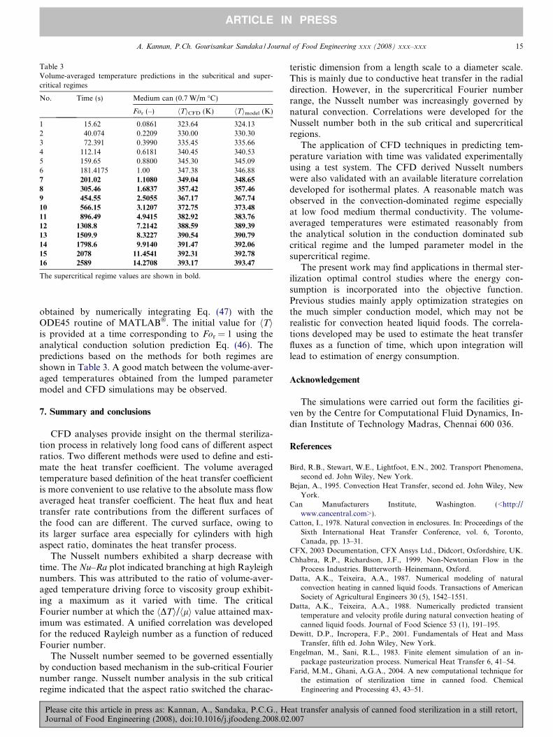
Table 3Volume-averaged temperature predictions in the subcritical and super-critical regimes

No. Time (s) Medium can (0.7 W/m �C)

For (–) hTiCFD (K) hTimodel (K)

1 15.62 0.0861 323.64 324.132 40.074 0.2209 330.00 330.303 72.391 0.3990 335.45 335.664 112.14 0.6181 340.45 340.535 159.65 0.8800 345.30 345.096 181.4175 1.00 347.38 346.887 201.02 1.1080 349.04 348.65

8 305.46 1.6837 357.42 357.46

9 454.55 2.5055 367.17 367.74

10 566.15 3.1207 372.75 373.48

11 896.49 4.9415 382.92 383.76

12 1308.8 7.2142 388.59 389.39

13 1509.9 8.3227 390.54 390.79

14 1798.6 9.9140 391.47 392.06

15 2078 11.4541 392.31 392.78

16 2589 14.2708 393.17 393.47

The supercritical regime values are shown in bold.


ARTICLE IN PRESS

obtained by numerically integrating Eq. (47) with theODE45 routine of MATLAB�. The initial value for hTiis provided at a time corresponding to For = 1 using theanalytical conduction solution prediction Eq. (46). Thepredictions based on the methods for both regimes areshown in Table 3. A good match between the volume-aver-aged temperatures obtained from the lumped parametermodel and CFD simulations may be observed.

7. Summary and conclusions

CFD analyses provide insight on the thermal steriliza-tion process in relatively long food cans of different aspectratios. Two different methods were used to define and esti-mate the heat transfer coefficient. The volume averagedtemperature based definition of the heat transfer coefficientis more convenient to use relative to the absolute mass flowaveraged heat transfer coefficient. The heat flux and heattransfer rate contributions from the different surfaces ofthe food can are different. The curved surface, owing toits larger surface area especially for cylinders with highaspect ratio, dominates the heat transfer process.

The Nusselt numbers exhibited a sharp decrease withtime. The Nu–Ra plot indicated branching at high Rayleighnumbers. This was attributed to the ratio of volume-aver-aged temperature driving force to viscosity group exhibit-ing a maximum as it varied with time. The criticalFourier number at which the hDTi/hli value attained max-imum was estimated. A unified correlation was developedfor the reduced Rayleigh number as a function of reducedFourier number.

The Nusselt number seemed to be governed essentiallyby conduction based mechanism in the sub-critical Fouriernumber range. Nusselt number analysis in the sub criticalregime indicated that the aspect ratio switched the charac-


teristic dimension from a length scale to a diameter scale.This is mainly due to conductive heat transfer in the radialdirection. However, in the supercritical Fourier numberrange, the Nusselt number was increasingly governed bynatural convection. Correlations were developed for theNusselt number both in the sub critical and supercriticalregions.

The application of CFD techniques in predicting tem-perature variation with time was validated experimentallyusing a test system. The CFD derived Nusselt numberswere also validated with an available literature correlationdeveloped for isothermal plates. A reasonable match wasobserved in the convection-dominated regime especiallyat low food medium thermal conductivity. The volume-averaged temperatures were estimated reasonably fromthe analytical solution in the conduction dominated subcritical regime and the lumped parameter model in thesupercritical regime.

The present work may find applications in thermal ster-ilization optimal control studies where the energy con-sumption is incorporated into the objective function.Previous studies mainly apply optimization strategies onthe much simpler conduction model, which may not berealistic for convection heated liquid foods. The correla-tions developed may be used to estimate the heat transferfluxes as a function of time, which upon integration willlead to estimation of energy consumption.

Acknowledgement

The simulations were carried out form the facilities gi-ven by the Centre for Computational Fluid Dynamics, In-dian Institute of Technology Madras, Chennai 600 036.

References

Bird, R.B., Stewart, W.E., Lightfoot, E.N., 2002. Transport Phenomena,second ed. John Wiley, New York.

Bejan, A., 1995. Convection Heat Transfer, second ed. John Wiley, NewYork.

Can Manufacturers Institute, Washington. (<http://www.cancentral.com>).

Catton, I., 1978. Natural convection in enclosures. In: Proceedings of theSixth International Heat Transfer Conference, vol. 6, Toronto,Canada, pp. 13–31.

CFX, 2003 Documentation, CFX Ansys Ltd., Didcort, Oxfordshire, UK.Chhabra, R.P., Richardson, J.F., 1999. Non-Newtonian Flow in the

Process Industries. Butterworth–Heinemann, Oxford.Datta, A.K., Teixeira, A.A., 1987. Numerical modeling of natural

convection heating in canned liquid foods. Transactions of AmericanSociety of Agricultural Engineers 30 (5), 1542–1551.

Datta, A.K., Teixeira, A.A., 1988. Numerically predicted transienttemperature and velocity profile during natural convection heating ofcanned liquid foods. Journal of Food Science 53 (1), 191–195.

Dewitt, D.P., Incropera, F.P., 2001. Fundamentals of Heat and MassTransfer, fifth ed. John Wiley, New York.

Engelman, M., Sani, R.L., 1983. Finite element simulation of an in-package pasteurization process. Numerical Heat Transfer 6, 41–54.

Farid, M.M., Ghani, A.G.A., 2004. A new computational technique forthe estimation of sterilization time in canned food. ChemicalEngineering and Processing 43, 43–51.


http://www.cancentral.com

http://www.cancentral.com


ARTICLE IN PRESS

Ghani, A.G.A., 2006. A computer simulation of heating and coolingliquid food during sterilization process using computational fluiddynamics. Association for Computing Machinery New ZealandBulletin, 2(3), ISSN: 1176-9998.

Ghani, A.G.A., Farid, M.M., Chen, X.D., Richards, P., 1999. Numericalsimulation of natural convection heating of canned food usingcomputational fluid dynamics. Journal of Food Engineering 41, 55–64.

Ghani, A.G.A., Farid, M.M., Chen, X.D., 2002a. Theoretical andexperimental investigation of the thermal inactivation of Bacillus

stearothermophilus in food pouches. Journal of Food Engineering 51,221–228.

Ghani, A.G.A., Farid, M.M., Chen, X.D., 2002b. Theoretical andexperimental investigation of the thermal destruction of vitamin C infood pouches. Computers and Electronics in Agriculture 34, 129–143.

Ghani, A.G.A., Farid, M.M., Chen, X.D., 2002c. Numerical simulation oftransient temperature and velocity profiles in a horizontal can duringsterilization using computational fluid dynamics. Journal of FoodEngineering 51, 77–83.

Ghani, A.G.A., Farid, M.M., Zarrouk, S.J., 2003. The effect of canrotation on the thermal sterilization of liquid food using computa-tional fluid dynamics. Journal of Food Engineering 57, 9–16.

Gourisankar, S.P.Ch., 2006. Heat transfer analysis in canned foodsterilization. M. Tech. Project Report, IIT Madras.

Holman, J.P., 1997. Heat Transfer, eighth ed. McGraw-Hill, New York.Kumar, A., Bhattacharya, M., Blaylock, J., 1990. Numerical simulation of

natural convection heating of canned thick viscous liquid foodproduct. Journal of Food Science 55 (5), 1401–1411.

Kumar, A., Bhattacharya, M., 1991. Transient temperature and velocityprofiles in a canned non-Newtonian liquid food during sterilization ina still-cook retort. International Journal of Heat and Mass Transfer 34(4–5), 1083–1096.

Marra, F., Romano, V., 2003. A mathematical model to study theinfluence of wireless temperature sensor during assessment of cannedfood sterilization. Journal of Food Engineering 59 (2–3), 245–252.


Martynenko, O.G., Khramtsov, P.P., 2005. Free Convective HeatTransfer. Springer, New York.

Naveh, D., Kopelman, I.J., Pflug, I.J., 1983. The finite element method inthermal processing of foods. Journal of Food Science 48, 1086.

Neeharika, K., 2007. CFD simulations and experimental analysis ofcanned food sterilization. M.Tech. Project Report, IIT Madras.

Nicolai, B.M., Verboven, B., Scheerlinck, N., De Baerdemacker, J., 1998.Numerical analysis of the propagation of random parameter fluctu-ations in time and space during thermal food processes. Journal ofFood Engineering 38, 259–278.

Rhie, C.M., Chow, W.L., 1983. Numerical study of the turbulent flow pastan airfoil with trailing edge separation. AIAA Journal 21, 1527–1532.

Skelland, A.H.P., 1967. Non-newtonian Flow and Heat Transfer. Wiley,New York.

Srinivasan, R., Jayanti, S., Kannan, A., 2005. Effect of Taylor vortices onmass transfer from a rotating cylinder. AIChE Journal 51 (11), 2885–2898.

Steffe, J.F., Mohamed, I.O., Ford, E.W., 1986. Rheological properties offluid foods: data compilation. In: Okos, M.R. (Ed.), Physical andChemical Properties of Foods. American Society of AgriculturalEngineering, St. Joseph, MI.

Teixeira, A.A., Dixon, J.R., Zahradnik, J.W., Zinsmeister, G.E., 1969.Computer optimization of nutrient retention in thermal processing ofconduction-heated foods. Food Technology 23 (6), 134–140.

Varma, M.N., Kannan, A., 2005. Enhanced food sterilization throughinclination of the container walls and geometry modifications.International Journal of Heat and Mass Transfer 48 (18), 3753–3762.

Varma, M.N., Kannan, A., 2006. CFD studies on natural convectiveheating of canned food in conical and cylindrical containers. Journalof Food Engineering 77, 1024–1036.

Zechman, L.G., Pflug, I.J., 1989. Location of the slowest heating zone fornatural convection heating fluids in metal containers. Journal of FoodScience 54, 205–229, 226.


Download - Heat transfer analysis of canned food sterilization in a ...»¹ thuật ổn định... · Heat transfer analysis of canned food sterilization in a still retort A. Kannan*, P.Ch

Top Related