HERPETOFAUNA SPECIES CLASSIFICATION FROM CAMERA TRAP IMAGES
USING DEEP NEURAL NETWORK FOR CONSERVATION MONITORING
by
Sazida Binta Islam, B.Sc.
A thesis submitted to the Graduate Council of
Texas State University in partial fulfillment
of the requirements for the degree of
Master of Science
with a Major in Engineering
December 2020
Committee Members:
Damian Valles, Chair
Michael Forstner
William Stapleton

COPYRIGHT
by
Sazida Binta Islam
2020

FAIR USE AND AUTHOR’S PERMISSION STATEMENT
Fair Use
This work is protected by the Copyright Laws of the United States (Public Law 94-553,
section 107). Consistent with fair use as defined in the Copyright Laws, brief quotations
from this material are allowed with proper acknowledgement. Use of this material for
financial gain without the author’s express written permission is not allowed.
Duplication Permission
As the copyright holder of this work I, Sazida Binta Islam, authorize duplication of this
work, in whole or in part, for educational or scholarly purposes only.

DEDICATION
To my parents; a source of strength, endless support, and encouragement.
v
ACKNOWLEDGEMENTS
I would like to express my deep and sincere gratitude to Dr. Michael Forstner, the
Department of Biology, Texas State University for providing me the opportunity to work
in the promising research project. I feel privileged to learn and gather experiences under
his guidance and assistance.
No word is enough to convey my gratitude to my supervisor, Professor Dr.
Damian Valles. His persistence, solid advices and encouragement empowered me to
carry out the research process. The weekly meetings and discussions always leave me
with a direction, especially during the hard times I faced while struggling with research
work.
I also express thank to my thesis committee member, Dr. William Stapleton for
his time and insightful advice throughout the project. I am indebted to Dr. Vishu
Viswanathan, graduate program advisor for his excellent advice, constructive criticism,
and support throughout my graduate program.
I would like to acknowledge the researchers of Texas A&M University for
providing me camera trap data with labeling. Special thanks are given to the Ingram
School of Engineering of Texas State University for providing necessary learning
facilities, a great academic environment, along with essential laboratory arrangements.
Completion of my master's program would not have been so pleasant without the
companionship of my classmates. Specially, I am grateful to Shafinaz, Rezwan, Purvesh
for offering an ultimate comfort zone from the beginning of the master’s program, during
vi
the summer ‘Toad Call Mass Production’ project, till the end of my thesis work. I am also
glad to be a part of HiPE group, and introducing with such ambitious, warm-hearted
people with mixed backgrounds and specialties. I would like to say thanks to my friend
Otto Randolph, Jr. and his parents Mr. and Mrs. Randolph, for their affection and prayers.
I really appreciate their welcoming gesture during the time when I was trying to cope
with the new environment.
My deepest gratitude goes to my caring, loving, and compassionate husband,
Toufiqul Haque. When times get tough, your assistance and tolerance are much
appreciated and duly remarked. Most importantly, to my parents and parents’ in-laws – I
am forever grateful for unconditional prayer, inspiration, and assurance.
Lastly, my gratitude also extends to the members of Bangladesh Student
Association (BSA) at Texas State University for the endless generosity, and support I
received throughout these past two years along with all the precious moments that I got to
share.
vii
TABLE OF CONTENTS
Page
ACKNOWLEDGEMENTS ................................................................................................v
LIST OF TABLES ...............................................................................................................x
LIST OF FIGURES .......................................................................................................... xi
ABSTRACT ......................................................................................................................xv
CHAPTERS
1. INTRODUCTION ..............................................................................................1
1.1 Motivation of The Research Work ..............................................................1
1.2 Camera Traps in Wildlife Monitoring .........................................................3
1.3 Camera Traps in Herpetofauna Observation ................................................4
1.4 Challenges with Camera Trap Images .........................................................6
1.5 Camera Trap Data Processing with DCNN .................................................7
1.6 Thesis Outline ..............................................................................................8
2. BACKGROUND ................................................................................................9
2.1 Camera Trap Project Initialization by Texas State University ...................9
2.2 Citizen Science Projects ............................................................................10
2.3 Pre-trained Deep Learning Models ............................................................11
3. LITERATURE REVIEW ..................................................................................13
3.1 Species Identification Using Feature Extractor and Classifier .................13
3.2 Camera Trap Dataset with Deep Neural Network ....................................14
3.3 Target Species Recognition Using Deep Neural Network .......................16
3.4 Thesis Contributions .................................................................................17
4. THESIS IMPLEMENTATION STRATEGY ..................................................19
viii
5. DATASET ........................................................................................................23
5.1 Online Dataset (Phase One) ......................................................................23
5.1.1 Data Accumulation ....................................................................23
5.1.2 Specifications of Online Dataset ................................................24
5.2 Camera Trap Dataset (Phase Two) ............................................................26
5.2.1 Data Accumulation ....................................................................26
5.2.2 Specifications of Camera Trap Dataset ......................................28
6. DEEP LEARNING ............................................................................................31
6.1 Artificial Neural Network .........................................................................31
6.2 Deep Neural Network for Image Processing ............................................34
6.3 The Architecture of Deep Convolutional Neural Network .......................36
6.3.1 Building Block of Convolution Layer .......................................37
6.4 Regularization Methods ............................................................................41
7. METHODOLOGY ............................................................................................43
7.1 Data Preprocessing ....................................................................................43
7.1.1 Cleaning and Scaling .................................................................43
7.1.2 Oversampling ..............................................................................43
7.1.3 Augmentation .............................................................................45
7.1.4 Data Partitioning ........................................................................50
7.2 CNN Model Configuration .......................................................................52
7.2.1 Model Architecture for Phase One (Online Dataset) .................54
7.2.2 Model Architecture for Phase Two (Camera Trap Dataset) ......55
7.3 Optimizing the CNN Model ......................................................................57
7.4 Computational Tools and Environment ....................................................58
8. EXPERIMENT AND RESULT ANALYSIS ....................................................59
8.1 Experiment and Result Analysis for Phase One (Online Dataset) ............59
8.2 Experiment and Result Analysis for Phase Two (Camera Trap Dataset) ..65
8.2.1 Performance Evaluation of CNN-1 (Without Augmentation) ...67
8.2.2 Performance Evaluation of CNN-2 (With Augmentation) ........71
8.2.2.1 Attempts to Reduce Overfitting for CNN-2 .................76
ix
8.3 Discussion and Findings ...........................................................................79
9. CONCLUSION AND FUTURE WORK .........................................................84
APPENDIX SECTION .....................................................................................................86
REFERENCES .................................................................................................................91
x
LIST OF TABLES
Table Page
1. Percentages of camera trap publication focused on certain group of species from 226
sample study................................................................................................................5
2. Camera trap data of toad/frog, lizard, snake with their variety of taxon provided for
phase two dataset including data quantity for each target group .............................27
3. Several augmentation techniques used in CNN-2 model using Keras
ImageDataGenerator .................................................................................................47
4. Balanced dataset partitioning of online images .............................................................51
5. Balanced dataset partitioning for CNN-1 of camera trap images ..................................51
6. Balanced dataset partitioning for CNN-2 of camera trap images ..................................51
7. The overall classification result of CNN-1 and CNN-2 models for online dataset .......64
8. The overall classification results of CNN-1 models for camera trap dataset ................69
xi
LIST OF FIGURES
Figure Page
1. The percentage of threats by category impacting terrestrial reptiles estimated from
1,500 random sample from all over the world. ...........................................................2
2. (a) A camera trap setup in Bastrop County, Texas, USA, (b) Compact T70 Camera that
has been used to collect image data in Bastrop County, Texas ..................................4
3. (a) An example of drift fence setup deployed in Bastrop County, Texas, and (b) a
snake is passing through a drift fence .........................................................................6
4. Some of the challenging pictures from camera trap data, (a) night vision image of toad
having lighting brightness variation, (b) a lizard image having natural camouflage,
(c) image of a snake displaying partial body in highly cluttered background, and (d)
target species is very small to detect in background. ..................................................7
5. An overall workflow diagram of the research work having four major steps of image
classification procedure using DCNN algorithm. .......................................................8
6. Performance improvement of winning participants of ILSVRC2010-2014 competitions
for three tasks; Image classification, Single-object localization, and Object detection
illustrating the reduction of error for 1.2 million training images having 1000 object
categories ..................................................................................................................12
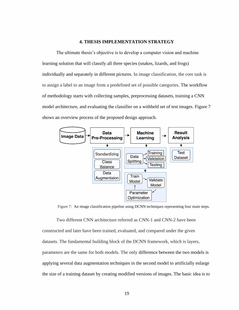
7. An image classification pipeline using DCNN techniques representing four
main steps..................................................................................................................19
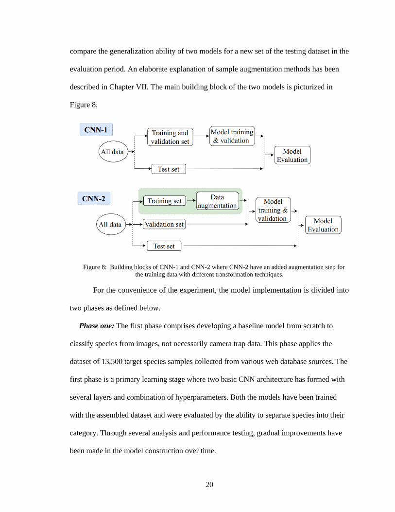
8. Building blocks of CNN-1 and CNN-2 where CNN-2 have an added augmentation
step for the training data with different transformation techniques. .........................20
9. Thesis implementation strategy overview for phase one and phase two that will be
implemented for two models (CNN-1 and CNN-2) .................................................22
10. Samples of (a) snake, (b) lizard, (c) frog/toad images collected from Pixabay,
Unsplash, and Caltech database ................................................................................25
11. Samples of (a) frog/toad, (b) snake, (c) lizard images from phase one dataset
presenting challenges such as confusing body color with nature having high
camouflage effect. .....................................................................................................25
xii
12. Samples of (a) frog/toad, (b) snake, (c) lizard images from phase one dataset
showing partially body size and occlusion by leaf or background ...........................25
13. Samples of (a) frog/toad, (b) snake, (c) lizard images from phase one dataset
displaying inter class similarities of species .............................................................26
14. An example of camera trap design deployed in longleaf pine habitat, Texas .............26
15. Samples of frog/toad from camera trap images having different challenges such as
small body size, cluttered background, confusing body color with nature, or hiding
body part behind leaf ................................................................................................29
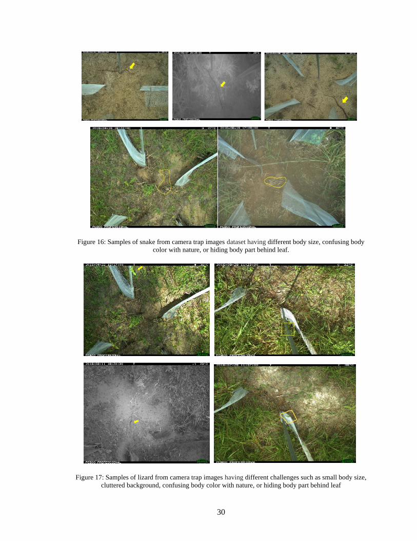
16. Samples of snake from camera trap images having different body size, confusing
body color with nature, or hiding body part behind leaf...........................................30
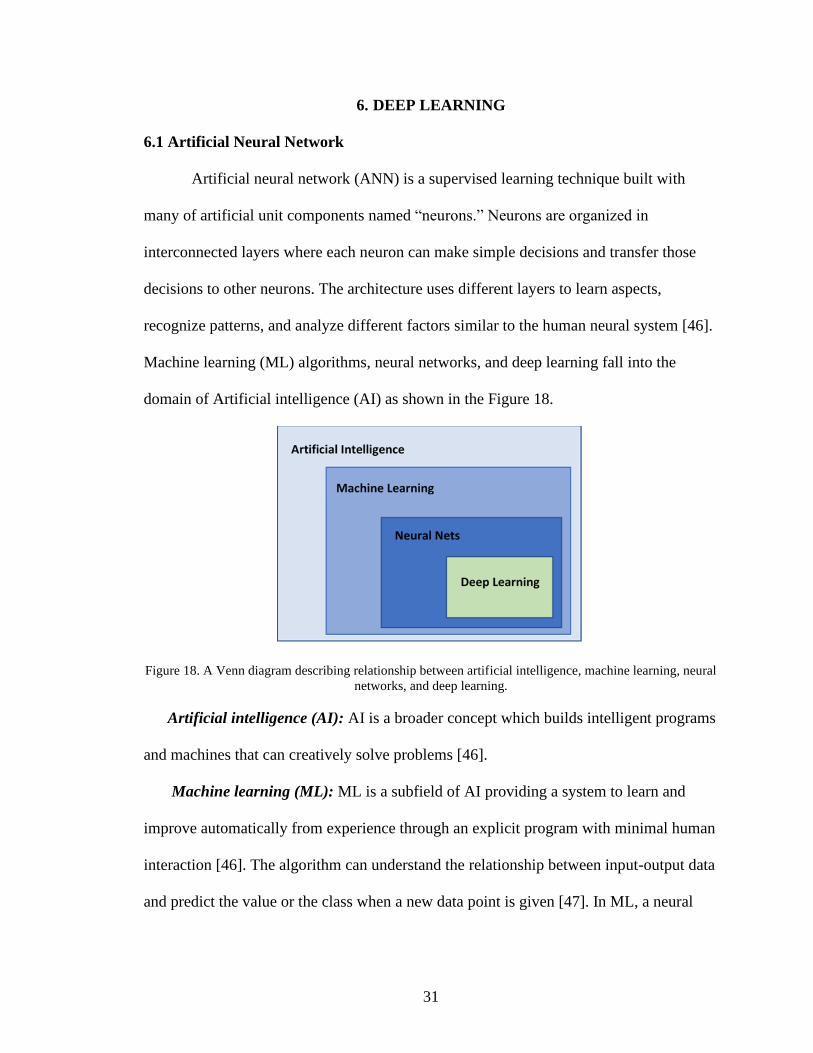
17. Samples of lizard from camera trap images having different challenges such as small
body size, cluttered background, confusing body color with nature, or hiding body
part behind leaf .........................................................................................................30
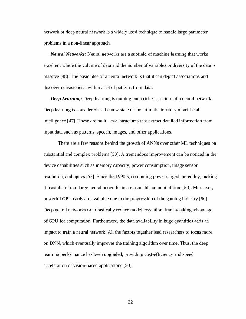
18. A Venn diagram describing relationship between artificial intelligence, machine
learning, neural networks, and deep learning ...........................................................31
19. Illustration of a biological neuron (left) and its mathematical model (right) ..............33
20. Neural network architectures with neurons and layers ................................................34
21. Up: Traditional images classification process by applying hand-designed feature
extraction algorithms followed by training a machine learning classifier. Down:
Deep learning approach of stacking layers that automatically learn more intricate,
abstract, and discriminating features. ........................................................................35
22. Stacking layers on top of each other that automatically learn more intricate, abstract,
and discriminating patterns in deep learning approach.............................................36
23. A CNN architecture to classify different type of vehicles using a set of layers where
the convolution and pooling layers pull out patterns and the fully connected layer
does classification by mapping the extracted features into final output ...................37
24. The mathematical operation in a convolutional layer where each filter convolves over
the input volume producing stack of feature maps ...................................................38
xiii
25. A movement of filters in the input matrix with a stride size is 2. ................................39
26. Plots of different activation functions with their computation behavior .....................39
27. Pictorial representation of max pooling and average pooling .....................................40
28. Pictorial representation of drop out layers ...................................................................42
29. Early stopping breaks the training procedure after reaching a particular accuracy/loss
score ..........................................................................................................................42
30. An illustration of balancing samples of all species by oversampling snake and toad
images .......................................................................................................................44
31. On-the-fly augmentation process in CNN-2 using image batch manipulations ..........47
32. Several augmentation examples applied in CNN-2 to transform images in training
phase .........................................................................................................................48
33. An overall concept of training and testing processes of a DCNN recognition
framework. ................................................................................................................52
34. An example of four layers CONV architecture for snake, lizard, and toad
classification .............................................................................................................53
35. The accuracy and loss curves (training and validation) during the 200-epoch training
process for the final CNN-1 model ...........................................................................61
36. The accuracy and loss curves (training and validation) during the 250-epoch training
process for the final CNN-2 model ...........................................................................61
37. Confusion matrix of Snake vs. Toad experiment (a) for CNN-1 and
(b) for CNN-2 ...........................................................................................................62
38. The accuracy, loss curves (training and validation), and confusion matrix of CNN-1
model for snake, toad and lizard classification .........................................................63
39. The accuracy, loss curves (training and validation), and confusion matrix of CNN-2
model for snake, toad and lizard classification .........................................................63
xiv
40. (a) The accuracy, loss curves (training and validation) with respect to the number of
epochs, and (b) confusion matrix of the final CNN-1 model for toad vs background
of camera trap images ...............................................................................................68
41. (a) The accuracy, loss curves (training and validation) with respect to the number of
epochs, and (b) confusion matrix of the final CNN-1 model for lizard vs
background of camera trap images ...........................................................................68
42. (a) The accuracy, loss curves (training and validation) with respect to the number of
epochs, and (b) confusion matrix of the final CNN-1 model for snake vs
background of camera trap images ...........................................................................68
43 (a) The accuracy, loss curves (training and validation) with respect to the number
of epochs, and (b) confusion matrix of the final CNN-1 model for all three species
of camera trap images ...............................................................................................70
44. (a) The accuracy, loss curves (training and validation) with respect to the number of
epochs, and (b) confusion matrix of the final CNN-2 model for toad vs background
of camera trap images ...............................................................................................72
45. (a) Training and validation accuracy, (b) training and validation loss with respect to
the number of epochs, (c) confusion matrix of CNN-2 model for snake vs
background of camera trap images ...........................................................................73
46. (a) Training and validation accuracy, (b) training and validation loss curves with
respect to the number of epochs, (c) confusion matrix of lizard vs background from
the CNN-2 model ......................................................................................................74
47. (a) The accuracy curve, (b)loss curves with respect to the number of epochs, and (b)
confusion matrix of the final CNN-2 model for all three species of camera trap
images .......................................................................................................................75
48. (a) Training and validation accuracy, (b) training and validation loss curves, (c)
confusion matrix of lizard vs background after using early stopping function of
CNN-2 model ............................................................................................................77
49. The overall classification result of CNN-1 and CNN-2 models for online dataset for
both binary and multiclass problem ..........................................................................79
50. The overall binary classification result of CNN-1 and CNN-2 models for camera trap
dataset .......................................................................................................................81
xv
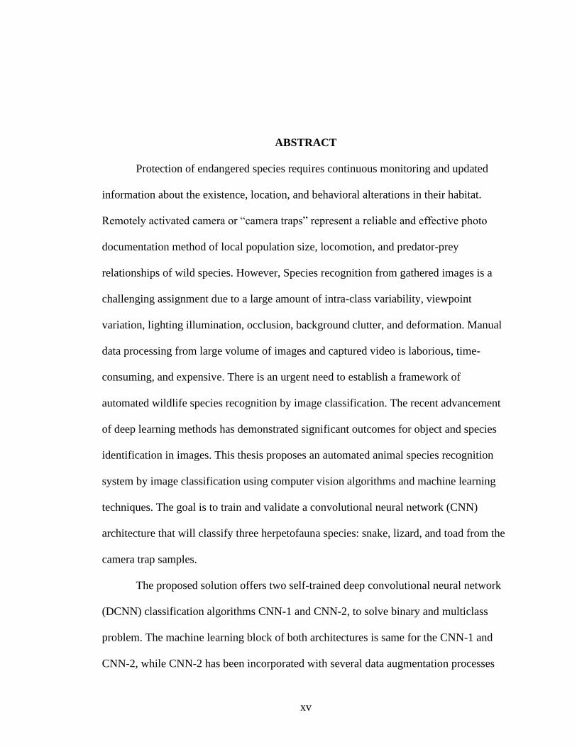
ABSTRACT
Protection of endangered species requires continuous monitoring and updated
information about the existence, location, and behavioral alterations in their habitat.
Remotely activated camera or “camera traps” represent a reliable and effective photo
documentation method of local population size, locomotion, and predator-prey
relationships of wild species. However, Species recognition from gathered images is a
challenging assignment due to a large amount of intra-class variability, viewpoint
variation, lighting illumination, occlusion, background clutter, and deformation. Manual
data processing from large volume of images and captured video is laborious, time-
consuming, and expensive. There is an urgent need to establish a framework of
automated wildlife species recognition by image classification. The recent advancement
of deep learning methods has demonstrated significant outcomes for object and species
identification in images. This thesis proposes an automated animal species recognition
system by image classification using computer vision algorithms and machine learning
techniques. The goal is to train and validate a convolutional neural network (CNN)
architecture that will classify three herpetofauna species: snake, lizard, and toad from the
camera trap samples.
The proposed solution offers two self-trained deep convolutional neural network
(DCNN) classification algorithms CNN-1 and CNN-2, to solve binary and multiclass
problem. The machine learning block of both architectures is same for the CNN-1 and
CNN-2, while CNN-2 has been incorporated with several data augmentation processes
xvi
such as rotation, zoom, flip, and shift to the existing samples during the training period.
Also, the impact of changing CNN parameters, optimizers, and regularization techniques
on classification accuracy is investigated in this study. The initial experiment implies
building a flexible binary and multiclass CNN architecture with labeled images
accumulated from several online sources. Once the baseline model is formulated and
tested with satisfactory accuracy, new camera trap imagery data is executed to the model
for recognition purpose. All three species have classified individually regarding
background samples to distinguish the presence of target species in a camera trap dataset.
The performance is evaluated based on the classification accuracy within their group
using two separate sets of validation and testing data. In the end, both models have tested
to predict the category of a new example to compare the models' generalization ability
with a challenging camera trap data.
1
1. INTRODUCTION
1.1 Motivation of The Research Work
Anthropogenic acquisition of natural resources and unplanned urbanization causes
substantial changes in geographical patterns and earth’s ecosystems. Due to massive
landscape fragmentation, the overall habitat structure changes, which harms wildlife
populations, habitat, and behavior. The two vertebrate classes, amphibia, and reptilia
collectively referred to as the herpetofauna [1], are among the globally endangered
species in conservation biology [2].
Since 1980, more than 120 species have been driven to extinction, and nearly one-
third of amphibian species are now considered threatened worldwide [2]. Twenty years
ago, researchers warned of habitat loss, and degradation as a primary threat to both
amphibian and reptile populations [1] [24]. The author in [1] also cited habitat
modification, introduced invasive species, disease, pollution, unsustainable use, and
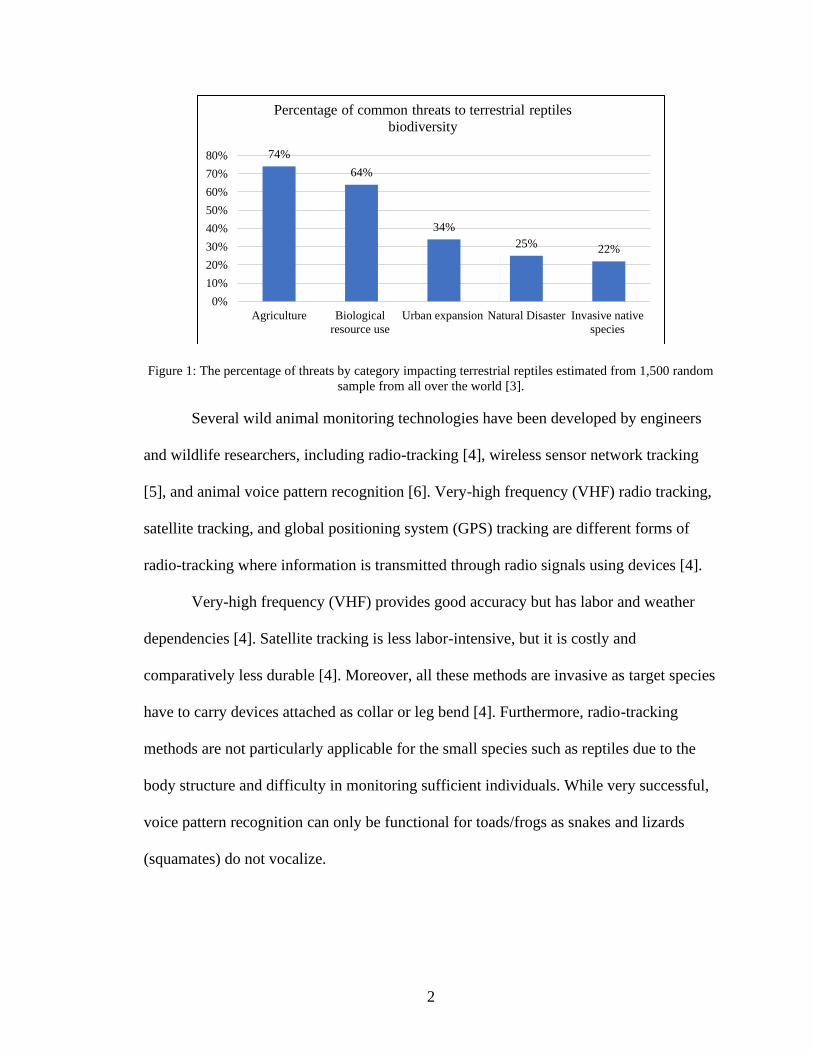
climate change as the six significant threats to reptile populations. In 2013, researchers
presented the first global estimation of the conservation status conducted on 1,500
random reptile samples from all over the world [3]. Their assessment shown in Figure 1
indicates that agriculture (74% of threatened species affected), biological resource use
(64%), urban expansion (34%), natural system alteration (25%), and invasive or
problematic native species (22%) played as threats to reptile biodiversity [3].
2
Figure 1: The percentage of threats by category impacting terrestrial reptiles estimated from 1,500 random
sample from all over the world [3].
Several wild animal monitoring technologies have been developed by engineers
and wildlife researchers, including radio-tracking [4], wireless sensor network tracking
[5], and animal voice pattern recognition [6]. Very-high frequency (VHF) radio tracking,
satellite tracking, and global positioning system (GPS) tracking are different forms of
radio-tracking where information is transmitted through radio signals using devices [4].
Very-high frequency (VHF) provides good accuracy but has labor and weather
dependencies [4]. Satellite tracking is less labor-intensive, but it is costly and
comparatively less durable [4]. Moreover, all these methods are invasive as target species
have to carry devices attached as collar or leg bend [4]. Furthermore, radio-tracking
methods are not particularly applicable for the small species such as reptiles due to the
body structure and difficulty in monitoring sufficient individuals. While very successful,
voice pattern recognition can only be functional for toads/frogs as snakes and lizards
(squamates) do not vocalize.
74%
64%
34%
25%22%
0%
10%
20%
30%
40%
50%
60%
70%
80%
Agriculture Biological
resource use
Urban expansion Natural Disaster Invasive native
species
Percentage of common threats to terrestrial reptiles
biodiversity
3
Data providing population size, dispersal, and the predator-prey relationships for
endangered species are required to understand their distribution, as well as the threat
processes’ distribution [3]. Wildlife researchers have experienced that visual information
provides definitive evidence of an animal’s presence and activity analysis against
environmental context [7]. The Department of Biology and The Ingram School of
Engineering at Texas State University, and Texas A&M University work together in a
“camera trap” project to identify species from images around the Texas. This thesis’s
outcome develops the basis of a mechanical structure to identify three broad groups of
herpetofauna, toads/frogs, lizards, and snakes in camera trap images using computer
vision and machine learning techniques.
1.2. Camera Traps in Wildlife Monitoring
Recent advancements in technology have allowed researchers to widespread the
adoption of minimally invasive camera trap monitoring system. Motion-triggered remote
cameras, commonly known as “camera traps,” are gaining popularity for reliable and
cost-effective applications [8]. Generally, camera traps are a static motion-sensor
framework attached with some structure or trees in the field, pointing towards animal
movement path [7]. The camera setup requires low labor engagement as it is quite simple
to deploy, flexible to operate, and easy to maintain in the field [8]. Most importantly, the
arrangement allows tracing the species secretly and continuously without disturbing their
surroundings [5]. This powerful tool captures a rich set of information about animal
appearance, actions, biometric features and provides critical evidence such as size can
indicate the age of the animal, or entry angle reveals the direction of the animal’s
movement [7]. Additionally, camera traps enable associated metadata, such as date, time,
4
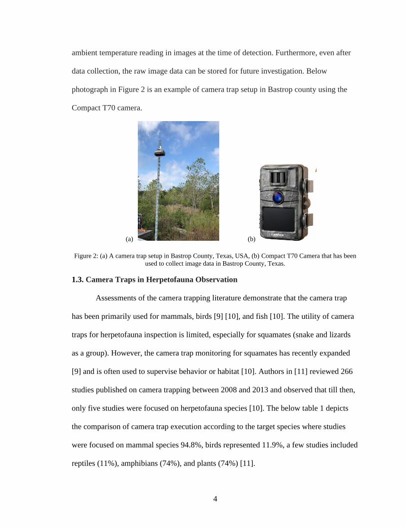
ambient temperature reading in images at the time of detection. Furthermore, even after
data collection, the raw image data can be stored for future investigation. Below
photograph in Figure 2 is an example of camera trap setup in Bastrop county using the
Compact T70 camera.
(a) (b)
Figure 2: (a) A camera trap setup in Bastrop County, Texas, USA, (b) Compact T70 Camera that has been
used to collect image data in Bastrop County, Texas.
1.3. Camera Traps in Herpetofauna Observation
Assessments of the camera trapping literature demonstrate that the camera trap
has been primarily used for mammals, birds [9] [10], and fish [10]. The utility of camera
traps for herpetofauna inspection is limited, especially for squamates (snake and lizards
as a group). However, the camera trap monitoring for squamates has recently expanded
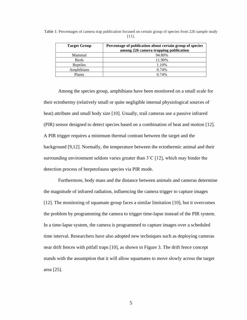
[9] and is often used to supervise behavior or habitat [10]. Authors in [11] reviewed 266
studies published on camera trapping between 2008 and 2013 and observed that till then,
only five studies were focused on herpetofauna species [10]. The below table 1 depicts
the comparison of camera trap execution according to the target species where studies
were focused on mammal species 94.8%, birds represented 11.9%, a few studies included
reptiles (11%), amphibians (74%), and plants (74%) [11].
5
Table 1: Percentages of camera trap publication focused on certain group of species from 226 sample study
[11].
Target Group Percentage of publication about certain group of species
among 226 camera trapping publication
Mammal 94.80%
Birds 11.90%
Reptiles 1.10%
Amphibians 0.74%
Plants 0.74%
Among the species group, amphibians have been monitored on a small scale for
their ectothermy (relatively small or quite negligible internal physiological sources of
heat) attribute and small body size [10]. Usually, trail cameras use a passive infrared
(PIR) sensor designed to detect species based on a combination of heat and motion [12].
A PIR trigger requires a minimum thermal contrast between the target and the
background [9,12]. Normally, the temperature between the ectothermic animal and their
surrounding environment seldom varies greater than 3˚C [12], which may hinder the
detection process of herpetofauna species via PIR mode.
Furthermore, body mass and the distance between animals and cameras determine
the magnitude of infrared radiation, influencing the camera trigger to capture images
[12]. The monitoring of squamate group faces a similar limitation [10], but it overcomes
the problem by programming the camera to trigger time-lapse instead of the PIR system.
In a time-lapse system, the camera is programmed to capture images over a scheduled
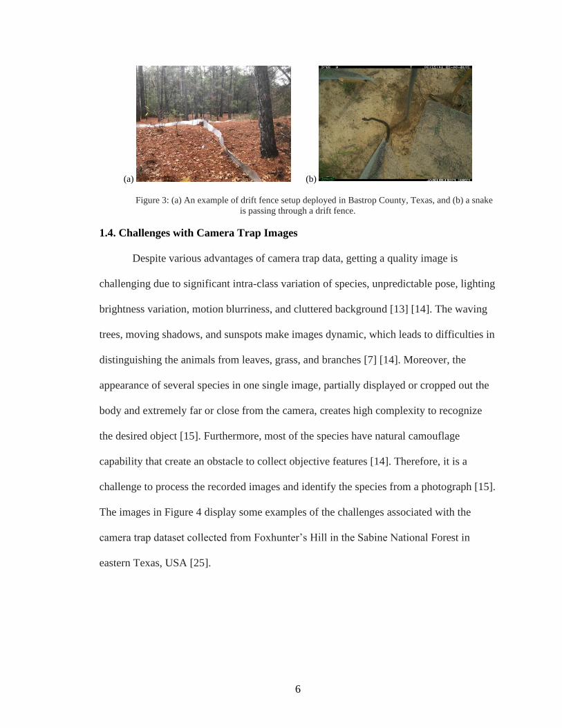
time interval. Researchers have also adopted new techniques such as deploying cameras
near drift fences with pitfall traps [10], as shown in Figure 3. The drift fence concept
stands with the assumption that it will allow squamates to move slowly across the target
area [25].
6
(a) (b)
Figure 3: (a) An example of drift fence setup deployed in Bastrop County, Texas, and (b) a snake
is passing through a drift fence.
1.4. Challenges with Camera Trap Images
Despite various advantages of camera trap data, getting a quality image is
challenging due to significant intra-class variation of species, unpredictable pose, lighting
brightness variation, motion blurriness, and cluttered background [13] [14]. The waving
trees, moving shadows, and sunspots make images dynamic, which leads to difficulties in
distinguishing the animals from leaves, grass, and branches [7] [14]. Moreover, the
appearance of several species in one single image, partially displayed or cropped out the
body and extremely far or close from the camera, creates high complexity to recognize
the desired object [15]. Furthermore, most of the species have natural camouflage
capability that create an obstacle to collect objective features [14]. Therefore, it is a
challenge to process the recorded images and identify the species from a photograph [15].
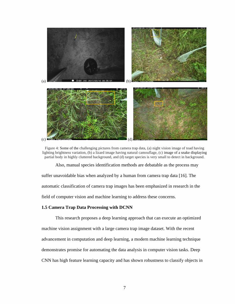
The images in Figure 4 display some examples of the challenges associated with the
camera trap dataset collected from Foxhunter’s Hill in the Sabine National Forest in
eastern Texas, USA [25].
7
(a) (b)
(c) (d)
Figure 4: Some of the challenging pictures from camera trap data, (a) night vision image of toad having
lighting brightness variation, (b) a lizard image having natural camouflage, (c) image of a snake displaying
partial body in highly cluttered background, and (d) target species is very small to detect in background.
Also, manual species identification methods are debatable as the process may
suffer unavoidable bias when analyzed by a human from camera trap data [16]. The
automatic classification of camera trap images has been emphasized in research in the
field of computer vision and machine learning to address these concerns.
1.5 Camera Trap Data Processing with DCNN
This research proposes a deep learning approach that can execute an optimized
machine vision assignment with a large camera trap image dataset. With the recent
advancement in computation and deep learning, a modern machine learning technique
demonstrates promise for automating the data analysis in computer vision tasks. Deep
CNN has high feature learning capacity and has shown robustness to classify objects in

8
challenging images. This method offers tremendous opportunities for automated species
identification from a high volume of biological image data.
The aim of the thesis is to build a structure that will recognize and classify
frogs/toads, snakes, and lizards from a given set of a large camera trap dataset collected
from different locations within Texas. Building a machine learning model involves
following steps, as shown in Figure 5.
Figure 5: An overall workflow diagram of the research work having four major steps of image
classification procedure using DCNN algorithm.
1.6 Thesis Outline
This thesis is organized as follows. Chapter II describes about the previous
initiatives taken by Texas State University to protect endangered species, a little
introduction about citizen science projects and ImageNet challenges. In Chapter III, a
detailed literature review based on the previous work related to species classification with
DCNN has been highlighted. In Chapter IV, thesis design approach and classification
pipeline have been explained in short. Chapter V talks about data accusation, and
characteristic of both datasets: online and camera trap with some example images.
Chapter VI entails all about DCNN building block and architecture. Chapter VII is the
methodology chapter of the research work that describes data preprocessing, data
partitioning and the model architectures. Chapter VIII discusses the experiment and
results analysis. Finally, Chapter IX summarizes the overall research contributions, and
the possible future research.
9
2. BACKGROUND
2.1 Camera Trap Project Initialization by Texas State University
An array of research conducted by the Department of Biology of Texas State
University pursues the inventory of the relative density, distribution of herpetofauna
community, and herpetological assemblage using standard sampling technique within
Texas [19]. The researchers of the Biology department have actively performed several
investigations to understand the motive behind herpetofauna population decline; such as
Allee effects of a correlation between population density and the mean individual fitness
in the conservation of endangered anurans, [20] or the impact of natural calamities such
as drought and wildfire on herpetofauna species [21]. In the past few years, they are
experimenting with ‘Toad Phone’ development projects in collaboration with the Ingram
School of Engineering. That project aims to trace the Houston toad (Bufo houstonensis)
breeding activity using Automated Recording Devices (ARD’s) that store environmental
information and send notifications in near real-time [22][23]. However, only male
amphibians chorus. Therefore, image data collected by the camera traps presents new
diagnostic opportunities to detect and monitor species, including females of the
amphibians and other herpetofauna.
The camera trap data has been utilized since 2004 to complement the amphibian
and other species detection process. In 2019, fourteen cameras were attached near drift
fence arrays in Bastrop County, Texas, where data was collected five times from
September to December. Each camera captured roughly 10,000 images stored in a 32 GB
SD card resulting in millions of images. Though these cameras provide a large volume of
serialized data, less than 1% of the images are likely to have valuable information such as
10
species’ presence, and the remaining images only contain background environmental
information. Among those species’ images, it can be expected that about one-tenth of the
images might have any of the three target groups of interest. Due to the unavailability of
computation framework, data had to be analyzed manually. Distinguishing empty frames
and target species from a vast dataset are still done by human reviewers, which is a
monotonous and time-consuming task. For the assessment of the extensive database, an
automatic system should be established, allowing researchers to focus only on essential
analyses and evaluation of animal detections.
A reliable object recognition framework is needed to provide substantial time
saving procedures to manage large image datasets. The modern machine learning
approach is gradually paving into the field of species identification. The theory and the
mathematical foundations for neural network were laid several decades ago [17]. The
availability of massive datasets, advancement of raw compute power, and efficient
parallel hardware have contributed to the rise of machine learning applications [17] [18].
The potentiality of computer vision technology and deep neural network to classify
images has provided an improved wildlife monitoring system reducing classification time
and manual effort.
2.2 Citizen Science Projects
Researchers seek data to evaluate the biodiversity crisis and to understand the
impacts of human actions or natural environmental changes to create effective resource
management decisions and stewardship of wildlife species. In recent years, ecologists,
biologists, engineers, researchers, and volunteers collaborate in citizen science (also
known as crowd-sourced) projects to support wildlife monitoring and research. For
11
example, ‘Zooniverse’ is the largest people-powered research community where millions
of volunteers assist professional researchers in producing reliable and accurate data by
labeling, and analyzing images [27]. This online platform provides standard guidelines
and annotation tools to the researcher to extract information more quickly and accurately
[26]. Until October 2019, Zooniverse has hosted 111 camera trap projects, producing
millions of images of wild species worldwide, and citizen scientists are analyzing data
remotely via web-based image classification systems [27]. The first camera trap project
Snapshot Serengeti (SS) contains images of 48 animal species acquired from 225 cameras
placed in Serengeti National Park, Tanzania [26].
Traditionally, species classification is being conducted by morphological
diagnostic process provided by taxonomic studies specialists which requires skills
obtained through extensive experience [28]. However, the researchers realized the need
for automated and accurate identification methods over time [28]. The modern artificial
intelligence systems are providing an alternative tool for identification tasks [28]. A
couple of studies have been done with a crowdsourced camera trap dataset applying deep
neural network in the last few years. The outcome portrays the ability to extract valuable
knowledge from camera trap images using deep neural networks (DNNs). Some of the
studies regarding the camera trap citizen science project will be highlighted in the
literature review chapter
2.3 Pre-trained Deep Learning Models
In the machine vision research field, an organized large-scale image database is
necessary with the facility of web-based data storage. The “ImageNet” project facilitates
millions of labeled and categorized images for the computer vision and deep learning
12
communities [17]. This platform has recently hosted the ImageNet Large Scale Visual
Recognition Challenge (ILSVRC) annual competition from 2010 to 2017. The main
challenges were image classification, single-object localization, and object detection
using 1,000 categories from the ImageNet dataset [17]. The accuracy of the winning
ILSVRC has improved significantly every year, showcasing the progress in terms of
state-of-the-art performance. The deep convolutional neural networks (DCNNs)
architectures achieved tremendous success overtime in object classification, object
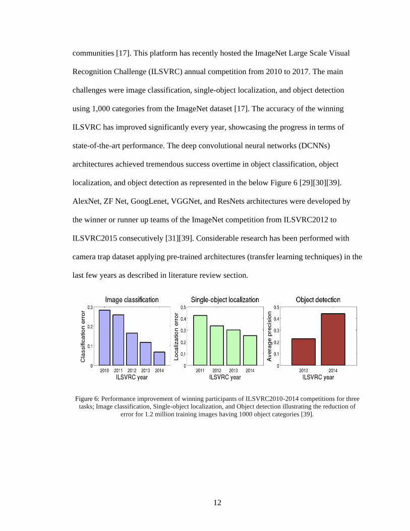
localization, and object detection as represented in the below Figure 6 [29][30][39].
AlexNet, ZF Net, GoogLenet, VGGNet, and ResNets architectures were developed by
the winner or runner up teams of the ImageNet competition from ILSVRC2012 to
ILSVRC2015 consecutively [31][39]. Considerable research has been performed with
camera trap dataset applying pre-trained architectures (transfer learning techniques) in the
last few years as described in literature review section.
Figure 6: Performance improvement of winning participants of ILSVRC2010-2014 competitions for three
tasks; Image classification, Single-object localization, and Object detection illustrating the reduction of
error for 1.2 million training images having 1000 object categories [39].

13
3. LITERATURE REVIEW
This chapter provides a literature survey of research work that focuses on
identifying species using machine vision techniques and deep learning technique
published in various conference and journal papers. The majority of the research work on
plant or animal species recognition have been performed with image samples taken by
digital cameras in labs or natural habitats. However, numerous species recognition
experiments with camera trap image have been conducted recently, mostly for mammals
and bird group, and more research is getting published with gradual improvement over
time. In the subsequent paragraphs, some of the academic research for camera trap image
identification using the different techniques are discussed. Also, some of the experiments
with target species using online data have been considered for review.
3.1 Species Identification Using Feature Extractor and Classifier
Most of the camera-based wildlife experiments are done to identify individual
animals with unique coat patterns such as spots, stripes [32], shape, and texture [33]. In
past years, different algorithms were used as feature extractors or image descriptors to
obtain features such as shape, texture, color from input images, and quantify the
individual aspect with statistical analysis [33, 16]. The traditional image classification
process consists of a hand-defined feature extraction algorithm, followed by a machine
learning classifier [33]. On the other hand, the deep learning networks approach
automatically learns features from input images in the training process, eliminating rules
and algorithms to extract features [33].
Studies suggest that ten years ago, bag-of-features (BoF) was the utmost popular
image categorization task [34, 35]. Authors in [34, 35] classified BOF along with spatial
14
pyramid matching (SPM) as a state-of-the-art image classification system. In 2013, the
first complete analysis with a camera trap dataset was done by authors in [32] using the
Scale-Invariant Feature Transformation (SIFT) algorithm in combination with a Support
Vector Machine (SVM) to classify species. The researchers collected seven thousand
camera trap images of 18 species from two different field sites for the experiment that
achieved an average classification accuracy of 82%. The authors applied improved sparse
coding spatial pyramid matching (ScSPM), SIFT descriptor, and cell-structured local
binary patterns (cLBP). Feature generation was done by weighted sparse coding and max
pooling using multi-scale pyramid kernel, and classification of the images was done by
linear support vector machine (SVM) algorithm.
3.2. Camera Trap Dataset with Deep Neural Network
In 2014, the first CNN application can be observed in [5] where the authors
presented a comparison of results between two-image classification algorithms, Bag of
Visual Words (BOW) and DCNN. The dataset contains 20 species having 14,346 training
images and 9,530 testing images. In the BOW method, a 128-dimensional Scale-invariant
feature transform (SIFT) algorithm was used to extract the feature, and linear SVM was
used as a classifier. On the other hand, three convolutional layers and three max-pooling
layers were implemented in the DCNN method with a data augmentation step in the
training stage. With a very challenging noisy dataset, DCCN showed promising results
with 38.315% accuracy, where BOW’s accuracy was 33.507%.
The ILSVRC DCNN model architecture from ImageNet competition has provided
a dominant win over traditional algorithms [5]. Moreover, the publicly available citizen
science dataset has opened an opportunity to do more research for camera trap data using
15
DCNN. In 2016, eight variations of CNN frameworks AlexNet, VGGNet, GoogLenet,
and ResNets were used to identify 26 classes of animal species from highly unbalanced
Snapshot Serengeti dataset [15]. The number of layers of the mentioned CNN
architectures varied from eight (AlexNet) to 152 (ResNet-152), where ResNet-101
architecture achieved the best performance [15].
In the research found in [36], the authors also experimented with nine
independent architectures, including AlexNet, NiN, VGG, GoogLeNet, and numerous
variations of ResNets with 48 species in the 3.2-million-images of Snapshot Serengeti
dataset. Also, to detect species, authors have trained the model to identify further
attributes; presence, counting, and behaviors (the presence of young). Similar work has
been found in [29], where authors reviewed different CNN architecture (AlexNet,
VGGNet, and ResNets) in automatic identification for two subsequent tasks: (a) filter
images containing animal from a set of Wildlife Spotter project dataset, (b) then
classifying species automatically. The model achieved more than 96% in recognizing
animals in images and close to 90% in identifying three common animals (bird, rat,
bandicoot).
In 2018, authors in [16] compared the performance of two algorithms Faster
Region-Convolutional Neural Network and You-Only-Look-Once v2.0, to identify and
quantify animal species on two different datasets; Reconyx Camera Trap and the self-
labeled Gold Standard Snapshot Serengeti data sets. The findings demonstrated that
YOLO has speed advantages and can be used in real-time performance, whereas Faster
R-CNN represented promising results with average accuracy of 76.7% and 93.0%,
respectively.
16
Authors in [37] trained 3,367,383 camera trap images from five states across the
United States with convolutional neural networks with the ResNet-18 architecture
providing 98%, which is the highest accuracy to date. Recently authors in [38] have
trained 8,368 images having six categories: badger, bird, cat, fox, rat, and rabbit with two
different networks; a self‐trained framework (CNN‐1) and pre-trained model AlexNet
(CNN-2) where CNN-2 outperformed CNN-1.
3.3 Target Species Recognition Using Deep Neural Network
Most Recently, few recognition experiments of target species (snake and lizard)
have been conducted using online dataset applying deep learning techniques. So far, no
work has been found focusing on toad/frog detection from images using deep learning
technique.
In the research found in [14], lizard was detected and counted from drone images
applying pixel-wise image segmentation deep learning approach “U-Net”. The author had
to train the model with 600 online datasets as the captured images by drone did not
provide sufficient sample to do the experiment. The highest validation accuracy the
model achieved is 98.63% using a batch normalization in atrous blocks of the U-Net
model.
In 2018, authors in [76] classified five venomous snake species in Indonesia with
415 samples. The authors performed the experiment with three different self-trained CNN
models; shallow, medium, and deep CNN architectures by changing filter size and by
adding more layers. With the five-fold cross-validation process, the medium architecture
offered the best performance with an average accuracy of 82%.
17
For the work in [77], experiments have been performed a real-time identification
of snakes of the Galápagos Islands, Ecuador by applying object detection and image
classification approach. Four region-based convolutional neural network (R-CNN)
architectures have been tested for object detection: Inception V2, ResNet, MobileNet, and
VGG16. The experiment studied 247 snake images of 9 species where ResNet achieved
the best classification accuracy of 75%, Inception V2, and VGG16 scored 70% for the
given dataset.
In 2020, the LifeCLEF research platform arranged a four round SnakeCLEF 2020
challenge focusing on the automated snake identification from large online dataset [78].
The task of this experiment was to distinguish 783 different snake species from 245,185
training and 14,029 validation samples [78]. As an object detection method, the
researchers in paper [78] used Mask Region-based Convolutional Neural Network (Mask
R-CNN) with EfficientNets for classification and associated location information of the
samples. The initial result with the best model achieved a macro-averaging F1-score of
0.404 that has been improved afterword with a macro-averaging F1-score of 0.594.
3.4 Thesis Contributions
After research, it can state that this is the first attempt to recognize herpetofauna,
especially snake, frog/toad, with a DCNN approach from camera trap images. This
project intends to work with different CNN architectures with both online datasets
(collected from the internet) and a camera trap dataset (collected from the field). Previous
experiments, assessment, and analysis of the works suggest that DCNN is a suitable
technique to extract valuable knowledge from images.
18
The goals of this study are -
(a) To present an automated framework of photo identification for animal species
by constructing, testing, refining an image classification algorithm for both sample sets;
online dataset and camera trap dataset.
(b) To investigate several image pre-processing solutions to mitigate challenges
in the dataset by applying image augmentation techniques.
19
4. THESIS IMPLEMENTATION STRATEGY
The ultimate thesis’s objective is to develop a computer vision and machine
learning solution that will classify all three species (snakes, lizards, and frogs)
individually and separately in different pictures. In image classification, the core task is
to assign a label to an image from a predefined set of possible categories. The workflow
of methodology starts with collecting samples, preprocessing datasets, training a CNN
model architecture, and evaluating the classifier on a withheld set of test images. Figure 7
shows an overview process of the proposed design approach.
Figure 7: An image classification pipeline using DCNN techniques representing four main steps.
Two different CNN architecture referred as CNN-1 and CNN-2 have been
constructed and later have been trained, evaluated, and compared under the given
datasets. The fundamental building block of the DCNN framework, which is layers,
parameters are the same for both models. The only difference between the two models is
applying several data augmentation techniques in the second model to artificially enlarge
the size of a training dataset by creating modified versions of images. The basic idea is to
20
compare the generalization ability of two models for a new set of the testing dataset in the
evaluation period. An elaborate explanation of sample augmentation methods has been
described in Chapter VII. The main building block of the two models is picturized in
Figure 8.
Figure 8: Building blocks of CNN-1 and CNN-2 where CNN-2 have an added augmentation step for
the training data with different transformation techniques.
For the convenience of the experiment, the model implementation is divided into
two phases as defined below.
Phase one: The first phase comprises developing a baseline model from scratch to
classify species from images, not necessarily camera trap data. This phase applies the
dataset of 13,500 target species samples collected from various web database sources. The
first phase is a primary learning stage where two basic CNN architecture has formed with
several layers and combination of hyperparameters. Both the models have been trained
with the assembled dataset and were evaluated by the ability to separate species into their
category. Through several analysis and performance testing, gradual improvements have
been made in the model construction over time.
21
The model design was formed into several techniques to accomplish the
identification process in an efficient way.
(a) combinations of any two species: Both architectures have been designed to solve
a classical binary classification problem where the prediction result was measured for any
two classes, such as snake-lizard or toad-snake. This task involves training, validation,
and testing photos containing only two animal species at a time.
(b) combination of all three species: This structure considers a multiclass recognition
formation with all three species. The algorithm has trained with single labeled three
category images altogether, and the output provides classification accuracy for three
species. The models have experienced necessary changes, especially in hyperparameters
such as loss function, learning rate, and other network parameters.
Phase two: In the second phase, both the models were equipped with imagery camera
trap data. Here, the previous models were used to train new data where several
hyperparameter adjustments have been made according to the camera trap image
identification process. Similar to phase one; first the execution was tested with the
combinations of any two species, and later each of the models was performed for all three
species.
For each technique, every architecture will be customized to show a high
prediction probability for the test dataset. The network architecture needed to tune with
several hyperparameters such as learning rate, activation fiction, epoch size, batch size,
number of units, and other parameters to obtain optimal performance. The final model was
chosen carefully considering the highest classification accuracy for all their species
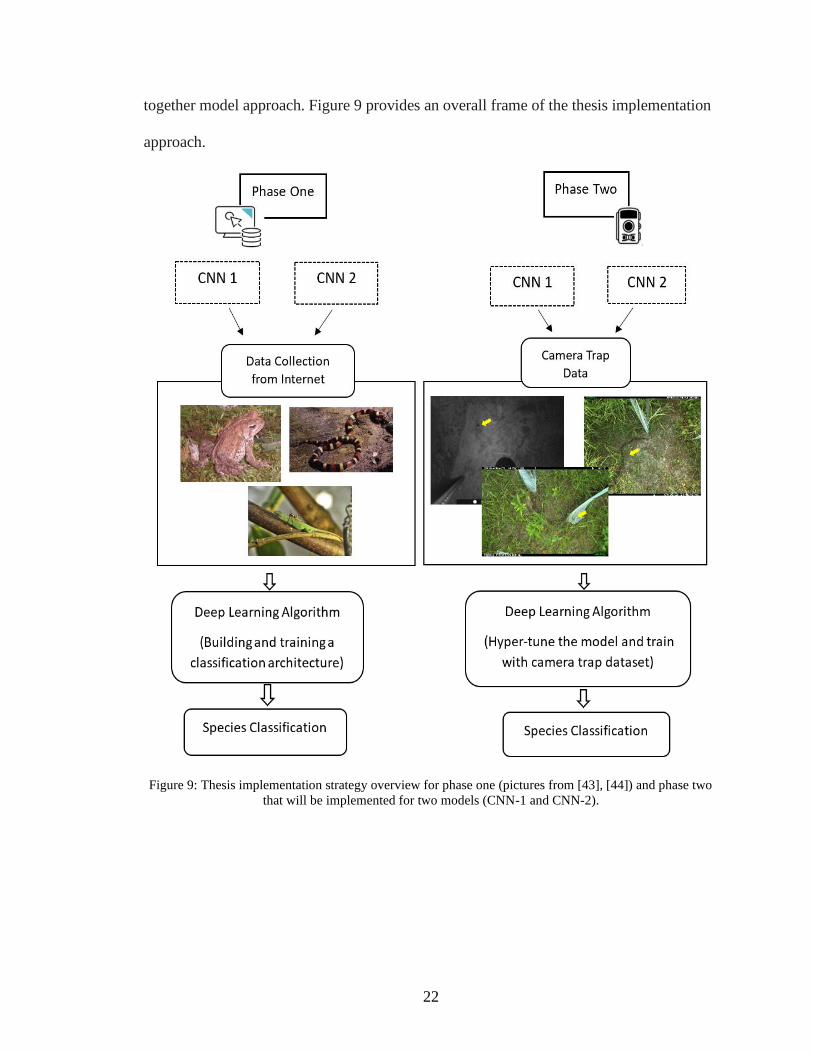
22
together model approach. Figure 9 provides an overall frame of the thesis implementation
approach.
Figure 9: Thesis implementation strategy overview for phase one (pictures from [43], [44]) and phase two
that will be implemented for two models (CNN-1 and CNN-2).
23
5. DATASET
For image classification problem, the dataset refers to a collection of images
where each image is a data point [33]. Machine learning algorithms are heavily
dependent on the size of dataset [40]. Elaborately, the algorithm's learning ability is
determined by the amount of quality information that holds the key factor of an image
[33]. A useful dataset is essential to prepare a CNN model to perform the classification
task when unobserved data is given. In this project, most of the research time is allocated
to accumulate and preprocess datasets. The subsequent subsections describe data
gathering process, sources, characteristics, and changes of two kinds of dataset: online
dataset (phase one) and camera trap dataset (phase two).
5.1 Online Dataset (Phase One)
5.1.1 Data Accumulation
For this project's initial experiment, 13,500 photographs of snake, lizard, and
toad/frog were collected from various online sources. Most of the images have been
collected from standard benchmark datasets such as Caltech, CalPhotos, and Open
Images. In contrast, some photos have been collected from image classification challenge
[67] and the online photo archive [44], [75]. “CalPhotos,” is an online image database
specialized in plants, animals, and natural history [41]. This database is a project of
Berkeley Natural History Museums and the University of California, where images are
stored with descriptive information about scientific and common names, locations, dates,
and contributor’s information [41].
Open Image is one of the largest online databases released by google dedicated to
image classification and object detection. The web portal contains 600 object categories
24
of images annotated with labels, object bounding boxes, object segmentation masks, and
localized narratives [42]. Around 2,000 snake, toad and lizard images have been
downloaded from Open Images V6 following their instructions. Also, 500 snake and frog
image data were stored from Caltech, a standard public dataset [43].
Nearly 1,000 images were accumulated from the Bing Image Search API that
facilitates custom search images provided by the Microsoft Bing web portal [45].
Another 1,000 images have been gathered from a crowdsourced online website Unsplash
and Pixabay [44], [75]. However, acquired images from Microsoft Bing needed manual
examination to clean unwanted samples of target species such as animation, graphics, or
sketch.
5.1.2 Specifications of Online Dataset
The downloaded dataset portrays that most of the subject species are free-living
animals where images are captured in an open environment. Some of the pictures are
captured in laboratory settings. In phase one, target animal species have been chosen with
numerous variations of color, size, and background to let the model learn the features
properly. The animal body was visible about 20-80% of the whole pixelated area of an
image. However, those images suffer from dynamic object position, light illumination,
occlusion, complex animal poses, and significant intra-class variation within their group.
Below samples in Figure 10, 11, 12, 13 show some of the attributes that have been
considered while building the CNN model.
25
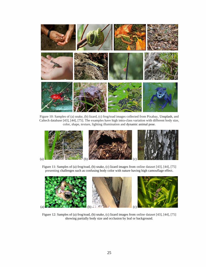
Figure 10: Samples of (a) snake, (b) lizard, (c) frog/toad images collected from Pixabay, Unsplash, and
Caltech database [43], [44], [75]. The examples have high intra-class variation with different body size,
color, shape, texture, lighting illumination and dynamic animal pose.
(a) (b) (c)
Figure 11: Samples of (a) frog/toad, (b) snake, (c) lizard images from online dataset [43], [44], [75]
presenting challenges such as confusing body color with nature having high camouflage effect.
(a) (b) (c)
Figure 12: Samples of (a) frog/toad, (b) snake, (c) lizard images from online dataset [43], [44], [75]
showing partially body size and occlusion by leaf or background.
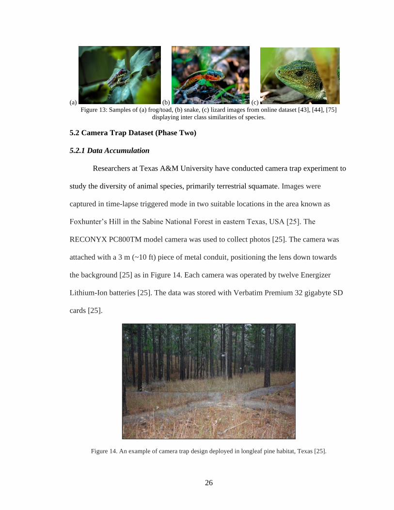
26
(a) (b) (c)
Figure 13: Samples of (a) frog/toad, (b) snake, (c) lizard images from online dataset [43], [44], [75]
displaying inter class similarities of species.
5.2 Camera Trap Dataset (Phase Two)
5.2.1 Data Accumulation
Researchers at Texas A&M University have conducted camera trap experiment to
study the diversity of animal species, primarily terrestrial squamate. Images were
captured in time-lapse triggered mode in two suitable locations in the area known as
Foxhunter’s Hill in the Sabine National Forest in eastern Texas, USA [25]. The
RECONYX PC800TM model camera was used to collect photos [25]. The camera was
attached with a 3 m (~10 ft) piece of metal conduit, positioning the lens down towards
the background [25] as in Figure 14. Each camera was operated by twelve Energizer
Lithium-Ion batteries [25]. The data was stored with Verbatim Premium 32 gigabyte SD
cards [25].
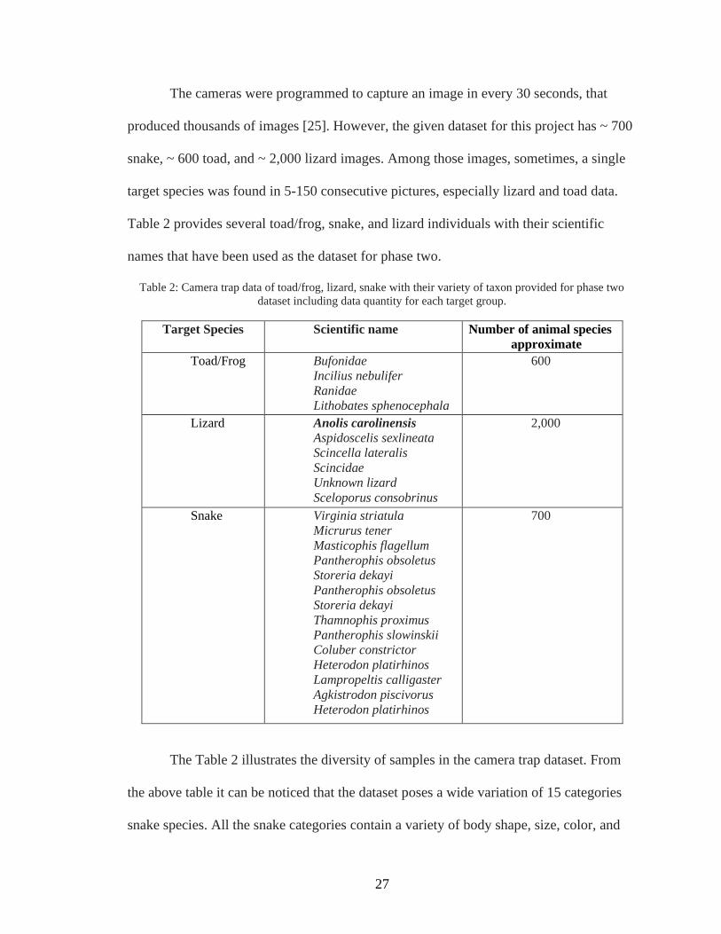
Figure 14. An example of camera trap design deployed in longleaf pine habitat, Texas [25].
27
The cameras were programmed to capture an image in every 30 seconds, that
produced thousands of images [25]. However, the given dataset for this project has ~ 700
snake, ~ 600 toad, and ~ 2,000 lizard images. Among those images, sometimes, a single
target species was found in 5-150 consecutive pictures, especially lizard and toad data.
Table 2 provides several toad/frog, snake, and lizard individuals with their scientific
names that have been used as the dataset for phase two.
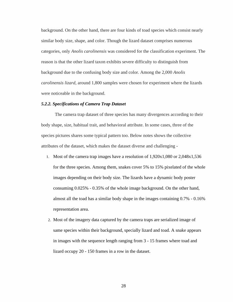
Table 2: Camera trap data of toad/frog, lizard, snake with their variety of taxon provided for phase two
dataset including data quantity for each target group.
Target Species Scientific name Number of animal species
approximate
Toad/Frog Bufonidae
Incilius nebulifer
Ranidae
Lithobates sphenocephala
600
Lizard Anolis carolinensis
Aspidoscelis sexlineata
Scincella lateralis
Scincidae
Unknown lizard
Sceloporus consobrinus
2,000
Snake Virginia striatula
Micrurus tener
Masticophis flagellum
Pantherophis obsoletus
Storeria dekayi
Pantherophis obsoletus
Storeria dekayi
Thamnophis proximus
Pantherophis slowinskii
Coluber constrictor
Heterodon platirhinos
Lampropeltis calligaster
Agkistrodon piscivorus
Heterodon platirhinos
700
The Table 2 illustrates the diversity of samples in the camera trap dataset. From
the above table it can be noticed that the dataset poses a wide variation of 15 categories
snake species. All the snake categories contain a variety of body shape, size, color, and
28
background. On the other hand, there are four kinds of toad species which consist nearly
similar body size, shape, and color. Though the lizard dataset comprises numerous
categories, only Anolis carolinensis was considered for the classification experiment. The
reason is that the other lizard taxon exhibits severe difficulty to distinguish from
background due to the confusing body size and color. Among the 2,000 Anolis
carolinensis lizard, around 1,800 samples were chosen for experiment where the lizards
were noticeable in the background.
5.2.2. Specifications of Camera Trap Dataset
The camera trap dataset of three species has many divergences according to their
body shape, size, habitual trait, and behavioral attribute. In some cases, three of the
species pictures shares some typical pattern too. Below notes shows the collective
attributes of the dataset, which makes the dataset diverse and challenging -
1. Most of the camera trap images have a resolution of 1,920x1,080 or 2,048x1,536
for the three species. Among them, snakes cover 5% to 15% pixelated of the whole
images depending on their body size. The lizards have a dynamic body poster
consuming 0.025% - 0.35% of the whole image background. On the other hand,
almost all the toad has a similar body shape in the images containing 0.7% - 0.16%
representation area.
2. Most of the imagery data captured by the camera traps are serialized image of
same species within their background, specially lizard and toad. A snake appears
in images with the sequence length ranging from 3 - 15 frames where toad and
lizard occupy 20 - 150 frames in a row in the dataset.
29
3. Day images have more alteration in the background due to changing brightness
illumination over the day. Night vision pictures provide an advantage of less
cluttered background as IR mode produces grayscale images offering less lighting
intensity variation.
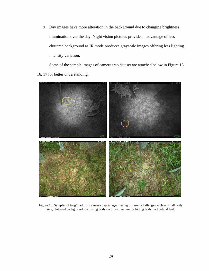
Some of the sample images of camera trap dataset are attached below in Figure 15,
16, 17 for better understanding.
Figure 15: Samples of frog/toad from camera trap images having different challenges such as small body
size, cluttered background, confusing body color with nature, or hiding body part behind leaf.
30
Figure 16: Samples of snake from camera trap images dataset having different body size, confusing body
color with nature, or hiding body part behind leaf.
Figure 17: Samples of lizard from camera trap images having different challenges such as small body size,
cluttered background, confusing body color with nature, or hiding body part behind leaf
31
6. DEEP LEARNING
6.1 Artificial Neural Network
Artificial neural network (ANN) is a supervised learning technique built with
many of artificial unit components named “neurons.” Neurons are organized in
interconnected layers where each neuron can make simple decisions and transfer those
decisions to other neurons. The architecture uses different layers to learn aspects,
recognize patterns, and analyze different factors similar to the human neural system [46].
Machine learning (ML) algorithms, neural networks, and deep learning fall into the
domain of Artificial intelligence (AI) as shown in the Figure 18.
Figure 18. A Venn diagram describing relationship between artificial intelligence, machine learning, neural
networks, and deep learning.
Artificial intelligence (AI): AI is a broader concept which builds intelligent programs
and machines that can creatively solve problems [46].
Machine learning (ML): ML is a subfield of AI providing a system to learn and
improve automatically from experience through an explicit program with minimal human
interaction [46]. The algorithm can understand the relationship between input-output data
and predict the value or the class when a new data point is given [47]. In ML, a neural
32
network or deep neural network is a widely used technique to handle large parameter
problems in a non-linear approach.
Neural Networks: Neural networks are a subfield of machine learning that works
excellent where the volume of data and the number of variables or diversity of the data is
massive [48]. The basic idea of a neural network is that it can depict associations and
discover consistencies within a set of patterns from data.
Deep Learning: Deep learning is nothing but a richer structure of a neural network.
Deep learning is considered as the new state of the art in the territory of artificial
intelligence [47]. These are multi-level structures that extract detailed information from
input data such as patterns, speech, images, and other applications.
There are a few reasons behind the growth of ANNs over other ML techniques on
substantial and complex problems [50]. A tremendous improvement can be noticed in the
device capabilities such as memory capacity, power consumption, image sensor
resolution, and optics [52]. Since the 1990’s, computing power surged incredibly, making
it feasible to train large neural networks in a reasonable amount of time [50]. Moreover,
powerful GPU cards are available due to the progression of the gaming industry [50].
Deep neural networks can drastically reduce model execution time by taking advantage
of GPU for computation. Furthermore, the data availability in huge quantities adds an
impact to train a neural network. All the factors together lead researchers to focus more
on DNN, which eventually improves the training algorithm over time. Thus, the deep
learning performance has been upgraded, providing cost-efficiency and speed
acceleration of vision-based applications [50].
33
The structure of neural networks is simulated by the information processing
patterns of the human brain [33,49]. A typical brain contains millions of neurons (basic
computational unit) connected with synapses. A neuron receives input signals from
numerous dendrites and produces output signals towards the axon. The end of axon
branches is out to connect with dendrites of other neurons via synapses. The neuron only
triggers and sends a spike through the axon when the combination of input signals from
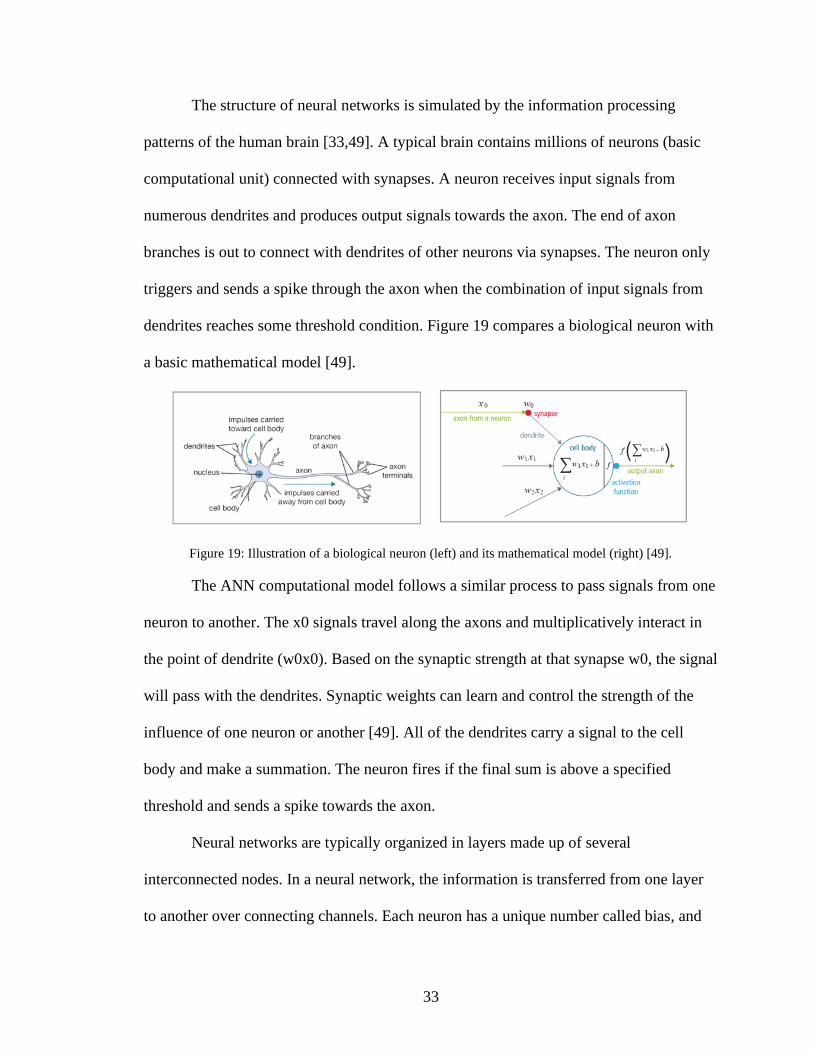
dendrites reaches some threshold condition. Figure 19 compares a biological neuron with
a basic mathematical model [49].
Figure 19: Illustration of a biological neuron (left) and its mathematical model (right) [49].
The ANN computational model follows a similar process to pass signals from one
neuron to another. The x0 signals travel along the axons and multiplicatively interact in
the point of dendrite (w0x0). Based on the synaptic strength at that synapse w0, the signal
will pass with the dendrites. Synaptic weights can learn and control the strength of the
influence of one neuron or another [49]. All of the dendrites carry a signal to the cell
body and make a summation. The neuron fires if the final sum is above a specified
threshold and sends a spike towards the axon.
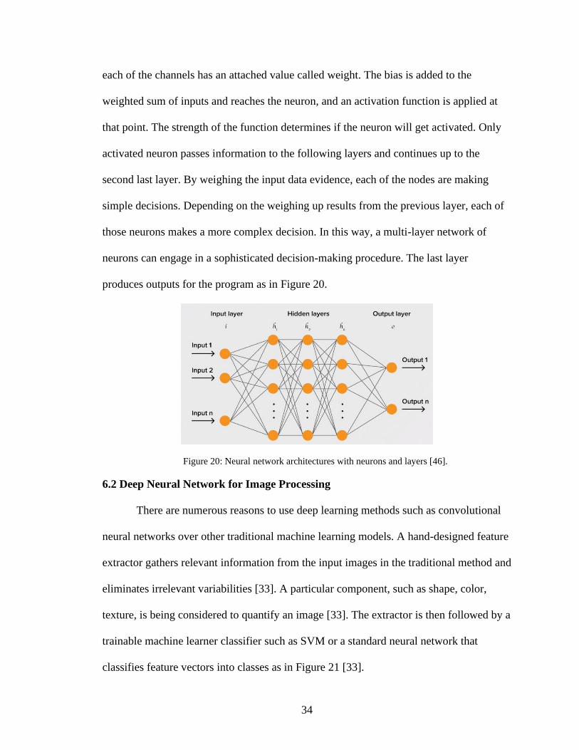
Neural networks are typically organized in layers made up of several
interconnected nodes. In a neural network, the information is transferred from one layer
to another over connecting channels. Each neuron has a unique number called bias, and
34
each of the channels has an attached value called weight. The bias is added to the
weighted sum of inputs and reaches the neuron, and an activation function is applied at
that point. The strength of the function determines if the neuron will get activated. Only
activated neuron passes information to the following layers and continues up to the
second last layer. By weighing the input data evidence, each of the nodes are making
simple decisions. Depending on the weighing up results from the previous layer, each of
those neurons makes a more complex decision. In this way, a multi-layer network of
neurons can engage in a sophisticated decision-making procedure. The last layer
produces outputs for the program as in Figure 20.
Figure 20: Neural network architectures with neurons and layers [46].
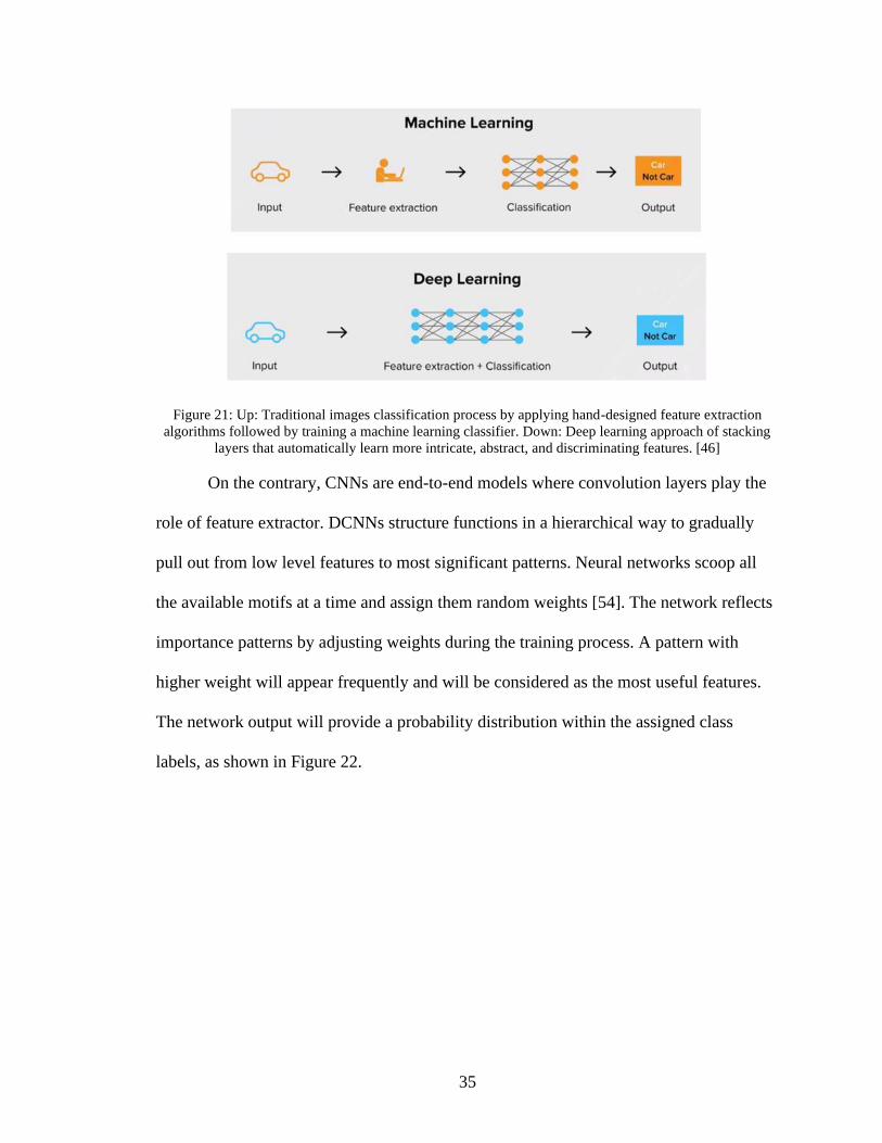
6.2 Deep Neural Network for Image Processing
There are numerous reasons to use deep learning methods such as convolutional
neural networks over other traditional machine learning models. A hand-designed feature
extractor gathers relevant information from the input images in the traditional method and
eliminates irrelevant variabilities [33]. A particular component, such as shape, color,
texture, is being considered to quantify an image [33]. The extractor is then followed by a
trainable machine learner classifier such as SVM or a standard neural network that
classifies feature vectors into classes as in Figure 21 [33].
35
Figure 21: Up: Traditional images classification process by applying hand-designed feature extraction
algorithms followed by training a machine learning classifier. Down: Deep learning approach of stacking
layers that automatically learn more intricate, abstract, and discriminating features. [46]
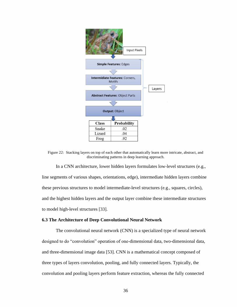
On the contrary, CNNs are end-to-end models where convolution layers play the
role of feature extractor. DCNNs structure functions in a hierarchical way to gradually
pull out from low level features to most significant patterns. Neural networks scoop all
the available motifs at a time and assign them random weights [54]. The network reflects
importance patterns by adjusting weights during the training process. A pattern with
higher weight will appear frequently and will be considered as the most useful features.
The network output will provide a probability distribution within the assigned class
labels, as shown in Figure 22.
36
Figure 22: Stacking layers on top of each other that automatically learn more intricate, abstract, and
discriminating patterns in deep learning approach.
In a CNN architecture, lower hidden layers formulates low-level structures (e.g.,
line segments of various shapes, orientations, edge), intermediate hidden layers combine
these previous structures to model intermediate-level structures (e.g., squares, circles),
and the highest hidden layers and the output layer combine these intermediate structures
to model high-level structures [33].
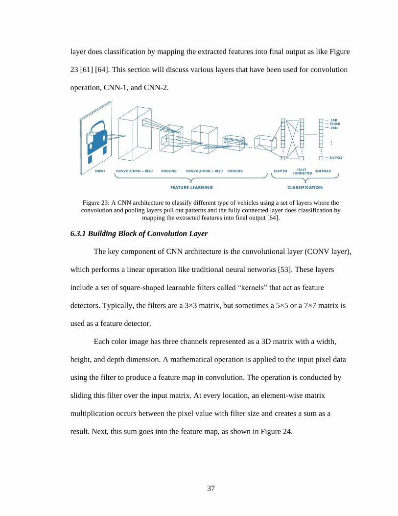
6.3 The Architecture of Deep Convolutional Neural Network
The convolutional neural network (CNN) is a specialized type of neural network
designed to do “convolution” operation of one-dimensional data, two-dimensional data,
and three-dimensional image data [53]. CNN is a mathematical concept composed of
three types of layers convolution, pooling, and fully connected layers. Typically, the
convolution and pooling layers perform feature extraction, whereas the fully connected
37
layer does classification by mapping the extracted features into final output as like Figure
23 [61] [64]. This section will discuss various layers that have been used for convolution
operation, CNN-1, and CNN-2.
Figure 23: A CNN architecture to classify different type of vehicles using a set of layers where the
convolution and pooling layers pull out patterns and the fully connected layer does classification by
mapping the extracted features into final output [64].
6.3.1 Building Block of Convolution Layer
The key component of CNN architecture is the convolutional layer (CONV layer),
which performs a linear operation like traditional neural networks [53]. These layers
include a set of square-shaped learnable filters called “kernels” that act as feature
detectors. Typically, the filters are a 3×3 matrix, but sometimes a 5×5 or a 7×7 matrix is
used as a feature detector.
Each color image has three channels represented as a 3D matrix with a width,
height, and depth dimension. A mathematical operation is applied to the input pixel data
using the filter to produce a feature map in convolution. The operation is conducted by
sliding this filter over the input matrix. At every location, an element-wise matrix
multiplication occurs between the pixel value with filter size and creates a sum as a
result. Next, this sum goes into the feature map, as shown in Figure 24.
38
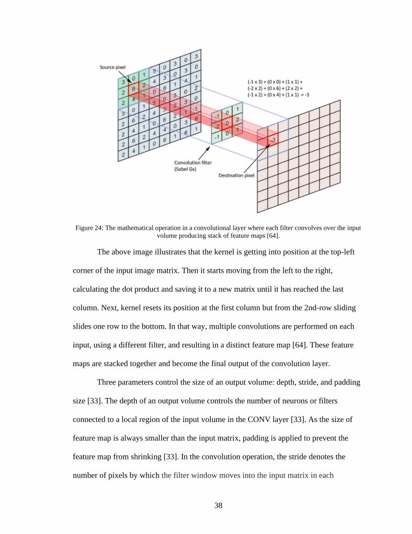
Figure 24: The mathematical operation in a convolutional layer where each filter convolves over the input
volume producing stack of feature maps [64].
The above image illustrates that the kernel is getting into position at the top-left
corner of the input image matrix. Then it starts moving from the left to the right,
calculating the dot product and saving it to a new matrix until it has reached the last
column. Next, kernel resets its position at the first column but from the 2nd-row sliding
slides one row to the bottom. In that way, multiple convolutions are performed on each
input, using a different filter, and resulting in a distinct feature map [64]. These feature
maps are stacked together and become the final output of the convolution layer.
Three parameters control the size of an output volume: depth, stride, and padding
size [33]. The depth of an output volume controls the number of neurons or filters
connected to a local region of the input volume in the CONV layer [33]. As the size of
feature map is always smaller than the input matrix, padding is applied to prevent the
feature map from shrinking [33]. In the convolution operation, the stride denotes the
number of pixels by which the filter window moves into the input matrix in each
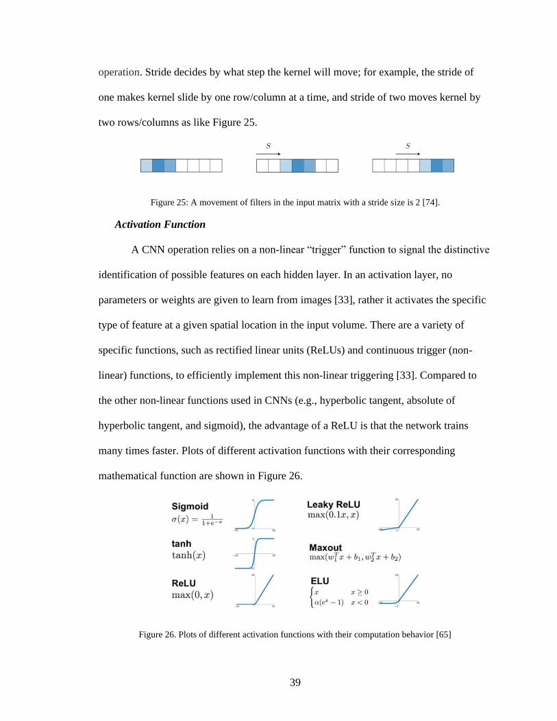
39
operation. Stride decides by what step the kernel will move; for example, the stride of
one makes kernel slide by one row/column at a time, and stride of two moves kernel by
two rows/columns as like Figure 25.
Figure 25: A movement of filters in the input matrix with a stride size is 2 [74].
Activation Function
A CNN operation relies on a non-linear “trigger” function to signal the distinctive
identification of possible features on each hidden layer. In an activation layer, no
parameters or weights are given to learn from images [33], rather it activates the specific
type of feature at a given spatial location in the input volume. There are a variety of
specific functions, such as rectified linear units (ReLUs) and continuous trigger (non-
linear) functions, to efficiently implement this non-linear triggering [33]. Compared to
the other non-linear functions used in CNNs (e.g., hyperbolic tangent, absolute of
hyperbolic tangent, and sigmoid), the advantage of a ReLU is that the network trains
many times faster. Plots of different activation functions with their corresponding
mathematical function are shown in Figure 26.
Figure 26. Plots of different activation functions with their computation behavior [65]
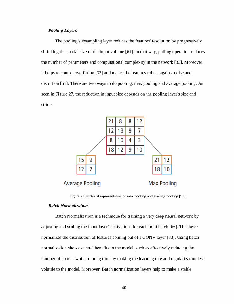
40
Pooling Layers
The pooling/subsampling layer reduces the features' resolution by progressively
shrinking the spatial size of the input volume [61]. In that way, pulling operation reduces
the number of parameters and computational complexity in the network [33]. Moreover,
it helps to control overfitting [33] and makes the features robust against noise and
distortion [51]. There are two ways to do pooling: max pooling and average pooling. As
seen in Figure 27, the reduction in input size depends on the pooling layer's size and
stride.
Figure 27. Pictorial representation of max pooling and average pooling [51]
Batch Normalization
Batch Normalization is a technique for training a very deep neural network by
adjusting and scaling the input layer's activations for each mini batch [66]. This layer
normalizes the distribution of features coming out of a CONV layer [33]. Using batch
normalization shows several benefits to the model, such as effectively reducing the
number of epochs while training time by making the learning rate and regularization less
volatile to the model. Moreover, Batch normalization layers help to make a stable
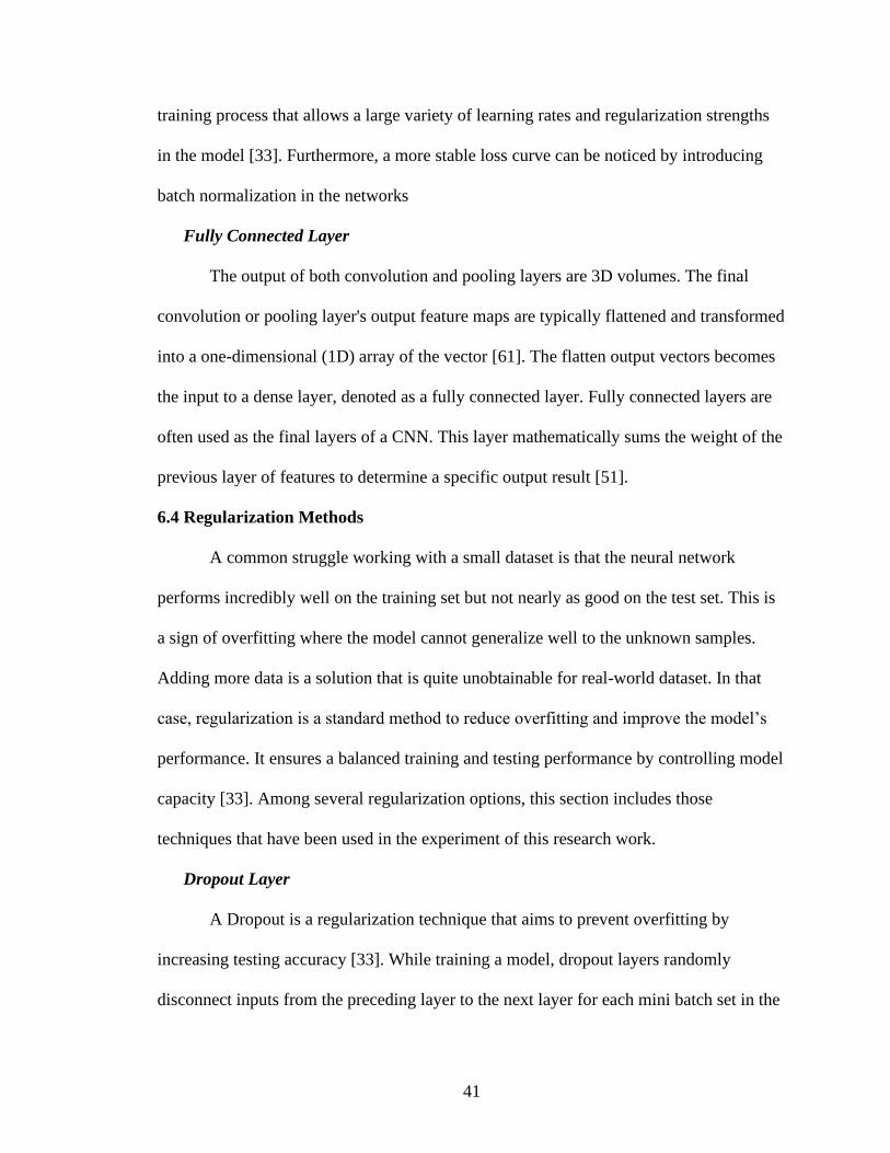
41
training process that allows a large variety of learning rates and regularization strengths
in the model [33]. Furthermore, a more stable loss curve can be noticed by introducing
batch normalization in the networks
Fully Connected Layer
The output of both convolution and pooling layers are 3D volumes. The final
convolution or pooling layer's output feature maps are typically flattened and transformed
into a one-dimensional (1D) array of the vector [61]. The flatten output vectors becomes
the input to a dense layer, denoted as a fully connected layer. Fully connected layers are
often used as the final layers of a CNN. This layer mathematically sums the weight of the
previous layer of features to determine a specific output result [51].
6.4 Regularization Methods
A common struggle working with a small dataset is that the neural network
performs incredibly well on the training set but not nearly as good on the test set. This is
a sign of overfitting where the model cannot generalize well to the unknown samples.
Adding more data is a solution that is quite unobtainable for real-world dataset. In that
case, regularization is a standard method to reduce overfitting and improve the model’s
performance. It ensures a balanced training and testing performance by controlling model
capacity [33]. Among several regularization options, this section includes those
techniques that have been used in the experiment of this research work.
Dropout Layer
A Dropout is a regularization technique that aims to prevent overfitting by
increasing testing accuracy [33]. While training a model, dropout layers randomly
disconnect inputs from the preceding layer to the next layer for each mini batch set in the
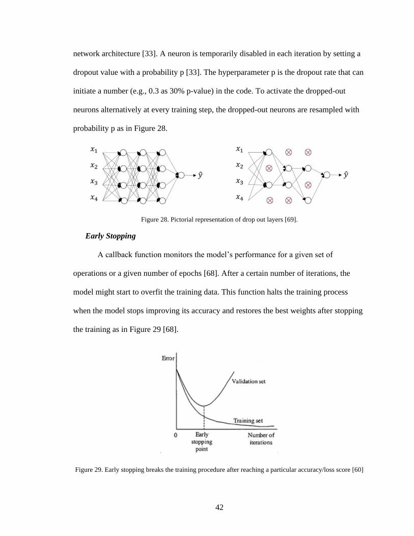
42
network architecture [33]. A neuron is temporarily disabled in each iteration by setting a
dropout value with a probability p [33]. The hyperparameter p is the dropout rate that can
initiate a number (e.g., 0.3 as 30% p-value) in the code. To activate the dropped-out
neurons alternatively at every training step, the dropped-out neurons are resampled with
probability p as in Figure 28.
Figure 28. Pictorial representation of drop out layers [69].
Early Stopping
A callback function monitors the model’s performance for a given set of
operations or a given number of epochs [68]. After a certain number of iterations, the
model might start to overfit the training data. This function halts the training process
when the model stops improving its accuracy and restores the best weights after stopping
the training as in Figure 29 [68].
Figure 29. Early stopping breaks the training procedure after reaching a particular accuracy/loss score [60]
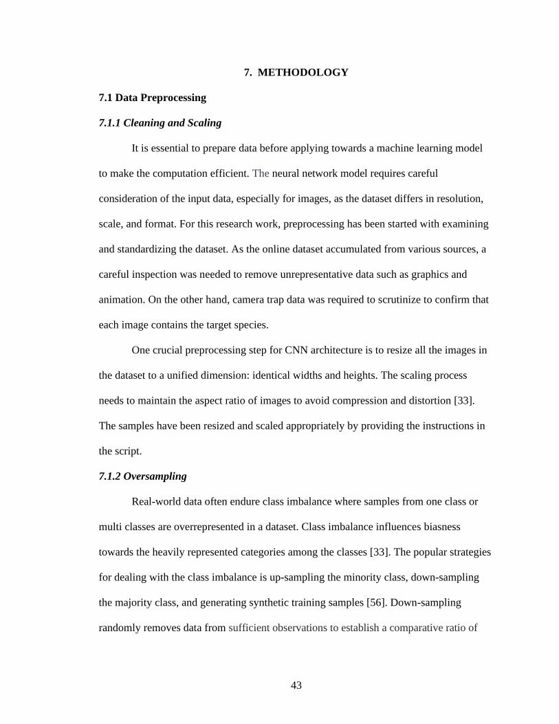
43
7. METHODOLOGY
7.1 Data Preprocessing
7.1.1 Cleaning and Scaling
It is essential to prepare data before applying towards a machine learning model
to make the computation efficient. The neural network model requires careful
consideration of the input data, especially for images, as the dataset differs in resolution,
scale, and format. For this research work, preprocessing has been started with examining
and standardizing the dataset. As the online dataset accumulated from various sources, a
careful inspection was needed to remove unrepresentative data such as graphics and
animation. On the other hand, camera trap data was required to scrutinize to confirm that
each image contains the target species.
One crucial preprocessing step for CNN architecture is to resize all the images in
the dataset to a unified dimension: identical widths and heights. The scaling process
needs to maintain the aspect ratio of images to avoid compression and distortion [33].
The samples have been resized and scaled appropriately by providing the instructions in
the script.
7.1.2 Oversampling
Real-world data often endure class imbalance where samples from one class or
multi classes are overrepresented in a dataset. Class imbalance influences biasness
towards the heavily represented categories among the classes [33]. The popular strategies
for dealing with the class imbalance is up-sampling the minority class, down-sampling
the majority class, and generating synthetic training samples [56]. Down-sampling
randomly removes data from sufficient observations to establish a comparative ratio of
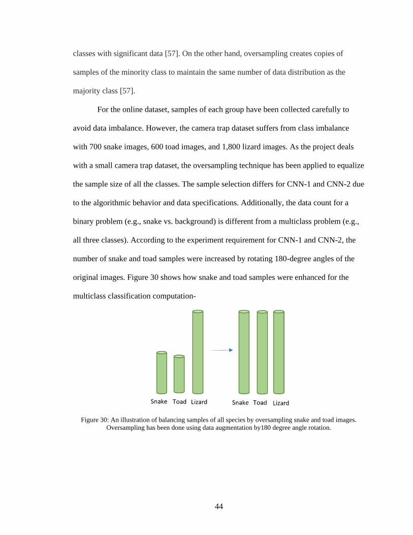
44
classes with significant data [57]. On the other hand, oversampling creates copies of
samples of the minority class to maintain the same number of data distribution as the
majority class [57].
For the online dataset, samples of each group have been collected carefully to
avoid data imbalance. However, the camera trap dataset suffers from class imbalance
with 700 snake images, 600 toad images, and 1,800 lizard images. As the project deals
with a small camera trap dataset, the oversampling technique has been applied to equalize
the sample size of all the classes. The sample selection differs for CNN-1 and CNN-2 due
to the algorithmic behavior and data specifications. Additionally, the data count for a
binary problem (e.g., snake vs. background) is different from a multiclass problem (e.g.,
all three classes). According to the experiment requirement for CNN-1 and CNN-2, the
number of snake and toad samples were increased by rotating 180-degree angles of the
original images. Figure 30 shows how snake and toad samples were enhanced for the
multiclass classification computation-
Figure 30: An illustration of balancing samples of all species by oversampling snake and toad images.
Oversampling has been done using data augmentation by180 degree angle rotation.
45
7.1.3 Augmentation
The image augmentation technique creates data variations synthetically in existing
images to represent a comprehensive set of possible changes [58]. Augmentation will
provide the model a wide range of transformation so that the model learns objects in
various forms and shapes in the training phase [58,59]. This technique also helps to
increase the model’s generalization ability to predict an unseen image of target classes.
Moreover, in some cases, augmentation helps to reduce the overfitting problem [58,59].
Data augmentation can be applied as a pre-processing step in two options: dataset
generation and enlarging an existing dataset, and on-the-fly data augmentation [59]. The
difference between the two methods relies on the data enlargement procedure and the
implementation time. The dataset generation is an additive process to expand the existing
dataset whereas, on-the-fly data augmentation using Keras ImageDataGenerator does not
combine the transformed data into the original dataset. It just performed with the
modified data while training time.
To achieve a relative class balance and to improve the generalization ability of a
model, both the augmentation actions have been applied in the thesis work. Although, on-
the-fly data augmentation has been introduced only in CNN-2, which distinguish the
computation behavior between two models. Below subsections describe two
augmentation process elaborately.
Data generation: In this method, the dataset is expanded by adding slightly transformed
samples to the existing directory. This is an offline process that is usually applied for a small
dataset. The steps are –
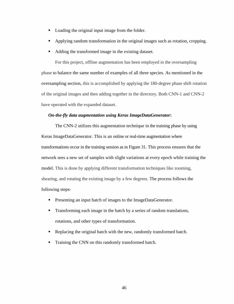
46
▪ Loading the original input image from the folder.
▪ Applying random transformation in the original images such as rotation, cropping.
▪ Adding the transformed image in the existing dataset.
For this project, offline augmentation has been employed in the oversampling
phase to balance the same number of examples of all three species. As mentioned in the
oversampling section, this is accomplished by applying the 180-degree phase shift rotation
of the original images and then adding together in the directory. Both CNN-1 and CNN-2
have operated with the expanded dataset.
On-the-fly data augmentation using Keras ImageDataGenerator:
The CNN-2 utilizes this augmentation technique in the training phase by using
Keras ImageDataGenerator. This is an online or real-time augmentation where
transformations occur in the training session as in Figure 31. This process ensures that the
network sees a new set of samples with slight variations at every epoch while training the
model. This is done by applying different transformation techniques like zooming,
shearing, and rotating the existing image by a few degrees. The process follows the
following steps-
▪ Presenting an input batch of images to the ImageDataGenerator.
▪ Transforming each image in the batch by a series of random translations,
rotations, and other types of transformation.
▪ Replacing the original batch with the new, randomly transformed batch.
▪ Training the CNN on this randomly transformed batch.
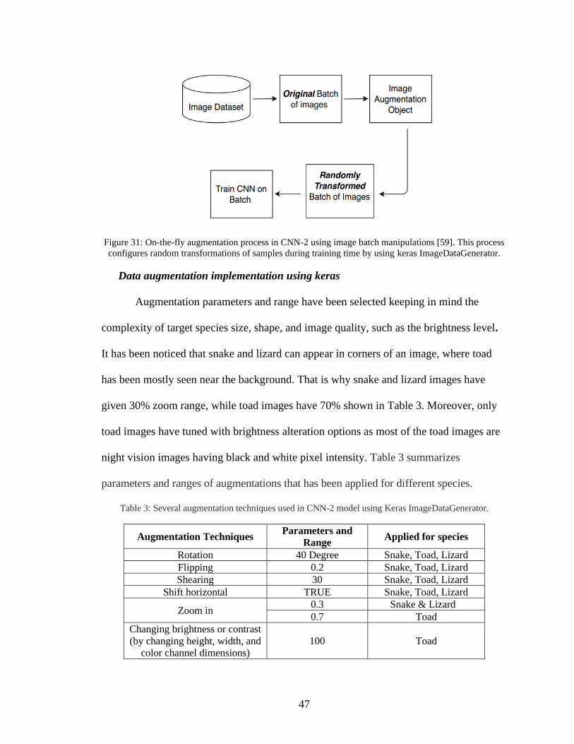
47
Figure 31: On-the-fly augmentation process in CNN-2 using image batch manipulations [59]. This process
configures random transformations of samples during training time by using keras ImageDataGenerator.
Data augmentation implementation using keras
Augmentation parameters and range have been selected keeping in mind the
complexity of target species size, shape, and image quality, such as the brightness level.
It has been noticed that snake and lizard can appear in corners of an image, where toad
has been mostly seen near the background. That is why snake and lizard images have
given 30% zoom range, while toad images have 70% shown in Table 3. Moreover, only
toad images have tuned with brightness alteration options as most of the toad images are
night vision images having black and white pixel intensity. Table 3 summarizes
parameters and ranges of augmentations that has been applied for different species.
Table 3: Several augmentation techniques used in CNN-2 model using Keras ImageDataGenerator.
Augmentation Techniques Parameters and
Range Applied for species
Rotation 40 Degree Snake, Toad, Lizard
Flipping 0.2 Snake, Toad, Lizard
Shearing 30 Snake, Toad, Lizard
Shift horizontal TRUE Snake, Toad, Lizard
Zoom in 0.3 Snake & Lizard
0.7 Toad
Changing brightness or contrast
(by changing height, width, and
color channel dimensions)
100 Toad
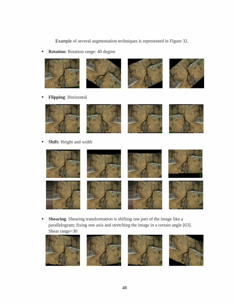
48
Example of several augmentation techniques is represented in Figure 32.
▪ Rotation: Rotation range: 40 degree
▪ Flipping: Horizontal
▪ Shift: Height and width
▪ Shearing: Shearing transformation is shifting one part of the image like a
parallelogram; fixing one axis and stretching the image in a certain angle [63].
Shear range=30
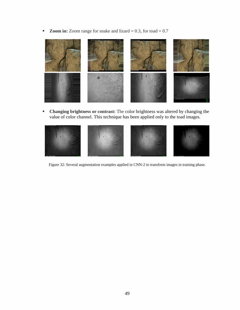
49
▪ Zoom in: Zoom range for snake and lizard = 0.3, for toad = 0.7
▪ Changing brightness or contrast: The color brightness was altered by changing the
value of color channel. This technique has been applied only to the toad images.
Figure 32: Several augmentation examples applied in CNN-2 to transform images in training phase.
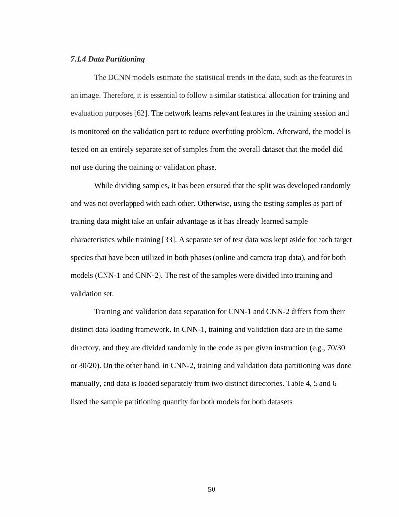
50
7.1.4 Data Partitioning
The DCNN models estimate the statistical trends in the data, such as the features in
an image. Therefore, it is essential to follow a similar statistical allocation for training and
evaluation purposes [62]. The network learns relevant features in the training session and
is monitored on the validation part to reduce overfitting problem. Afterward, the model is
tested on an entirely separate set of samples from the overall dataset that the model did
not use during the training or validation phase.
While dividing samples, it has been ensured that the split was developed randomly
and was not overlapped with each other. Otherwise, using the testing samples as part of
training data might take an unfair advantage as it has already learned sample
characteristics while training [33]. A separate set of test data was kept aside for each target
species that have been utilized in both phases (online and camera trap data), and for both
models (CNN-1 and CNN-2). The rest of the samples were divided into training and
validation set.
Training and validation data separation for CNN-1 and CNN-2 differs from their
distinct data loading framework. In CNN-1, training and validation data are in the same
directory, and they are divided randomly in the code as per given instruction (e.g., 70/30
or 80/20). On the other hand, in CNN-2, training and validation data partitioning was done
manually, and data is loaded separately from two distinct directories. Table 4, 5 and 6
listed the sample partitioning quantity for both models for both datasets.
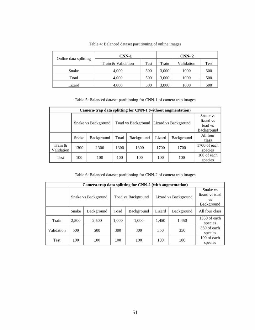
51
Table 4: Balanced dataset partitioning of online images
Online data splitting CNN-1 CNN- 2
Train & Validation Test Train Validation Test
Snake 4,000 500 3,000 1000 500
Toad 4,000 500 3,000 1000 500
Lizard 4,000 500 3,000 1000 500
Table 5: Balanced dataset partitioning for CNN-1 of camera trap images
Camera-trap data splitting for CNN-1 (without augmentation)
Snake vs Background Toad vs Background Lizard vs Background
Snake vs
lizard vs
toad vs
Background
Snake Background Toad Background Lizard Background All four
class
Train &
Validation 1300 1300 1300 1300 1700 1700
1700 of each
species
Test 100 100 100 100 100 100 100 of each
species
Table 6: Balanced dataset partitioning for CNN-2 of camera trap images
Camera-trap data splitting for CNN-2 (with augmentation)
Snake vs Background Toad vs Background Lizard vs Background
Snake vs
lizard vs toad
vs
Background
Snake Background Toad Background Lizard Background All four class
Train 2,500 2,500 1,000 1,000 1,450 1,450 1350 of each
species
Validation 500 500 300 300 350 350 350 of each
species
Test 100 100 100 100 100 100 100 of each
species
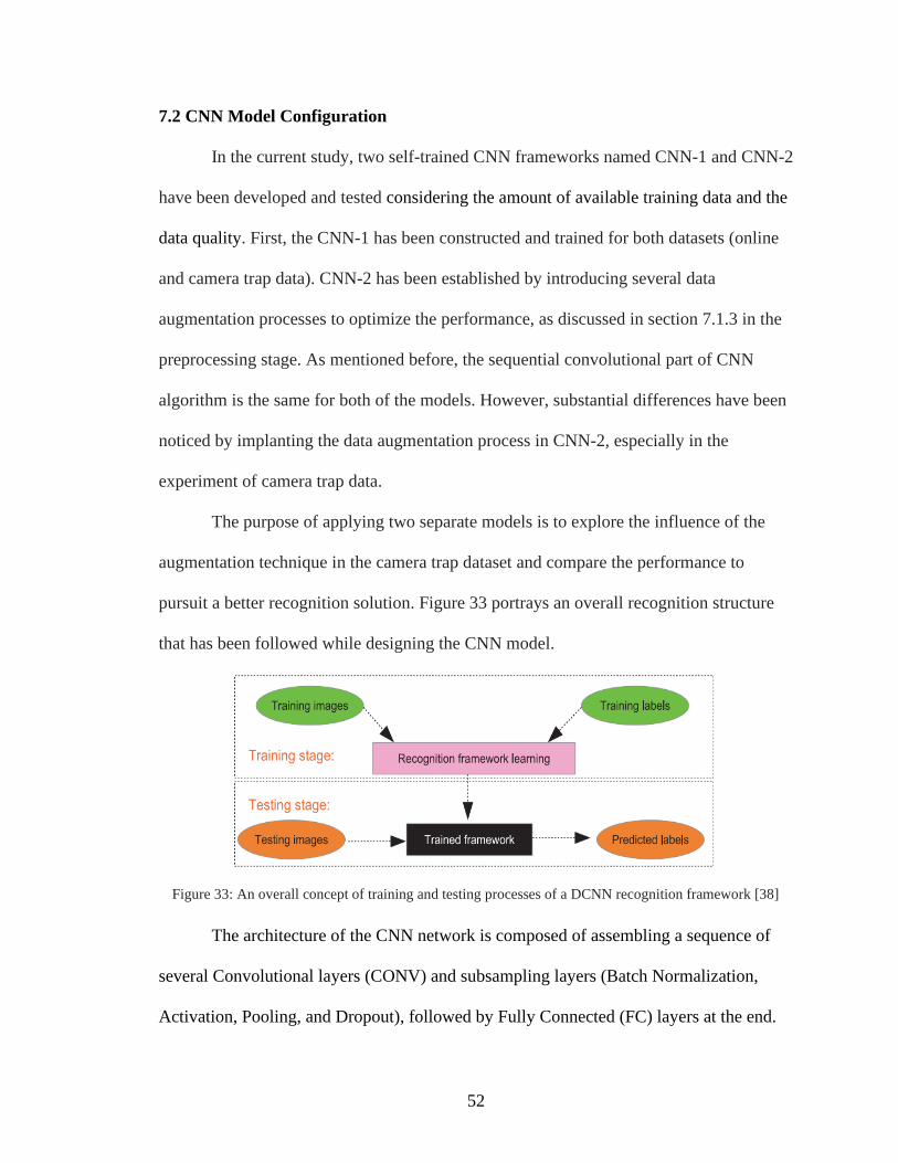
52
7.2 CNN Model Configuration
In the current study, two self-trained CNN frameworks named CNN-1 and CNN-2
have been developed and tested considering the amount of available training data and the
data quality. First, the CNN-1 has been constructed and trained for both datasets (online
and camera trap data). CNN-2 has been established by introducing several data
augmentation processes to optimize the performance, as discussed in section 7.1.3 in the
preprocessing stage. As mentioned before, the sequential convolutional part of CNN
algorithm is the same for both of the models. However, substantial differences have been
noticed by implanting the data augmentation process in CNN-2, especially in the
experiment of camera trap data.
The purpose of applying two separate models is to explore the influence of the
augmentation technique in the camera trap dataset and compare the performance to
pursuit a better recognition solution. Figure 33 portrays an overall recognition structure
that has been followed while designing the CNN model.
Figure 33: An overall concept of training and testing processes of a DCNN recognition framework [38]
The architecture of the CNN network is composed of assembling a sequence of
several Convolutional layers (CONV) and subsampling layers (Batch Normalization,
Activation, Pooling, and Dropout), followed by Fully Connected (FC) layers at the end.
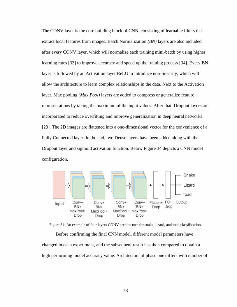
53
The CONV layer is the core building block of CNN, consisting of learnable filters that
extract local features from images. Batch Normalization (BN) layers are also included
after every CONV layer, which will normalize each training mini-batch by using higher
learning rates [33] to improve accuracy and speed up the training process [34]. Every BN
layer is followed by an Activation layer ReLU to introduce non-linearity, which will
allow the architecture to learn complex relationships in the data. Next to the Activation
layer, Max pooling (Max Pool) layers are added to compress or generalize feature
representations by taking the maximum of the input values. After that, Dropout layers are
incorporated to reduce overfitting and improve generalization in deep neural networks
[23]. The 2D images are flattened into a one-dimensional vector for the convenience of a
Fully Connected layer. In the end, two Dense layers have been added along with the
Dropout layer and sigmoid activation function. Below Figure 34 depicts a CNN model
configuration.
Figure 34: An example of four layers CONV architecture for snake, lizard, and toad classification.
Before confirming the final CNN model, different model parameters have
changed in each experiment, and the subsequent result has then compared to obtain a
high performing model accuracy value. Architecture of phase one differs with number of
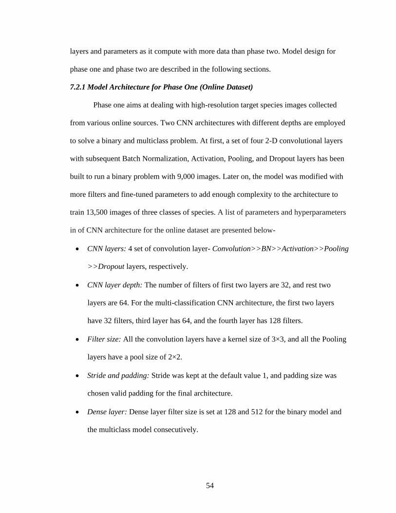
54
layers and parameters as it compute with more data than phase two. Model design for
phase one and phase two are described in the following sections.
7.2.1 Model Architecture for Phase One (Online Dataset)
Phase one aims at dealing with high-resolution target species images collected
from various online sources. Two CNN architectures with different depths are employed
to solve a binary and multiclass problem. At first, a set of four 2-D convolutional layers
with subsequent Batch Normalization, Activation, Pooling, and Dropout layers has been
built to run a binary problem with 9,000 images. Later on, the model was modified with
more filters and fine-tuned parameters to add enough complexity to the architecture to
train 13,500 images of three classes of species. A list of parameters and hyperparameters
in of CNN architecture for the online dataset are presented below-
• CNN layers: 4 set of convolution layer- Convolution>>BN>>Activation>>Pooling
>>Dropout layers, respectively.
• CNN layer depth: The number of filters of first two layers are 32, and rest two
layers are 64. For the multi-classification CNN architecture, the first two layers
have 32 filters, third layer has 64, and the fourth layer has 128 filters.
• Filter size: All the convolution layers have a kernel size of 3×3, and all the Pooling
layers have a pool size of 2×2.
• Stride and padding: Stride was kept at the default value 1, and padding size was
chosen valid padding for the final architecture.
• Dense layer: Dense layer filter size is set at 128 and 512 for the binary model and
the multiclass model consecutively.
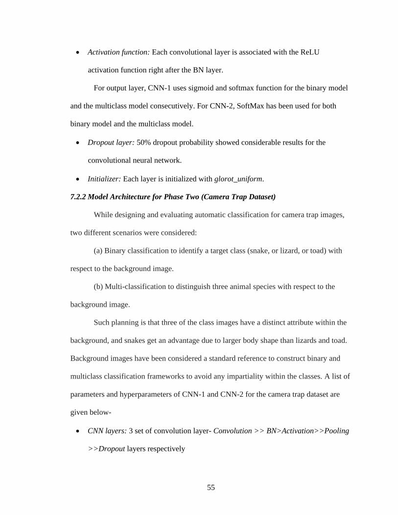
55
• Activation function: Each convolutional layer is associated with the ReLU
activation function right after the BN layer.
For output layer, CNN-1 uses sigmoid and softmax function for the binary model
and the multiclass model consecutively. For CNN-2, SoftMax has been used for both
binary model and the multiclass model.
• Dropout layer: 50% dropout probability showed considerable results for the
convolutional neural network.
• Initializer: Each layer is initialized with glorot_uniform.
7.2.2 Model Architecture for Phase Two (Camera Trap Dataset)
While designing and evaluating automatic classification for camera trap images,
two different scenarios were considered:
(a) Binary classification to identify a target class (snake, or lizard, or toad) with
respect to the background image.
(b) Multi-classification to distinguish three animal species with respect to the
background image.
Such planning is that three of the class images have a distinct attribute within the
background, and snakes get an advantage due to larger body shape than lizards and toad.
Background images have been considered a standard reference to construct binary and
multiclass classification frameworks to avoid any impartiality within the classes. A list of
parameters and hyperparameters of CNN-1 and CNN-2 for the camera trap dataset are
given below-
• CNN layers: 3 set of convolution layer- Convolution >> BN>Activation>>Pooling
>>Dropout layers respectively
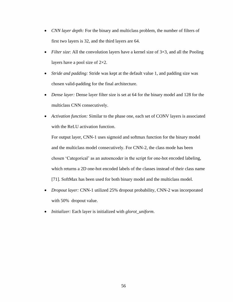
56
• CNN layer depth: For the binary and multiclass problem, the number of filters of
first two layers is 32, and the third layers are 64.
• Filter size: All the convolution layers have a kernel size of 3×3, and all the Pooling
layers have a pool size of 2×2.
• Stride and padding: Stride was kept at the default value 1, and padding size was
chosen valid-padding for the final architecture.
• Dense layer: Dense layer filter size is set at 64 for the binary model and 128 for the
multiclass CNN consecutively.
• Activation function: Similar to the phase one, each set of CONV layers is associated
with the ReLU activation function.
For output layer, CNN-1 uses sigmoid and softmax function for the binary model
and the multiclass model consecutively. For CNN-2, the class mode has been
chosen ‘Categorical’ as an autoencoder in the script for one-hot encoded labeling,
which returns a 2D one-hot encoded labels of the classes instead of their class name
[71]. SoftMax has been used for both binary model and the multiclass model.
• Dropout layer: CNN-1 utilized 25% dropout probability, CNN-2 was incorporated
with 50% dropout value.
• Initializer: Each layer is initialized with glorot_uniform.
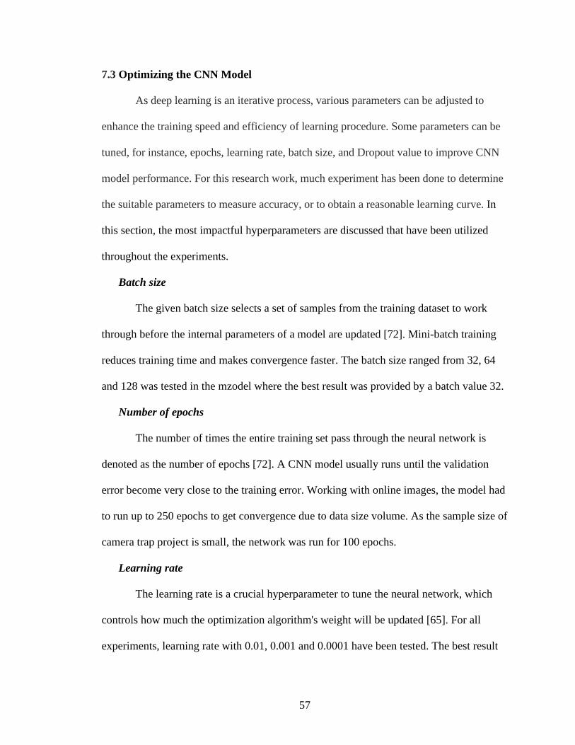
57
7.3 Optimizing the CNN Model
As deep learning is an iterative process, various parameters can be adjusted to
enhance the training speed and efficiency of learning procedure. Some parameters can be
tuned, for instance, epochs, learning rate, batch size, and Dropout value to improve CNN
model performance. For this research work, much experiment has been done to determine
the suitable parameters to measure accuracy, or to obtain a reasonable learning curve. In
this section, the most impactful hyperparameters are discussed that have been utilized
throughout the experiments.
Batch size
The given batch size selects a set of samples from the training dataset to work
through before the internal parameters of a model are updated [72]. Mini-batch training
reduces training time and makes convergence faster. The batch size ranged from 32, 64
and 128 was tested in the mzodel where the best result was provided by a batch value 32.
Number of epochs
The number of times the entire training set pass through the neural network is
denoted as the number of epochs [72]. A CNN model usually runs until the validation
error become very close to the training error. Working with online images, the model had
to run up to 250 epochs to get convergence due to data size volume. As the sample size of
camera trap project is small, the network was run for 100 epochs.
Learning rate
The learning rate is a crucial hyperparameter to tune the neural network, which
controls how much the optimization algorithm's weight will be updated [65]. For all
experiments, learning rate with 0.01, 0.001 and 0.0001 have been tested. The best result
58
for online and CNN-2 was achieved with a keras default learning rate of 0.01 and for
CNN-1 experiment, the learning rate was 0.0001.
Dropout for regularization
In order to battle with overfitting, Dropout values were also tuned after each
Convolution and Fully Connected layer. For online images, the dropout value was kept
0.5 for all the layers. For the experiment of camera trap images with CNN-1 model, the
best accuracy was achieved with a dropout value of 0.25 after the Convolutional layers
and a 0.5 dropout value after the Fully Connected layer. The learning curve of CNN-2
experiments were suffering from overfitting problem, the dropout value was kept at 0.5
for all the layers.
7.4 Computational Tools and Environment
For this project's writing script, the Python programming language was utilized
using deep learning libraries such as Keras, Numpy, Scikit-learn, and Matplotlib. Python
is a flexible, intuitive syntax [33] that allows developers to build, test, and tweak a model
efficiently. Essential image processing operations such as loading images from disk and
displaying them to our screen were performed with OpenCV standard library.
After building the initial architecture, the model was run multiple times in the
LEAP cluster, a high-performance computing cluster facilitated by Texas State
University. LEAP stands for “Learning, Exploration, Analysis, and Processing,” which is
configured with 28 CPU cores, Dual 2.4 GHz E5- 2680v4 Intel Xeon (Broadwell)
processors, 15 TBs of memory, and 48 TBs of local storage in total [73]. High throughput
analysis was achieved using the cluster by submitting parallel jobs to evaluate the
optimized hyperparameters.
59
8. EXPERIMENT AND RESULT ANALYSIS
8.1. Experiment and Result Analysis for Phase One (Online Dataset)
Though the goal of the research work is to recognize wild animal species from a
large camera trap dataset, the initial work started with building and training a CNN
classifier with online images. The aim was to create a binary and multiclass recognition
system prototype for future implementation using real-world datasets. The initial work
helped to get familiarized with the concept of classification using DCNN and understand
computer vision analysis with image data. Once the model was constructed, it has been
utilized for the camera trap data, where the previous models were fine-tuned according to
the desired output.
A binary and a multiclass structure were experimented with two CNN models
with 4,500 online images of each group (snake, lizard, and toad). As an example of a
binary recognition problem, a model has been developed with toad and snake species.
Later, the work was extended by adding lizard as a class. The experiment results were
compared within the group of species and also between the models (CNN-1 and CNN-2
architectures) as described in below subsections.
60
A) Binary Classification Result (Toad And Snake)
In the initial stage, the research work started with building a binary classification
model (CNN-1) of snake and toad with 414 images of each species from the Caltech
dataset. The model was composed of CONV layers with activation ReLU function, 2x2
MAX Pooling layers, added with Dropout layers. The model got overfitted after 30
epochs due to the limited imagery samples (828 total images). The best training and
validation accuracy of that CNN-1 model was 67% and 60%, respectively [70].
A reasonable extension of that binary experiment has been conducted to improve
the performance by adding more images into the dataset. The model is trained and
validated with a balanced two-class image dataset consisting of 8,000 images where 70%
of data has been utilized for training, 30% is for validation. A separate sample set of
1,000 images has been utilized for testing purpose. The input data sizes varied in different
resolutions in the RGB channel, but images were scaled down to 100 pixels in greyscale
to reduce computational time and complicacy.
Many changes have made in the architecture, such as changing layers, filter count,
drop out value, and other parameters to the previous model considering the data size.
Also, a Batch normalization layer and initializer were introduced to the model.
The below training and validation loss and accuracy curves in Figure 1 illustrate
the learning performance changes over time. As expected, the validation curve decreases,
followed by the training curve for 200 iterations. Both the training and validation loss
decreases with a minimal gap between the two final loss values indicating a fitted model.
Both curves have fluctuation because the model is changing its prediction as plotted in
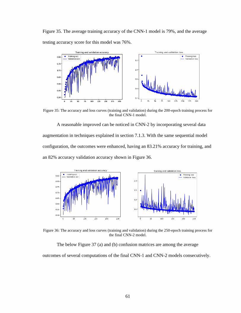
61
Figure 35. The average training accuracy of the CNN-1 model is 79%, and the average
testing accuracy score for this model was 76%.
Figure 35: The accuracy and loss curves (training and validation) during the 200-epoch training process for
the final CNN-1 model.
A reasonable improved can be noticed in CNN-2 by incorporating several data
augmentation in techniques explained in section 7.1.3. With the same sequential model
configuration, the outcomes were enhanced, having an 83.21% accuracy for training, and
an 82% accuracy validation accuracy shown in Figure 36.
Figure 36: The accuracy and loss curves (training and validation) during the 250-epoch training process for
the final CNN-2 model.
The below Figure 37 (a) and (b) confusion matrices are among the average
outcomes of several computations of the final CNN-1 and CNN-2 models consecutively.
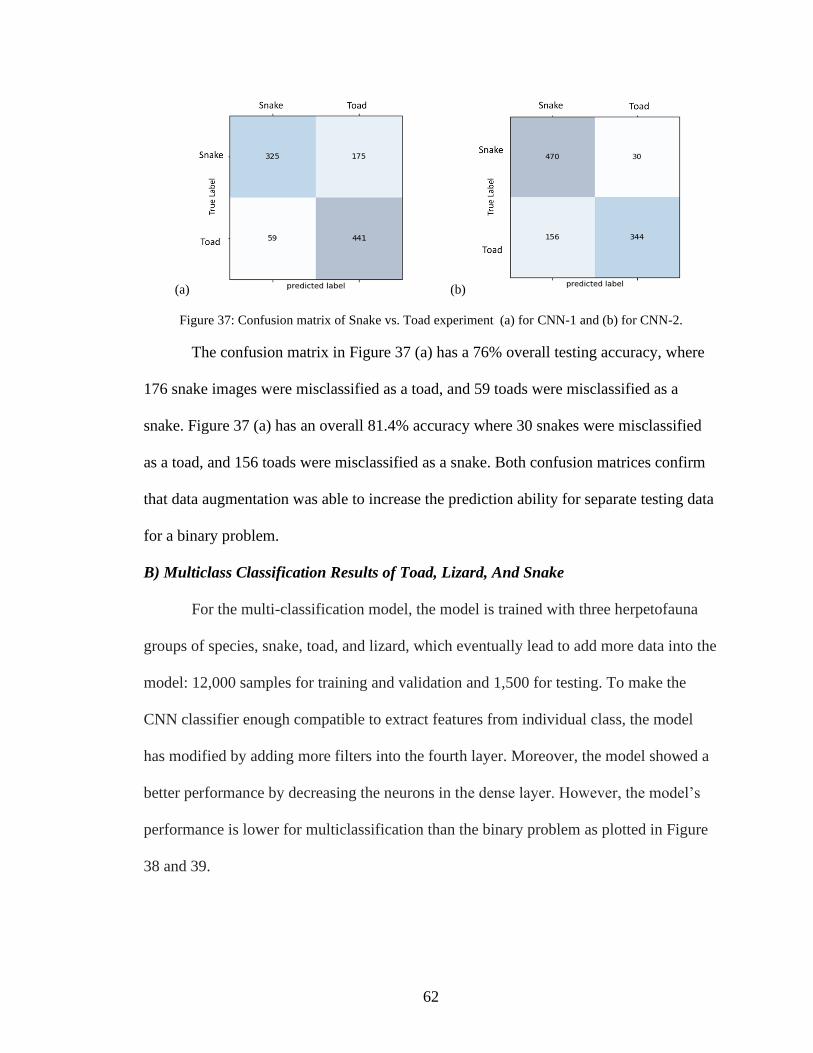
62
(a) (b)
Figure 37: Confusion matrix of Snake vs. Toad experiment (a) for CNN-1 and (b) for CNN-2.
The confusion matrix in Figure 37 (a) has a 76% overall testing accuracy, where
176 snake images were misclassified as a toad, and 59 toads were misclassified as a
snake. Figure 37 (a) has an overall 81.4% accuracy where 30 snakes were misclassified
as a toad, and 156 toads were misclassified as a snake. Both confusion matrices confirm
that data augmentation was able to increase the prediction ability for separate testing data
for a binary problem.
B) Multiclass Classification Results of Toad, Lizard, And Snake
For the multi-classification model, the model is trained with three herpetofauna
groups of species, snake, toad, and lizard, which eventually lead to add more data into the
model: 12,000 samples for training and validation and 1,500 for testing. To make the
CNN classifier enough compatible to extract features from individual class, the model
has modified by adding more filters into the fourth layer. Moreover, the model showed a
better performance by decreasing the neurons in the dense layer. However, the model’s
performance is lower for multiclassification than the binary problem as plotted in Figure
38 and 39.
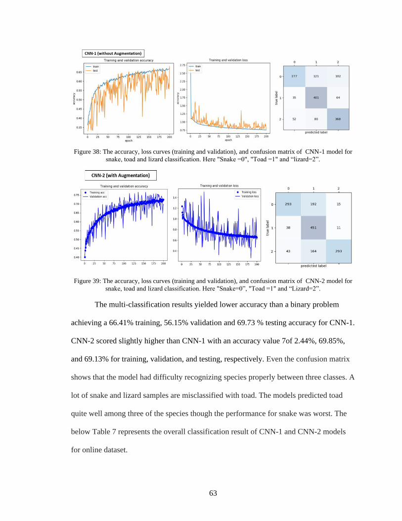
63
Figure 38: The accuracy, loss curves (training and validation), and confusion matrix of CNN-1 model for
snake, toad and lizard classification. Here "Snake =0", "Toad =1" and “lizard=2”.
Figure 39: The accuracy, loss curves (training and validation), and confusion matrix of CNN-2 model for
snake, toad and lizard classification. Here "Snake=0”, "Toad =1" and “Lizard=2”.
The multi-classification results yielded lower accuracy than a binary problem
achieving a 66.41% training, 56.15% validation and 69.73 % testing accuracy for CNN-1.
CNN-2 scored slightly higher than CNN-1 with an accuracy value 7of 2.44%, 69.85%,
and 69.13% for training, validation, and testing, respectively. Even the confusion matrix
shows that the model had difficulty recognizing species properly between three classes. A
lot of snake and lizard samples are misclassified with toad. The models predicted toad
quite well among three of the species though the performance for snake was worst. The
below Table 7 represents the overall classification result of CNN-1 and CNN-2 models
for online dataset.
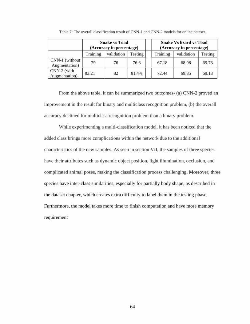
64
Table 7: The overall classification result of CNN-1 and CNN-2 models for online dataset.
Snake vs Toad
(Accuracy in percentage)
Snake Vs lizard vs Toad
(Accuracy in percentage)
Training validation Testing Training validation Testing
CNN-1 (without
Augmentation) 79 76 76.6 67.18 68.08 69.73
CNN-2 (with
Augmentation) 83.21 82 81.4% 72.44 69.85 69.13
From the above table, it can be summarized two outcomes- (a) CNN-2 proved an
improvement in the result for binary and multiclass recognition problem, (b) the overall
accuracy declined for multiclass recognition problem than a binary problem.
While experimenting a multi-classification model, it has been noticed that the
added class brings more complications within the network due to the additional
characteristics of the new samples. As seen in section VII, the samples of three species
have their attributes such as dynamic object position, light illumination, occlusion, and
complicated animal poses, making the classification process challenging. Moreover, three
species have inter-class similarities, especially for partially body shape, as described in
the dataset chapter, which creates extra difficulty to label them in the testing phase.
Furthermore, the model takes more time to finish computation and have more memory
requirement
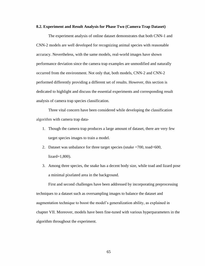
65
8.2. Experiment and Result Analysis for Phase Two (Camera Trap Dataset)
The experiment analysis of online dataset demonstrates that both CNN-1 and
CNN-2 models are well developed for recognizing animal species with reasonable
accuracy. Nevertheless, with the same models, real-world images have shown
performance deviation since the camera trap examples are unmodified and naturally
occurred from the environment. Not only that, both models, CNN-2 and CNN-2
performed differently providing a different set of results. However, this section is
dedicated to highlight and discuss the essential experiments and corresponding result
analysis of camera trap species classification.
Three vital concern have been considered while developing the classification
algorithm with camera trap data-
1. Though the camera trap produces a large amount of dataset, there are very few
target species images to train a model.
2. Dataset was unbalance for three target species (snake =700, toad=600,
lizard=1,800).
3. Among three species, the snake has a decent body size, while toad and lizard pose
a minimal pixelated area in the background.
First and second challenges have been addressed by incorporating preprocessing
techniques to a dataset such as oversampling images to balance the dataset and
augmentation technique to boost the model’s generalization ability, as explained in
chapter VII. Moreover, models have been fine-tuned with various hyperparameters in the
algorithm throughout the experiment.
66
All three species have been classified individually regarding background images
producing three separate binary problems; ‘lizard vs. background,’ ‘toad vs. background,’
and ‘snake vs. background’ to find a logical solution of third concern. Background
samples can be referred to as images that do not contain any of the three target species in
that data point. A new label of dataset named ‘background’ has been formed from camera
trap images with the same resolution and environment condition as the other data
examples. In the end, all four sets of labeled data have experimented together CNN-1 and
CNN-2, and results were compared for a better understanding of recognition
performance.
A model’s performance can be evaluated on how the classifier will recognize new
or unseen data from the same distribution of samples used to train the model. This can
also be defined as the generalization ability of a CNN classifier. For camera trap images,
after training the model, the performance has been validated with a given set of samples
that measure how well the model is generalizing the trained class. The classification
evaluation was done with a separate set of the testing dataset. The test result has been
used to plot a confusion matrix that summarizes the prediction of classification results,
including correct and incorrect label estimation.
Along with the learning curve and confusion matrix, the model will predict an
unseen image from the saved model. After training, the model was saved using Keras
function model.Save, where the saved model will store the weights and architecture in
separate files. Utilizing the load_model function, the model is directly used to predict a
new image that the model has never faced in training and testing. For that testing
purpose, a completely isolated set of samples of 10 images of each species has been
67
separated and later applied to test the model’s generalization ability. The subsequent
sections will describe the result analysis of CNN-1 and CNN-2 separately.
8.2.1 Performance Evaluation of CNN-1 (Without Augmentation)
In CNN-1, training and validation samples were loaded together from the same
directory and split randomly by instruction in the algorithm. Due to the small sample size
of 1,300 for training and validation of each species, 80% was used to train the model, and
20% for validation of the training. The input size of images is 150 pixels that were
converted into greyscale before feeding into the model. A separate set of 100 images was
used to predict species' label as a form of the classification performance.
The model was optimized by adjusting several hyperparameters such as batch
size, number of epochs, kernel size, the filter number, learning rate, and Dropout
percentage. For tuning, the Dropout layer with a value range of 0.25 to 0.75 was varied,
where 0.25 showed a favorable outcome after the CONV layer and 0.5 after the Dense
layer. The architecture was compiled with the categorical cross-entropy loss function.
After trying out several learning rates such as 0.01, 0.001, and 0.0001 of Adam optimizer,
the final rate was selected as 0.0001. With the combination of 32 batch size, the
computation was executed for 100 epochs. Each of the results is represented in below
plot 40, 41, and 42 with the learning curve and confusion matrix.

68
Toad Vs Background
(a) (b)
Figure 40: (a) The accuracy, loss curves (training and validation) with respect to the number of epochs, and
(b) confusion matrix of the final CNN-1 model for toad vs background of camera trap images.
Lizard Vs Background
(a) (b)
Figure 41: (a) The accuracy, loss curves (training and validation) with respect to the number of epochs, and
(b) confusion matrix of the final CNN-1 model for lizard vs background of camera trap images.
Snake vs Background
(a) (b)
Figure 42: (a) The accuracy, loss curves (training and validation) with respect to the number of epochs, and
(b) confusion matrix of the final CNN-1 model for snake vs background of camera trap images.
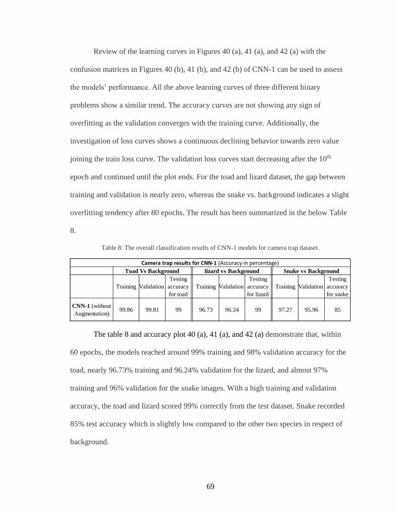
69
Review of the learning curves in Figures 40 (a), 41 (a), and 42 (a) with the
confusion matrices in Figures 40 (b), 41 (b), and 42 (b) of CNN-1 can be used to assess
the models’ performance. All the above learning curves of three different binary
problems show a similar trend. The accuracy curves are not showing any sign of
overfitting as the validation converges with the training curve. Additionally, the
investigation of loss curves shows a continuous declining behavior towards zero value
joining the train loss curve. The validation loss curves start decreasing after the 10th
epoch and continued until the plot ends. For the toad and lizard dataset, the gap between
training and validation is nearly zero, whereas the snake vs. background indicates a slight
overfitting tendency after 80 epochs. The result has been summarized in the below Table
8.
Table 8: The overall classification results of CNN-1 models for camera trap dataset.
The table 8 and accuracy plot 40 (a), 41 (a), and 42 (a) demonstrate that, within
60 epochs, the models reached around 99% training and 98% validation accuracy for the
toad, nearly 96.73% training and 96.24% validation for the lizard, and almost 97%
training and 96% validation for the snake images. With a high training and validation
accuracy, the toad and lizard scored 99% correctly from the test dataset. Snake recorded
85% test accuracy which is slightly low compared to the other two species in respect of
background.
Training Validation
Testing
accuracy
for toad
Training Validation
Testing
accuracy
for lizard
Training Validation
Testing
accuracy
for snake
CNN-1 (without
Augmentation)99.86 99.81 99 96.73 96.24 99 97.27 95.96 85
lizard vs Background Snake vs Background
Camera trap results for CNN-1 (Accuracy in percentage)
Toad Vs Background
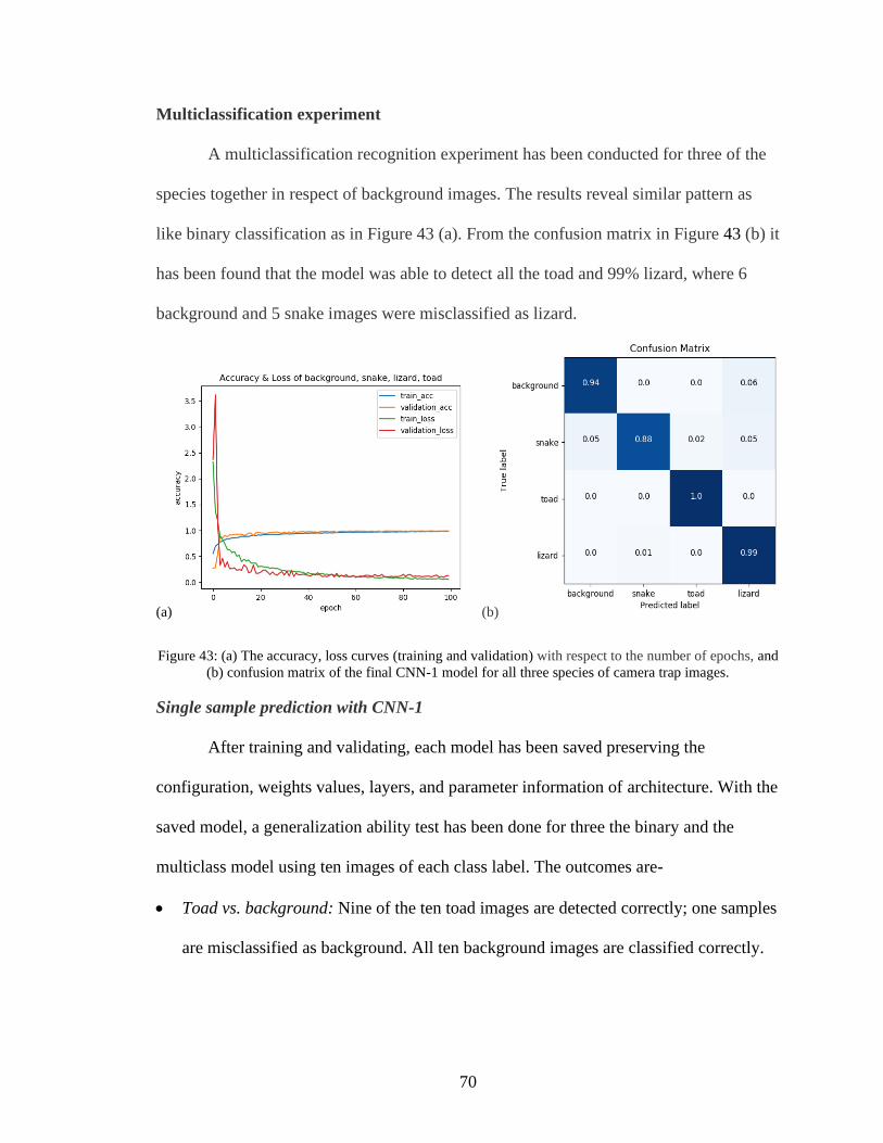
70
Multiclassification experiment
A multiclassification recognition experiment has been conducted for three of the
species together in respect of background images. The results reveal similar pattern as
like binary classification as in Figure 43 (a). From the confusion matrix in Figure 43 (b) it
has been found that the model was able to detect all the toad and 99% lizard, where 6
background and 5 snake images were misclassified as lizard.
(a) (b)
Figure 43: (a) The accuracy, loss curves (training and validation) with respect to the number of epochs, and
(b) confusion matrix of the final CNN-1 model for all three species of camera trap images.
Single sample prediction with CNN-1
After training and validating, each model has been saved preserving the
configuration, weights values, layers, and parameter information of architecture. With the
saved model, a generalization ability test has been done for three the binary and the
multiclass model using ten images of each class label. The outcomes are-
• Toad vs. background: Nine of the ten toad images are detected correctly; one samples
are misclassified as background. All ten background images are classified correctly.
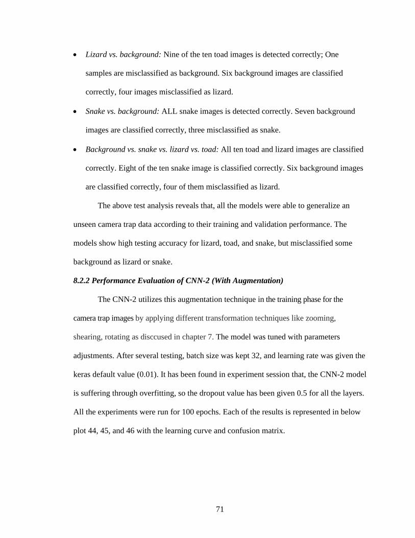
71
• Lizard vs. background: Nine of the ten toad images is detected correctly; One
samples are misclassified as background. Six background images are classified
correctly, four images misclassified as lizard.
• Snake vs. background: ALL snake images is detected correctly. Seven background
images are classified correctly, three misclassified as snake.
• Background vs. snake vs. lizard vs. toad: All ten toad and lizard images are classified
correctly. Eight of the ten snake image is classified correctly. Six background images
are classified correctly, four of them misclassified as lizard.
The above test analysis reveals that, all the models were able to generalize an
unseen camera trap data according to their training and validation performance. The
models show high testing accuracy for lizard, toad, and snake, but misclassified some
background as lizard or snake.
8.2.2 Performance Evaluation of CNN-2 (With Augmentation)
The CNN-2 utilizes this augmentation technique in the training phase for the
camera trap images by applying different transformation techniques like zooming,
shearing, rotating as disccused in chapter 7. The model was tuned with parameters
adjustments. After several testing, batch size was kept 32, and learning rate was given the
keras default value (0.01). It has been found in experiment session that, the CNN-2 model
is suffering through overfitting, so the dropout value has been given 0.5 for all the layers.
All the experiments were run for 100 epochs. Each of the results is represented in below
plot 44, 45, and 46 with the learning curve and confusion matrix.
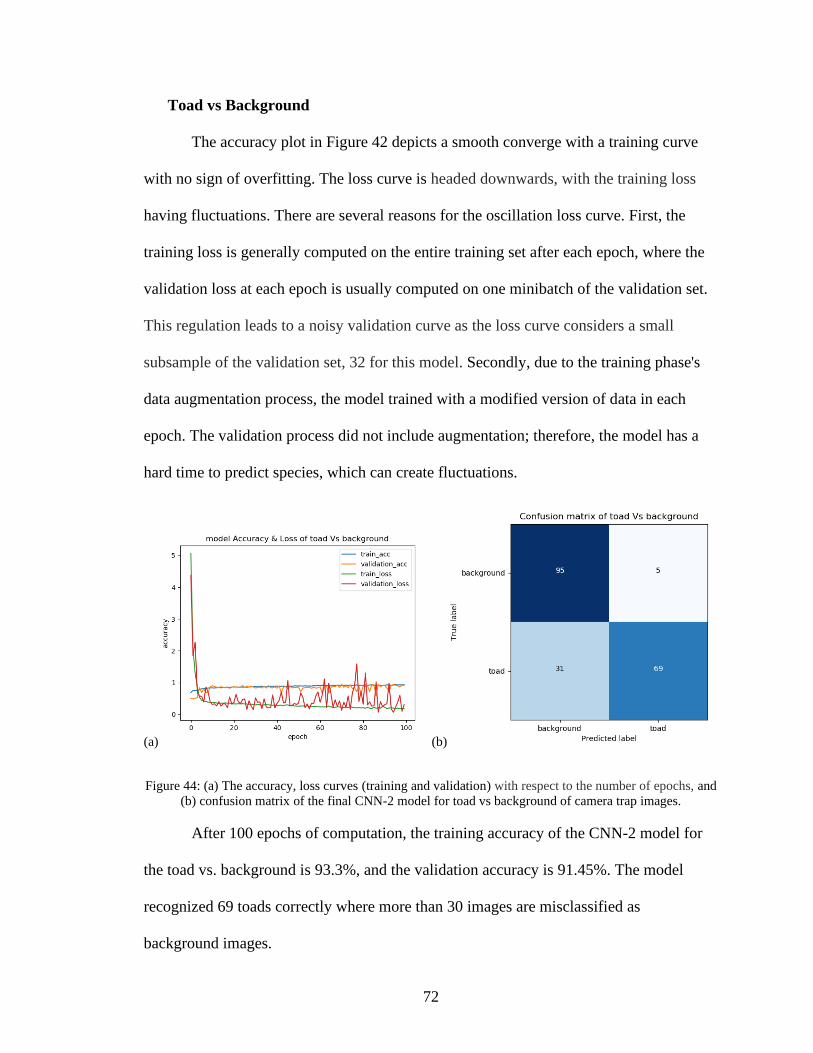
72
Toad vs Background
The accuracy plot in Figure 42 depicts a smooth converge with a training curve
with no sign of overfitting. The loss curve is headed downwards, with the training loss
having fluctuations. There are several reasons for the oscillation loss curve. First, the
training loss is generally computed on the entire training set after each epoch, where the
validation loss at each epoch is usually computed on one minibatch of the validation set.
This regulation leads to a noisy validation curve as the loss curve considers a small
subsample of the validation set, 32 for this model. Secondly, due to the training phase's
data augmentation process, the model trained with a modified version of data in each
epoch. The validation process did not include augmentation; therefore, the model has a
hard time to predict species, which can create fluctuations.
(a) (b)
Figure 44: (a) The accuracy, loss curves (training and validation) with respect to the number of epochs, and
(b) confusion matrix of the final CNN-2 model for toad vs background of camera trap images.
After 100 epochs of computation, the training accuracy of the CNN-2 model for
the toad vs. background is 93.3%, and the validation accuracy is 91.45%. The model
recognized 69 toads correctly where more than 30 images are misclassified as
background images.
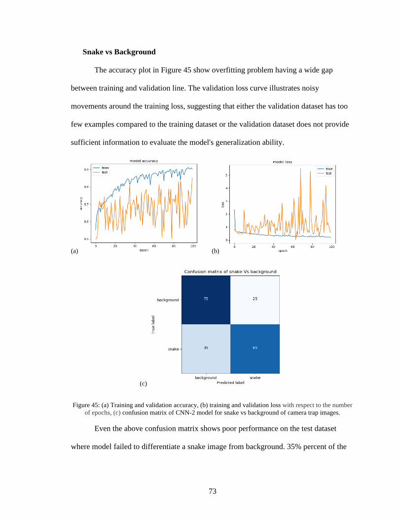
73
Snake vs Background
The accuracy plot in Figure 45 show overfitting problem having a wide gap
between training and validation line. The validation loss curve illustrates noisy
movements around the training loss, suggesting that either the validation dataset has too
few examples compared to the training dataset or the validation dataset does not provide
sufficient information to evaluate the model's generalization ability.
(a) (b)
(c)
Figure 45: (a) Training and validation accuracy, (b) training and validation loss with respect to the number
of epochs, (c) confusion matrix of CNN-2 model for snake vs background of camera trap images.
Even the above confusion matrix shows poor performance on the test dataset
where model failed to differentiate a snake image from background. 35% percent of the
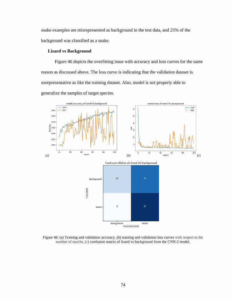
74
snake examples are misrepresented as background in the test data, and 25% of the
background was classified as a snake.
Lizard vs Background
Figure 46 depicts the overfitting issue with accuracy and loss curves for the same
reason as discussed above. The loss curve is indicating that the validation dataset is
unrepresentative as like the training dataset. Also, model is not properly able to
generalize the samples of target species.
(a) (b) (c)
Figure 46: (a) Training and validation accuracy, (b) training and validation loss curves with respect to the
number of epochs, (c) confusion matrix of lizard vs background from the CNN-2 model.
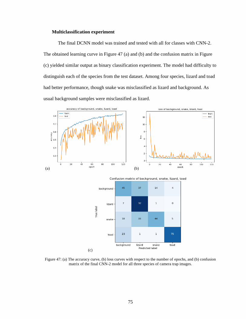
75
Multiclassification experiment
The final DCNN model was trained and tested with all for classes with CNN-2.
The obtained learning curve in Figure 47 (a) and (b) and the confusion matrix in Figure
(c) yielded similar output as binary classification experiment. The model had difficulty to
distinguish each of the species from the test dataset. Among four species, lizard and toad
had better performance, though snake was misclassified as lizard and background. As
usual background samples were misclassified as lizard.
(a) (b)
(c)
Figure 47: (a) The accuracy curve, (b) loss curves with respect to the number of epochs, and (b) confusion
matrix of the final CNN-2 model for all three species of camera trap images.
76
8.2.2.1 Attempts to Reduce Overfitting for CNN-2
The above result analysis depicted that the deep learning model performed better
on the training dataset than the test set due to the overfitting trend. Many experiments
have been carried out to minimize the overfitting phenomenon. The input image size,
filter size, number of neurons, learning rate, number of layers and dropout values were
systematically varied to understand their impact on classification accuracy. All the
CONV and dense layers were incorporated with a 0.5 Drop out value to avoid overfitting.
However, this regularization could not prevent the overfitting for CNN-2 models.
Moreover, EarlyStopping function has been adopted to mitigate the overfitting
issue. After trailing several regularization and hyper tuning process, only EarlyStopping
shows favorable outcome for lizard vs background and snake vs background experiment
as explained below.
Early Stopping
Lizard vs Background
The whole experimental process has repeated for 100 epochs to obtain reliable
results with a constant batch size of 32. However, the training process Figure 48
terminated at 60 epochs due to the use of callback function. The learning curve shows a
slightly better pattern. But no improvement in the validation accuracy has been observed
Surprisingly, the testing accuracy as in Figure 48 (c) has increased moderately from the
previous execution. The advantage of using callback function is to reach the same
accuracy within a smaller number of epochs, and computation time. The testing accuracy
has increased moderately from the previous execution.
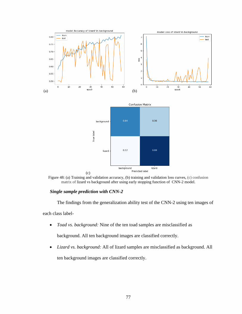
77
(a) (b)
(c)
Figure 48: (a) Training and validation accuracy, (b) training and validation loss curves, (c) confusion
matrix of lizard vs background after using early stopping function of CNN-2 model.
Single sample prediction with CNN-2
The findings from the generalization ability test of the CNN-2 using ten images of
each class label-
• Toad vs. background: Nine of the ten toad samples are misclassified as
background. All ten background images are classified correctly.
• Lizard vs. background: All of lizard samples are misclassified as background. All
ten background images are classified correctly.
78
• Snake vs. background: Seven of the ten snake images is detected correctly; three
samples are misclassified as background. Six of the background images are
misclassified as snake.
• Background vs. snake vs. lizard vs. toad: Two toad and five snake images have
recognized correctly.
In can be noticed that, data augmentation shows promises only for snake images,
where this method failed to improve recognition accuracy for lizard and toad. CNN-2
architecture predicted all the ten lizard samples, and 90% toad samples as background.
As expected, the model performed well for snake identification providing 70% positive
accuracy. However, this model also misclassified 60% background image as snake.
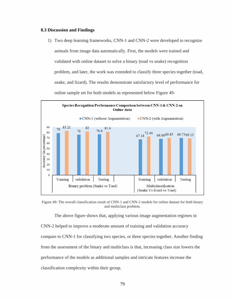
79
8.3 Discussion and Findings
1) Two deep learning frameworks, CNN-1 and CNN-2 were developed to recognize
animals from image data automatically. First, the models were trained and
validated with online dataset to solve a binary (toad vs snake) recognition
problem, and later, the work was extended to classify three species together (toad,
snake, and lizard). The results demonstrate satisfactory level of performance for
online sample set for both models as represented below Figure 49-
Figure 49: The overall classification result of CNN-1 and CNN-2 models for online dataset for both binary
and multiclass problem.
The above figure shows that, applying various image augmentation regimes in
CNN-2 helped to improve a moderate amount of training and validation accuracy
compare to CNN-1 for classifying two species, or three species together. Another finding
from the assessment of the binary and multiclass is that, increasing class size lowers the
performance of the models as additional samples and intricate features increase the
classification complexity within their group.
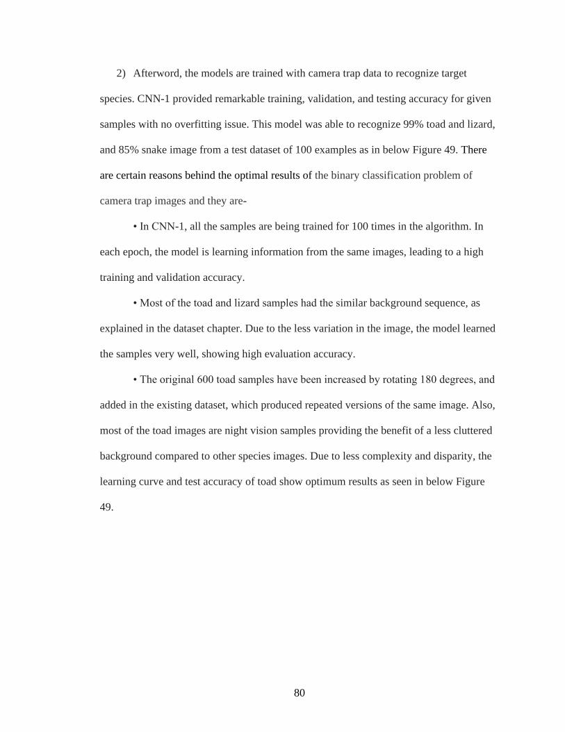
80
2) Afterword, the models are trained with camera trap data to recognize target
species. CNN-1 provided remarkable training, validation, and testing accuracy for given
samples with no overfitting issue. This model was able to recognize 99% toad and lizard,
and 85% snake image from a test dataset of 100 examples as in below Figure 49. There
are certain reasons behind the optimal results of the binary classification problem of
camera trap images and they are-
• In CNN-1, all the samples are being trained for 100 times in the algorithm. In
each epoch, the model is learning information from the same images, leading to a high
training and validation accuracy.
• Most of the toad and lizard samples had the similar background sequence, as
explained in the dataset chapter. Due to the less variation in the image, the model learned
the samples very well, showing high evaluation accuracy.
• The original 600 toad samples have been increased by rotating 180 degrees, and
added in the existing dataset, which produced repeated versions of the same image. Also,
most of the toad images are night vision samples providing the benefit of a less cluttered
background compared to other species images. Due to less complexity and disparity, the
learning curve and test accuracy of toad show optimum results as seen in below Figure
49.
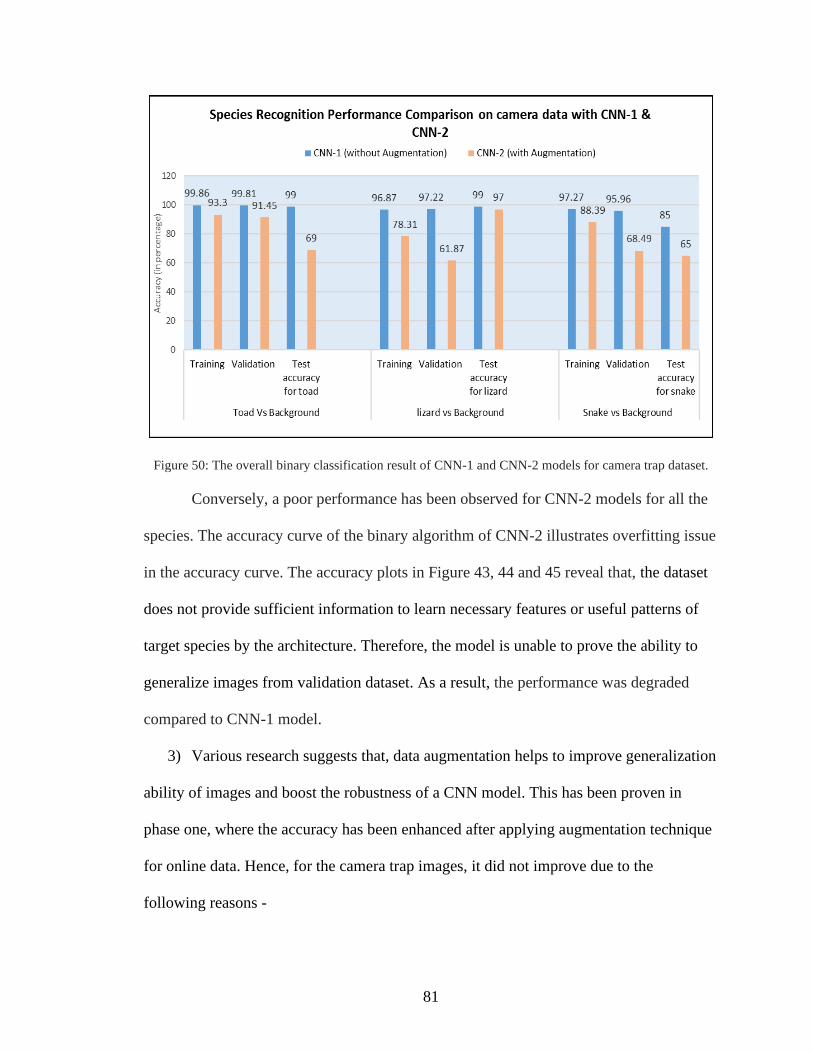
81
Figure 50: The overall binary classification result of CNN-1 and CNN-2 models for camera trap dataset.
Conversely, a poor performance has been observed for CNN-2 models for all the
species. The accuracy curve of the binary algorithm of CNN-2 illustrates overfitting issue
in the accuracy curve. The accuracy plots in Figure 43, 44 and 45 reveal that, the dataset
does not provide sufficient information to learn necessary features or useful patterns of
target species by the architecture. Therefore, the model is unable to prove the ability to
generalize images from validation dataset. As a result, the performance was degraded
compared to CNN-1 model.
3) Various research suggests that, data augmentation helps to improve generalization
ability of images and boost the robustness of a CNN model. This has been proven in
phase one, where the accuracy has been enhanced after applying augmentation technique
for online data. Hence, for the camera trap images, it did not improve due to the
following reasons -
82
(a) The CNN-2 models suffer from data deficiency. Moreover, in the dataset, the
samples have adjusted artificially to increase the dataset, eventually failed to
obtain the target class's feature.
(b) Due to the augmentation procedure, the model is training with a new set of
slightly modified data in each epoch. As the model sees a new set of transformed
images which is replacing the previous set, it is unable to learn the individual
meaningful pattern of species.
(c) Toad and lizard are too small to recognize with respect to the background
information. Moreover, the lizard and toad body shape, size, color have very high
similarity background properties.
(d) The snake images have advantages over other species with a considerable amount
of body size, shape, and diversity, which allow the algorithm to learn about the
distinct features and make them separate from a background image.
Also, it can be noted that, the generalization test has been done with 10 sample
per species. Conducting test process with more images might increase the prediction
accuracy for target species.
In conclusion, CNN-1 shows higher efficiency to predict camera trap data into
their label between the two models. Moreover, the advantage of CNN-1 is that it requires
less computation time and memory to train the dataset, while CNN-2 takes longer time to
compute as it generates a new set of augmented samples of the existing data in every
epoch for training purpose.
4) After several experiments it can be summarized that, a significant number of
83
imagery data, and a robust network can minimize the misclassification error providing a
good recognition accuracy. Also, an alternative labeling method such as ground truth
labeling can be investigated to teach the models about the complex features of species of
a challenging sample set.
5) To explore the potentiality of region based convolutional neural networks
(RCNN), a test has been conducted with the pre-trained ImageNet model: residual neural
network (ResNet). In this region-based object detection technique, the model tries to
identify the location of a target object of interest in an image, and then classify them to
obtain final object detections [76]. A pixel-based clustering algorithm is applied that
attempts to merge the similarities of color, texture, size, shape of object [76]. Afterward,
the model seeks a final meta-similarity to find a region of interest and then provides the
predicted score [76].
Some of the observations from the pre-trained ResNet model is included in
Appendix B. The pictures clearly reveal that, the ResNet neglected the target species in
the camera trap images and selected wrong objects location. Also, the model provided
incorrect prediction of the bounding box coordinates of the marked object location. The
reason is that ResNet is not trained with this particular data samples. The model needs to
train with camera trap dataset with appropriate labeling and annotaion of target species.
With proper training, the RCNN algorithm can be investigated in future for far more
accurate classification and object localization experiment.
84
9. CONCLUSION AND FUTURE WORK
The challenges associated with big data need to overcome with a structure that
will systematically and efficiently analyze information. A justified initial work of species
classification for phase one is presented with online images that depict potential success
for camera trap images. The experiment result demonstrates the feasibility of recognition
of animal species. Necessary changes have been made while training the original camera
trap images to reduce the effect of data imbalance and varying object position, lighting,
and weather condition challenges. However, real-world samples exhibit natural
adversarial prone, lowering the performance to recognize species from images. For
CNN-1, the average testing accuracy for toad and lizard is 99% and for snake is 85%
with respect to background examples. Nevertheless, in the generalization ability test from
a separate set of unlabeled data, this model recognizes 90% toad and lizard, and 100%
snake species from a set of ten images for each species. This results suggest that, for the
same background environment, CNN-1 model will be able to recognize species.
An alternative CNN architecture has been experimented to explore various
augmentation effects in the model by enhancing the amount of dataset and exploiting
specific properties. This process allows to train the model with a wide range of object
variations in form and shape. The binary classification experiment test accuracy of CNN-
2 for toad, snake and lizard is 69%, 65% and 25% consecutively with respect to the
background. In the generalization ability test, the training techniques with augmented
samples have a practical effect on a snake, adding no toad and lizard progress. In other
word, CNN-2 failed to distinguish lizards and toads from the background.
85
The results of CNN-2 validate that, the CNN framework will be able to recognize
the target species if the quality, and background view of the image belong to the similar
circumstance that have been provided for this project. Any changes in the target species
such as body size, shape, or the nature of presence of species in the surroundings, may
decline the recognition percentage. Both the models, (CNN-1) and (CNN-2) will perform
better in the classification process when objects or species have a decent presence in a
sample or have a pixelated value in the background.
Nevertheless, the above issues always will be a part of the problem in automatic
identification process with camera trap images. For snake identification, a sufficient
amount of data will enhance classification accuracy. The current models have substantial
room for improvement by making it more robust to detect challenging animal species
from the camera trap dataset. In order to determine the optimal recognition method,
further research is needed. Several deep learning architectures can be explored to find a
better recognition solution for three species, such as Region-based Convolutional Neural
Networks (RCNN), U-Net, and other deep learning networks.
86
APPENDIX SECTION
Appendix A
In an attempt to minimize overfitting and increase generalization ability in CNN-
2, several regularization techniques have been experimented in the architecture as
explained in section 8.2.2.1. The CNN-2 model was tested with a variety of combinations
of small learning rate and higher batch size that did not perform well in the validation and
test data. Also, a two-layer shallow model has been designed to ensure less complexity in
the model. Hence, the result was not improved. That is why the below two result has been
added in Appendix A.
Small Learning Rate and Higher Batch Size
An experiment was performed with a learning rate of 0.0001 and a batch size of
64 to minimize the overfitting effect in CNN-2. Still, the overfitting trend was not
improved from the previous one, as seen in Figure 51. The model predicted worst for the
testing sample set having background misclassification.
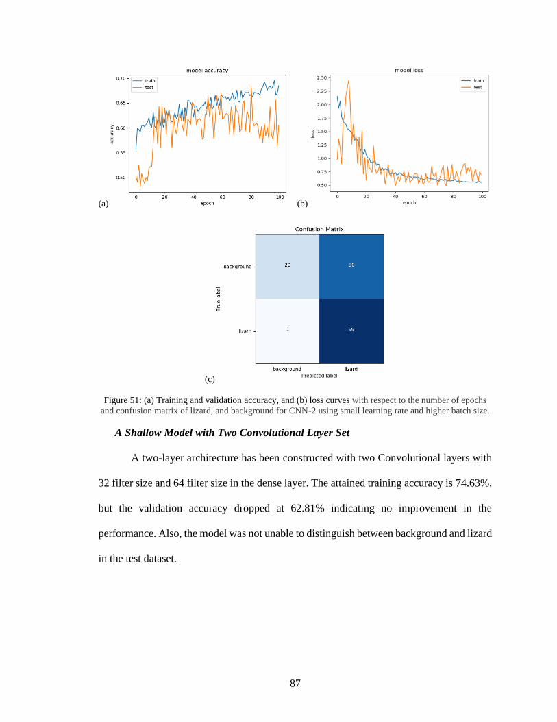
87
(a) (b)
(c)
Figure 51: (a) Training and validation accuracy, and (b) loss curves with respect to the number of epochs
and confusion matrix of lizard, and background for CNN-2 using small learning rate and higher batch size.
A Shallow Model with Two Convolutional Layer Set
A two-layer architecture has been constructed with two Convolutional layers with
32 filter size and 64 filter size in the dense layer. The attained training accuracy is 74.63%,
but the validation accuracy dropped at 62.81% indicating no improvement in the
performance. Also, the model was not unable to distinguish between background and lizard
in the test dataset.
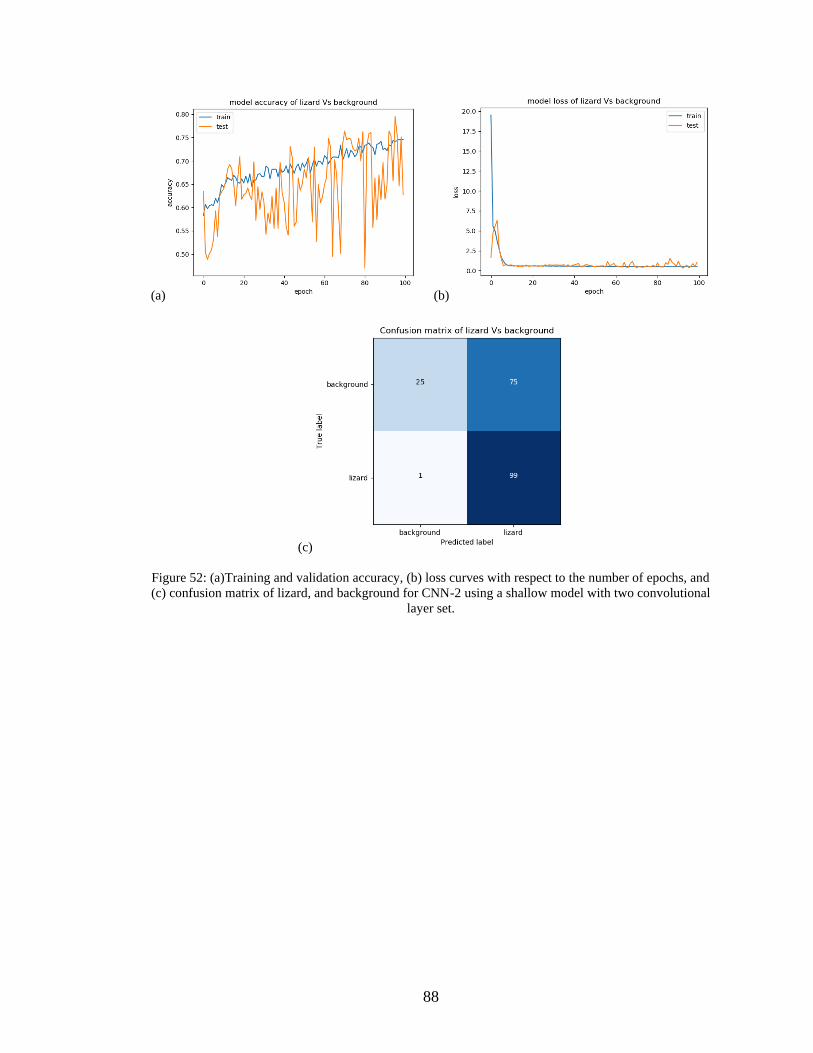
88
(a) (b)
(c)
Figure 52: (a)Training and validation accuracy, (b) loss curves with respect to the number of epochs, and
(c) confusion matrix of lizard, and background for CNN-2 using a shallow model with two convolutional
layer set.
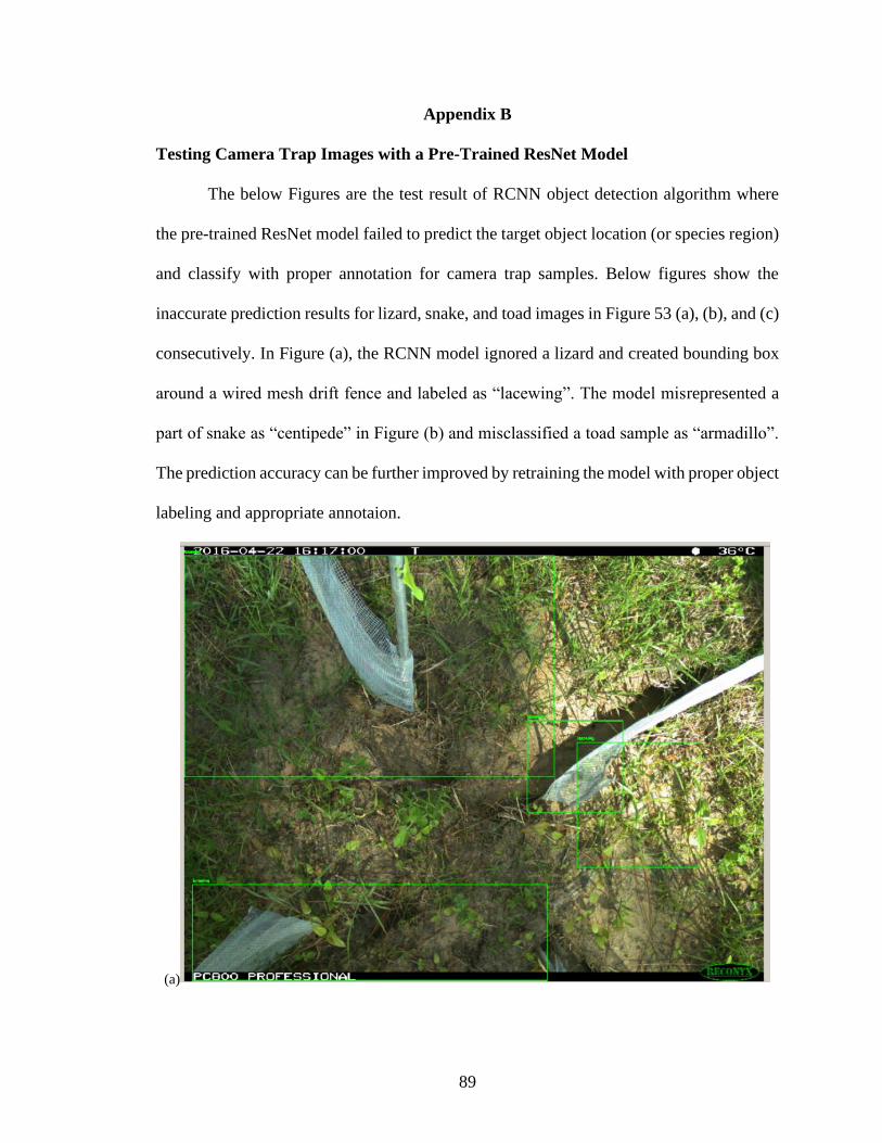
89
Appendix B
Testing Camera Trap Images with a Pre-Trained ResNet Model
The below Figures are the test result of RCNN object detection algorithm where
the pre-trained ResNet model failed to predict the target object location (or species region)
and classify with proper annotation for camera trap samples. Below figures show the
inaccurate prediction results for lizard, snake, and toad images in Figure 53 (a), (b), and (c)
consecutively. In Figure (a), the RCNN model ignored a lizard and created bounding box
around a wired mesh drift fence and labeled as “lacewing”. The model misrepresented a
part of snake as “centipede” in Figure (b) and misclassified a toad sample as “armadillo”.
The prediction accuracy can be further improved by retraining the model with proper object
labeling and appropriate annotaion.
(a)
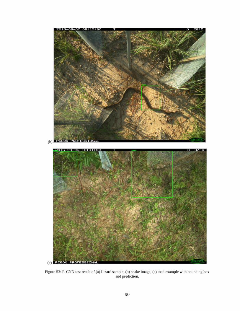
90
(b)
(c)
Figure 53: R-CNN test result of (a) Lizard sample, (b) snake image, (c) toad example with bounding box
and prediction.
91
REFERENCE
[1] J. W. Gibbons, D. E. Scott, T. J. Ryan, k. A. Buhlmann, T. D. Tuberville et al., “The global decline
of reptiles, déjà vu amphibians.”, Aug. 2000, Vol. 50 No. 8, BioScience 50:653-666.
[2] S. M. Whitfield, K. E. Bell, T. Philippi, M. Sasa, F. Bolaños, et al., “Amphibian and reptile declines
over 35 years at La Selva, Costa Rica”. Proceedings of the National Academy of Sciences of the
United States of America, 2007, vol. 104, no. 20, pp. 8352–8356, 2007,
doi: 10.1073/pnas.0611256104.
[3] M. Böhm, B. Collen, J. E. M. Baillie, P. Bowles, J. Chanson, et al., “The conservation status of the
world’s reptiles,” Biol. Conserv., vol. 157, pp. 372–385, 2013, doi: 10.1016/j.biocon.2012.07.015.
[4] L. D. Mech, S. M. Barber, “A critique of wildlife radio-tracking and its use in national parks.” Feb.
6, 2002, U.S. Geological Survey.
[5] G. Chen, T. X. Han, Z. He, R. Kays, and T. Forrester, “Deep Convolutional Neural Network Based
Species Recognition for Wild Animal Monitoring.” IEEE International Conference on Image
Processing (ICIP), 2014.
[6] C. Y. Yeo, S.A.R. Al-Haddad, C. K. Ng, “Animal Voice Recognition for Identification (ID)
Detection System”, 7th International Colloquium on Signal Processing and its Applications, 2011,
doi:10.1109/CSPA.2011.5759872.
[7] Z. He et al., “Visual Informatics Tools for Supporting Large-Scale Collaborative Wildlife
Monitoring with Citizen Scientists.” IEEE Circuits and Systems Mgazine, Feb. 12, 2016, doi:
10.1109/MCAS.2015.2510200.
[8] R. Kays, S. Tilak, B. Kranstauber, P. A. Jansen, C. Carbone, et al., “Monitoring wild animal
communities with arrays of motion sensitive camera traps”, Sep. 28,2010, arXiv:1009.5718v1.
[9] D. J. Welbourne, A. W. Claridge, D. J. Paull, and F. Ford, “Improving Terrestrial Squamate Surveys
with Camera-Trap Programming and Hardware Modifications,” Animals, vol. 9, no. 6, p. 388, Jun.
2019.
[10] D. J. Welbourne, D. J. Paull, A. W. Claridge, and F. Ford, “A frontier in the use of camera traps:
surveying terrestrial squamate assemblages,” Remote Sens. Ecol. Conserv., vol. 3, no. 3, pp. 133–
145, 2017, doi: 10.1002/rse2.57.
[11] A. C. Burton et al., “Wildlife camera trapping: A review and recommendations for linking surveys to
ecological processes,” J. Appl. Ecol., vol. 52, no. 3, pp. 675–685, 2015, doi: 10.1111/1365-
2664.12432.
[12] M. T. Hobbs and C. S. Brehme, “An improved camera trap for amphibians, reptiles, small mammals,
and large invertebrates,” PLoS One, vol. 12, no. 10, pp. 1–15, 2017,
doi: 10.1371/journal.pone.0185026.
[13] W. Zhang, J. Sun, and X. Tang, “From Tiger to Panda: Animal Head Detection,” IEEE Transactions
on Image Processing, vol. 20, no. 6, June 2011, doi: 10.1109/TIP.2010.2099126.
[14] R. Sahu, “Detecting and Counting Small Animal Species Using Drone Imagery by Applying Deep
Learning.” Visual Object Tracking in the Deep Neural Networks Era, Aug. 09, 2019,
doi- 10.5772/intechopen.88437.

92
[15] A. Gómez, A. Salazar, and F. Vargas, “Towards automatic wild animal monitoring: Identification of
animal species in camera-trap images using very deep convolutional neural networks,” Mar. 22
2016, doi: arXiv:1603.06169, 2016.
[16] S. Schneider, G. W. Taylor, S. C. Kremer, “Deep Learning Object Detection Methods for Ecological
Camera Trap Data.” 15th Conference on Computer and Robot Vision, 2018,
doi: 10.1109/CRV.2018.00052.
[17] A. Rosebrock, Deep Learning for Computer Vision with Python, ImageNet Bundle. 1st Edition,
PYIMAGESEARCH, 2017.
[18] “Image Data Pre-Processing for Neural Networks.” [Online]. Available:
https://becominghuman.ai/image-data-pre-processing-for-neuralnetworks-498289068258
[Accessed: 20-Dec-2019].
[19] A. W. Ferguson, M. M. McDonough, and M. R. J. Forstner, “Herpetofaunal inventory of camp
mabry, Austin, Texas: Community composition in an urban landscape,” Texas Journal of Science,
vol. 60, no. 2. pp. 123–136, 2008.
[20] M. A. Gaston, A. Fuji, F. W. Weckerly, and M. R. J. Forstner, “Potential component allee effects
and their impact on wetland management in the conservation of endangered anurans,” PLoS One,
vol. 5, no. 4, 2010, doi: 10.1371/journal.pone.0010102.
[21] D. J. Brown, A. Duarte, I. Mali, M. C. Jones, M. R.J. Forstner, “Potential impacts of a high severity
wildfire on abundance, movement, and diversity of Herpetofauna in the lost pines ecoregion of
Texas”, Herpetological Conservation and Biology, July 2014.
[22] A. A. Bashit and D. Valles, “A Mel-Filterbank and MFCC-based Neural Network Approach to Train
the Houston Toad Call Detection System Design,” IEEE 9th Annual Information Technology,
Electronics and Mobile Communication Conference (IEMCON), 2018, pp. 438–443.
[23] A. A. Bashit and D. Valles, “MFCC-based Houston Toad Call Detection using LSTM,” The
International Symposium on Measurement, Control, and Robotics (ISMCR 2019), Houston, Texas,
September 2019
[24] L. A. Fitzgerald, D. Walkup, K. Chyn, E. Buchholtz, N. Angeli, and M. Parker, The future for
reptiles: Advances and challenges in the anthropocene, vol. 1–5, no. December. Elsevier Inc., 2017.
[25] C. S. Adams, W. A. Ryberg, T. J. Hibbitts, B. L. Pierce, J. B. Pierce, and D. C. Rudolph,
“Evaluating effectiveness and cost of time-lapse triggered camera trapping techniques to detect
terrestrial squamate diversity,” Herpetol. Rev., vol. 48, no. 1, pp. 44–48, 2017, [Online]. Available:
https://www.fs.usda.gov/treesearch/pubs/53958.
[26] M. Willi, R. T. Pitman, A. W. Cardoso, C. Locke, A. Swanson, et al. “Identifying animal species in
camera trap images using deep learning and citizen science”, 2017, IEEE International Conference
on Data Science and Advanced Analytics (DSAA), doi: 10.1111/2041-210X.13099.
[27] “Zooniverse Database: Popular platform for people-powered research.” [Online]. Available:
https://www.zooniverse.org/about, [Accessed: 29-Dec-2020].
[28] J. Wäldchen and P. Mäder, “Machine learning for image based species identification,” Methods in
Ecology and Evolution, vol. 9, no. 11, pp. 2216–2225, 2018, doi: 10.1111/2041-210X.13075.
[29] H. Nguyen, S. J. Maclagan, T. D. Nguyen, T. Nguyen, P. Flemons, et al. “Animal Recognition and
Identification with Deep Convolutional Neural Networks for Automated Wildlife Monitoring”,
2017, International Conference on Data Science and Advanced Analytics.
93
[30] J. Brownlee, “Introduction to the ImageNet Challenge (ILSVRC)” [Online]. Available:
https://machinelearningmastery.com/introduction-to-the-imagenet-large-scale-visual-recognition-
challenge-ilsvrc/ [Accessed: 2-Feb-2020].
[31] “ImageNet Large Scale Visual Recognition Challenge (ILSVRC) annual competition.” [Online].
Available:http://image-net.org/challenges/LSVRC/ [Accessed: 29-Dec-2020].
[32] X. Yu, J. Wang, R. Kays, P. Jansen, T. Wang, and T. Huang, “Automated identification of animal
species in camera trap images,” EURASIP J. Image Video Process., vol. 1, pp. 1–10, 2013.
[33] A. Rosebrock, Deep Learning for Computer Vision with Python. 1st Edition, PYIMAGESEARCH,
2017.
[34] J. Wang, J. Yang, K. Yu, F. Lv, T. Huang, and Y. Gong, “Locality-constrained linear coding for
image classification,” Proc. IEEE Comput. Soc. Conf. Comput. Vis. Pattern Recognit., pp. 3360–
3367, 2010, doi: 10.1109/CVPR.2010.5540018.
[35] J. Yang, K. Yu, Y. Gong and T. Huang, "Linear spatial pyramid matching using sparse coding for
image classification," IEEE Conference on Computer Vision and Pattern Recognition, Miami, FL,
2009, pp. 1794-1801, doi: 10.1109/CVPR.2009.5206757.
[36] M. S. Norouzzadeh, A. Nguyen, M. Kosmala, A. Swanson, M. Palmer, C. Packer, and J. Clune,
“Automatically identifying, counting, and describing wild animals in camera-trap images with deep
learning,”. ArXiv:1703.05830v5, 2017.
[37] M. A. Tabak et al., “Machine learning to classify animal species in camera trap images: Applications
in ecology,” Methods in Ecology and Evolution, vol. 10, no. 4, pp. 585–590, 2019, doi:
10.1111/2041-210X.13120.
[38] R. Chen, R. Little, L. Mihaylova, R. Delahay, and R. Cox, “Wildlife surveillance using deep
learning methods,” Ecology and Evolution, vol. 9, no. 17, pp. 9453–9466, 2019, doi:
10.1002/ece3.5410.
[39] O. Russakovsky, J. Deng, H. Su, J. Krause, S. Satheesh, et al., “ImageNet Large Scale Visual
Recognition Challenge,” International Journal of Computer Vision, vol. 115, no. 3, pp. 211–252,
2015, doi: 10.1007/s11263-015-0816-y.
[40] “How to build a data set for machine learning project.” [Online]. Available:
https://towardsdatascience.com/how-to-build-a-data-set-for-your-machine-learning-project-
5b3b871881ac. [Accessed: 27-Oct-2020].
[41] “CalPhotos: A database of photos of plants, animals, habitats and other natural history subjects [web
application]. BSCIT, University of California, Berkeley.” [Online]. Available:
https://calphotos.berkeley.edu/. [Accessed: 10-Oct-2020].
[42] “OpenImages: A public dataset for large-scale multi-label and multi-class image classification,
2017.” [Online]. Available: https://storage.googleapis.com/openimages/web/index.html. [Accessed:
10-Sept-2020].
[43] Griffin, G. Holub, AD. Perona, “The Caltech 256.: Caltech Technical Report. [Online]. Available:
http://www.vision.caltech.edu/Image_Datasets/Caltech256/ [Accessed: 10-Nov-2019].
[44] “Pixabay: Open sourced free image database.” [Online]. Available:
https://pixabay.com/images/search/. [Accessed: 30-Sept-2020].
94
[45] “What are the Bing Search APIs.” [Online]. Available: https://docs.microsoft.com/en-
us/azure/cognitive-services/bing-web-search/bing-api-comparison [Accessed: 10-Sept-2020].
[46] “Artificial Intelligence vs. Machine Learning vs. Deep Learning: What’s the Difference.” [Online].
Available: https://medium.com/ai-in-plain-english/artificial-intelligence-vs-machine-learning-vs-
deep-learning-whats-the-difference-dccce18efe7f. [Accessed: 30-Oct-2020].
[47] “AI vs Machine Learning vs Deep Learning: What's the Difference?”[Online]. Available:
https://www.guru99.com/machine-learning-vs-deep-learning.html#1 [Accessed: 30-Oct-2020].
[48] “A Basic Introduction To Neural Networks.” [Online]. Available:
http://pages.cs.wisc.edu/~bolo/shipyard/neural/local.html [Accessed: 30-Oct-2020].
[49] “Convolutional Neural Networks for Visual Recognition.” [Online]. Available:
https://cs231n.github.io/neural-networks-1/ [Accessed: 30-Oct-2020].
[50] A. Géron, Hands-On Machine Learning with Scikit-Learn & TensorFlow. March 2017, Published by
O’Reilly Media, Inc., 1005 Gravenstein Highway North, Sebastopol, CA 95472. doi: 978-1-491-
96229-9.
[51] S. Hijazi, R. Kumar, and C. Rowen. “Using Convolutional Neural Networks for Image
Recognition.” IP Group, Cadence, 2015
[52] N. O’Mahony et al., “Deep Learning vs. Traditional Computer Vision,” Computer Vision
Conference (CVC), vol. 943, no. Cv, pp. 128–144, 2020, doi: 10.1007/978-3-030-17795-9_10.
[53] “How Do Convolutional Layers Work in Deep Learning Neural Networks?” [Online]. Available:
https://machinelearningmastery.com/convolutional-layers-for-deep-learning-neural-networks/.
[Accessed: 27-Oct-2020].
[54] “The Computer Vision Pipeline, Part 4: feature extraction.” [Online]. Available:
https://freecontent.manning.com/the-computer-vision-pipeline-part-4-feature-extraction/. [Accessed:
27-Oct-2020].
[55] “Perceptrons | Using neural nets to recognize handwritten digits | CHAPTER 1”[Online]. Available:
http://neuralnetworksanddeeplearning.com/chap1.html. [Accessed: 27-Oct-2020].
[56] S. Raschka and V. Mirjalili, 2017. Python Machine Learning - Second Edition. Birmingham: Packt
Publishing.
[57] “Handling Imbalanced Datasets in Deep Learning.” [Online]. Available:
https://towardsdatascience.com/handling-imbalanced-datasets-in-deep-learning-f48407a0e758.
[Accessed: 27-Oct-2020].
[58] “Data Augmentation techniques in python.” [Online]. Available:
https://towardsdatascience.com/data-augmentation-techniques-in-python-f216ef5eed69. [Accessed:
27-Oct-2020].
[59] “Keras ImageDataGenerator and Data Augmentation.” [Online]. Available:
https://www.pyimagesearch.com/2019/07/08/keras-imagedatagenerator-and-data-augmentation/.
[Accessed: 27-Oct-2020].
[60] “Improving Performance of Convolutional Neural Network!” [Online]. Available:
https://medium.com/@dipti.rohan.pawar/improving-performance-of-convolutional-neural-network-
2ecfe0207de7. [Accessed: 27-Oct-2020].
95
[61] R. Yamashita, M. Nishio, R. K. G. Do, and K. Togashi, “Convolutional neural networks: an
overview and application in radiology,” Insights Imaging, vol. 9, no. 4, pp. 611–629, 2018, doi:
10.1007/s13244-018-0639-9.
[62] Z. Reitermanov, “Data Splitting,” pp. 31–36, WDS'10 Proceedings of Contributed Papers, 2010,
doi: ISBN 978-80-7378-139-2 © MATFYZPRESS.
[63] “Exploring Data Augmentation with Keras and TensorFlow.” [Online]. Available:
https://towardsdatascience.com/exploring-image-data-augmentation-with-keras-and-tensorflow-
a8162d89b844. [Accessed: 27-Oct-2020].
[64] “An intuitive guide to Convolutional Neural Networks.” [Online]. Available:
https://www.freecodecamp.org/news/an-intuitive-guide-to-convolutional-neural-networks-
260c2de0a050/. [Accessed: 17-Oct-2020].
[65] M. I. U. Haque, “A Facial Expression Recognition Application Development Using Deep
Convolutional Neural Network For Children With Autism Spectrum Disorder To Help Identify
Human Emotions,” Aug. 2019, Accessed: Nov. 05, 2020. [Online]. Available:
https://digital.library.txstate.edu/handle/10877/8457.
[66] “A Gentle Introduction to Batch Normalization for Deep Neural Networks.” [Online]. Available:
https://machinelearningmastery.com/batch-normalization-for-training-of-deep-neural-networks/.
[Accessed: 27-Oct-2020].
[67] A. Sunil, “arjun921/Indian-Snakes-Dataset: Initial Release (Version v1.0.0). Zenodo, (2020,
November 10).” [Online]. Available: http://doi.org/10.5281/zenodo.4266398. [Accessed: 02-Sep-
2019].
[68] A. Duong, “Introduction to callbacks in Keras.” [Online]. Available:
https://www.kdnuggets.com/2019/08/keras-callbacks-explained-three minutes.html.
[Accessed: 27-Oct-2020].
[69] “How to Improve a Neural Network With Regularization.” [Online]. Available:
https://towardsdatascience.com/how-to-improve-a-neural-network-with-regularization-
8a18ecda9fe3. [Accessed: 27-Oct-2020].
[70] S. B. Islam, D. Valles, “Identification of Wild Species in Texas from Camera-trap Images using
Deep Neural Network for Conservation Monitoring”, 10th Annual Computing and Communication
Workshop and Conference (CCWC), 2020, ISBN: 978-1-7281-3782-7.
[71] “Image data preprocessing | Keras.” [Online]. Available:
https://keras.io/api/preprocessing/image/#flow_from_directory. [Accessed: 31-Oct-2020].
[72] “Difference Between a Batch and an Epoch in a Neural Network” [Online]. Available:
https://machinelearningmastery.com/difference-between-a-batch-and-an-epoch/. [Accessed: 05-Oct-
2020].
[73] “LEAP - High Performance Computing Cluster, Texas State University” [Online]. Available:
https://doit.txstate.edu/rc/leap.html, [Accessed: 27-Nov-2020].
[74] “Stride | Convolutional Neural Networks cheatsheet”. [Online]. Available:
https://stanford.edu/~shervine/teaching/cs-230/cheatsheet-convolutional-neural-networks.
[Accessed: 27-Oct-2020].
96
[75] “Unsplash: Open sourced free image database”. [Online]. Available: https://unsplash.com/
[Accessed: 27-Oct-2020].
[76] I. S. Abdurrazaq, S. Suyanto, and D. Q. Utama, “Image-Based Classification of Snake Species Using
Convolutional Neural Network,” 2019 2nd Int. Semin. Res. Inf. Technol. Intell. Syst. ISRITI 2019,
pp. 97–102, 2019, doi: 10.1109/ISRITI48646.2019.9034633.
[77] A. Patel, L. Cheung, N. Khatod, I. Matijosaitiene, A. Arteaga, and J. W. Gilkey, “Revealing the
unknown: Real-time recognition of galápagos snake species using deep learning,” Animals, vol. 10,
no. 5, 2020, doi: 10.3390/ani10050806.
[78] L. Bloch et al., “Combination of image and location information for snake species identification
using object detection and EfficientNets Combination of image and location information for snake
species identification using object detection and EfficientNets FHDO Biomedical,” Conf. Labs Eval.
Forum, vol. 2696, no. September, 2020, [Online]. Available: http://ceur-ws.org/Vol-
2696/paper_201.pdf.


