ec1 e-companion to Rahmandad and Sterman: Heterogeneity and Network Structure in the Dynamics of Diffusion: Comparing Agent-Based and Differential Equation Models
1
Supplementary material to accompany:
Heterogeneity and Network Structure in the Dynamics of Diffusion: Comparing Agent-Based and Differential Equation Models
Hazhir Rahmandad [email protected], John Sterman [email protected]

ec2 e-companion to Rahmandad and Sterman: Heterogeneity and Network Structure in the Dynamics of Diffusion: Comparing Agent-Based and Differential Equation Models
This supplement documents the DE and AB models and results, including the construction of
the different networks for the AB simulations, sensitivity analysis, the calibration process and
results, and instructions for simulating the model and replicating the results. The model, imple-
mented in the Anylogic simulation environment, is available at:
http://web.mit.edu/hazhir/www/research.html
EC.1. Formulation for the Agent-Based SEIR Model
We develop the agent based SEIR model and derive the classical differential equation model
from it. Figure EC.1 shows the state transition chart for individual j. Individuals progress from
Susceptible to Exposed (asymptomatic infectious) to Infectious (symptomatic) to Recovered (im-
mune to reinfection). In the classical epidemiology literature the recovered state is often termed
“Removed” to denote both recovery and cumulative mortality.
S[j]Susceptible
E[j]Exposed
I[j]Infectious
R[j]
Recoveredf[j]
InfectionRate
e[j]Emergence
Rate
r[j]
RecoveryRate
Figure EC.1 State Transitions for the AB SEIR model
The states SEIR are mutually exclusive; each individual in the AB model can only be in one
of the states. We first derive the individual Infection Rate f[k] (the hazard of infection for a sus-
ceptible individual), then the Emergence and Recovery Rates e[j] and r[j] for individuals in the
exposed and infectious states.
Infection Rate: For infection to occur Susceptible individuals must come into contact with
either an Infectious or Exposed individual. Some of these contacts result in transmission of the
infection. Infection (the transition from S to E) for susceptible individual k occurs if, first, the
individual comes into contact with an individual j in either the E or I state, and second, that con-
tact results in transmission of the infectious agent. The probability of contact between individual
j and k in a short interval of time, dt, is denoted Cdt[j,k]. The probability of transmission from j
to k given such a contact (infectivity) is denoted ij.
ec3 e-companion to Rahmandad and Sterman: Heterogeneity and Network Structure in the Dynamics of Diffusion: Comparing Agent-Based and Differential Equation Models
Contacts between individuals occur with probabilities conditioned by the network of rela-
tionships in the population. Assuming contacts within the relationship network are independent
events, the expected individual Infection Rate, f[k], can be found by summing the probabilities
of contact with each individual in states E and I and finding the infectious contact hazard by tak-
ing the limit of the sum of infectious contact probabilities as the time interval dt approaches zero:
f[k]= dtikjCdt EorIj
jdt /)],[(0
lim!"
#$
= ))/)],[((0
lim( dtikjCdtEorIj
jdt!"
#$
= ]),[( kjZEorIj
!"
(EC.1)
In the following section we find the expected infectious contact rate between individuals j
and k, Z[j,k], by deriving the formulations for its components based on the implementation of the
AB model in the paper.
In the agent-based model, contacts between each E or I individual and other individuals in
the population occur through the network of relationships between them. Infection can only oc-
cur when these contacts are with an individual in state S. Therefore, Cdt[j,k] is composed of two
components: (1) The event that an individual j in the state E or I (Rdt,n[j]) has (n) contact(s),
within dt, and (2) The probability that any of these (n) contacts is with individual k in the state S
(P[j,k]):
)])kP[j,-(1-(1[j]R k][j,C n
1n ndt,dt !"
=#= (EC.2)
Contacts for an E or I individual are assumed independent random variables with stationary
increments and therefore have a Poisson distribution with parameter L[j]:
!
Rdt,n[ j] =(L[ j] " dt)
n" e
(#L[ j ]"dt )
n! (EC.3)
!
L[ j] = c j "H[ j] (EC.4)
where cj, the base contact rate, equals cIS or cES depending on whether individual j is in the E
or I state, and H[j] is the heterogeneity factor for individual j (defined below).
When contact occurs, the probability individual j contacts an individual selected randomly
from the N-1 others is:

ec4 e-companion to Rahmandad and Sterman: Heterogeneity and Network Structure in the Dynamics of Diffusion: Comparing Agent-Based and Differential Equation Models
Probability(j contacting k| j has a contact)= P[j,k]= !"
#
#
Ni
iKjiNWi
kKjkNWk$
$
%
%
][/],[][
][/],[][ (EC.5)
where:
λ[j]: The individual heterogeneity factor. Set to 1 in the homogeneous scenarios. In the hetero-
geneous cases λ[j] is drawn from a uniform distribution U[0.25-1.75].
K[j]: The number of links individual j has in his or her network.
NW[i,j], the network link, is 1 if there is a link between individuals i and j and 0 if there is none,
or if i=j. N is the set of all individuals in the population.
The parameter τ captures the time constraint on contacts. In the homogeneous scenarios τ =
1. The total time for contacts with others is fixed, so that individuals with more links have fewer
chances of contact with each link, compensating for the heterogeneity created by differing degree
distributions in different networks. In the heterogeneous scenarios τ = 0 so that the probability of
contact through all links is constant: those with more links contact more people (on average).
The formulation ensures that contacts of the E or I individuals are distributed among other
population members depending on their heterogeneity factor and their connectedness.
The overall heterogeneity factor for individual j, H[j], is defined to ensure (1) that contact
frequencies capture heterogeneity among individuals, represented by λ[j]; (2) that individual
contact frequencies depend on the number of links to each individual in the heterogeneous condi-
tion but are independent of link density in the homogeneous condition; and (3) that the mean
contact frequency across the entire population remains (in expectation) equal to that in the differ-
ential equation model. Note that this formulation captures two types of heterogeneity. First, in-
dividual-level heterogeneity is captured through λ[j]: people with higher λ will have higher con-
tact rates. Second, network-level heterogeneity considers how many connections an individual
has and therefore how likely it is for that person to contact any of those connections. Conse-
quently:
NWjK
NjWjjH
!
!!=
"
#
][
][][][ (EC.6)
where:

ec5 e-companion to Rahmandad and Sterman: Heterogeneity and Network Structure in the Dynamics of Diffusion: Comparing Agent-Based and Differential Equation Models
W[j] is the weighted sum of links to individual j:
!"
#Ni
iKjiNWi$% ][/],[][ , (EC.7)
and WN, the population level weighted sum of W, normalizes H[j] so that the expected value of
mean contacts equals the value in the DE model.
Hence
WN =
!
"[i] #W [i]
K[i]$
N
% . (EC.8)
Finally, ij, the probability of transmission given a contact between infectious individual j and
susceptible k equals iES or iIS depending on whether individual j is in the E or I state.
Therefore we can find the infectious contact rate between an individual k in state S and indi-
vidual j in state E or I, Z[j,k], by substituting its components. Specifically, from eq. EC.1,
Z[j,k] is defined as ))/],[((0
limdtikjC
dtjdt !
"
and from eq. EC.2 we have )])kP[j,-(1-(1[j]R k][j,C n
1n ndt,dt !"
=#= , giving
Z[j,k] = )/)],[((0
limdtikjC
dtjdt !
"= )/))])kP[j,-(1-(1[j]R((
0
limn
1n ndt, dtidt
j!!"
#$
=. (EC.9)
Substituting R[j] , P[j,k] and their components from equations EC.3-EC.8, we find Z[j,k] in
terms of the model parameters and variables (individual contact rates, infectivities, heterogeneity
factors, and network structure),
Z[j,k] = jj
li
ickKjK
kjkjNW
lKiK
liliNW
N!!
!
!!
""""
#
$
%%%%
&
'
!
!!(
)
)
**** ])[][(
][][],[
])[][(
][][],[
,
(EC.10)
yielding the infection hazard for individual k in the state S:
!
f [k] = Z[ j,k]
j"E , I
# . (EC.11)

ec6 e-companion to Rahmandad and Sterman: Heterogeneity and Network Structure in the Dynamics of Diffusion: Comparing Agent-Based and Differential Equation Models
Emergence and Recovery: The DE SEIR model assumes populations within each state are well
mixed. Consider the recovery process (emergence is analogous). Perfect mixing implies that the
hazard rate of recovery for an infectious individual (the transition from I to R) depends only on
the expected duration of the infectious phase, 1/δ, and is independent of how long that particular
individual has been in the I state. Consequently residence times for infectious individuals are
distributed exponentially. In the AB model, the duration of the infectious stage for infectious
individual j is randomly drawn from the exponential distribution with mean duration 1/δ. Hence
the hazard rate for recovery is r[j] = δ. Emergence (the transition from E to I) is formulated
analogously, so e[j] = ε, where ε is the hazard rate for emergence.
EC.2. Deriving the deterministic compartment (differential equation) model
Figure EC.2 shows the structure of the deterministic compartment DE model.
Figure EC.2 The structure of the SEIR differential equation model.

ec7 e-companion to Rahmandad and Sterman: Heterogeneity and Network Structure in the Dynamics of Diffusion: Comparing Agent-Based and Differential Equation Models
The deterministic compartment model can be derived from the underlying stochastic agent-
based model by assuming (1) homogeneity of all individuals; (2) perfect mixing within com-
partments; and (3) the rates for the DE model are equated with the infinitesimal transition rate of
the underlying stochastic transmission model.
To derive the DE formulation for the infection rate, fDE, sum the individual infection rates
f[j]:
fDE =!J
f[j]= !!J K
Z[j,k]. (EC.12)
Homogeneity implies all individuals have the same number of links, K[j] = K[k] = K, and the
same propensity to use their links, λ[j] = λ[k] = 1. Therefore:
!
"""=
jk
jj
kjNW
kjNWNickjZ
,
],[
],[],[ . (EC.13)
NW[j,k] depends on the network structure. However, in the DE model individuals are assumed
to be well mixed, implying everyone is linked to everyone else. Therefore
NW[j,k]/ !jk ,
NW[j,k]=1/|N|2 (EC.14)
yielding
N
ickjZ
jj !=],[ . (EC.15)
Noting that homogeneity implies contact frequencies and infectivities are equal within states
(cj = cES and ij = iES for all E and cIS and ij = iIS for all I) and substituting into the equation for the
infection rate yields:
fDE = ! !!! !" """ #"
+=Sk Ij
ISIS
Ej
ESES
Sk IEj
jjicic
NN
ic)..(
1. (EC.16)
which simplifies into the formulation for the infection rate in the DE model:
fDE = (cES··iES·|E| + cIS·iIS·|I|) · (|S|/|N|). (EC.17)

ec8 e-companion to Rahmandad and Sterman: Heterogeneity and Network Structure in the Dynamics of Diffusion: Comparing Agent-Based and Differential Equation Models
The aggregate emergence and recovery rates in the DE are the sum of the expected individual
emergence and recovery rates:
!
eDE = E(e[ j])j"E
# = $ = E $j"E
# and
!
rDE = E(r[ j])j"I
# = $ = I$j"I
# (EC.18)
which is the formulation for a first-order exponential delay with hazard rates ε and
δ, respectively. The full SEIR model is thus:1
fdt
dS!= , ef
dt
dE!= , re
dt
dI!= (EC.19)
f= (cES·iES·E + cIS·iIS·I)(S/N) (EC.20)
!
e = "E (EC.21)
!
r = "I (EC.22)
EC.3. Network Structure
The connected and lattice networks are deterministic and hence the same in each AB simula-
tion. The random, scale free, and small world networks are stochastic. Each AB simulation of
these networks uses a different realization drawn from the appropriate network distribution. We
assume, for each realization, a fixed network (FN) model: the structure of each network remains
unchanged over the time horizon of the simulations. Moving from an FN to dynamic network in
which arcs among nodes change over the time horizon of the epidemic, either exogenously or
endogenously, would introduce additional mixing. The details of construction for each network
follow.
Connected: every node is connected to every other node.
1 Note that in the derivation of the individual-level AB model, the symbols S, E, I and R denote the sets of individu-als in the susceptible, exposed, infectious and removed states, respectively (with, e.g., |E| denoting the number of exposed individuals in the set E, while, consistent with standard practice, in the DE model (eq. 19-22), S, E, I and R are continuous, real-valued state variables representing the number of people in each state rather than the set of indi-viduals in each state.

ec9 e-companion to Rahmandad and Sterman: Heterogeneity and Network Structure in the Dynamics of Diffusion: Comparing Agent-Based and Differential Equation Models
Random: The probability of a connection between nodes i and j is fixed, p=k/(N-1), where k is
the average number of links per person. In the base case k = 10 and N = 200. In the sensitivity
analysis over population size, k = 6 and 18 when N = 50 and 800, respectively.
Scale-free: Barabasi and Albert (1999) outline the preferential attachment algorithm to grow
scale-free networks. The algorithm starts with m0 initial nodes and adds new nodes one at a time.
Each new node is connected to previous nodes through m new links, where the probability each
existing node j receives one of the new links is m*K[j]//ΣK[j] where K[j] is the number of links
into node j. The probability that node j has connectivity smaller than k after t time steps is then:
P(K[j]t<k) = 1 – m2t/(k2(t + m0)) (EC.23)
We use the same procedure with m = m0 = k (the average number of links per person). Fol-
lowing the original paper (Albert 2005, personal communication), we start with m0 individuals
connected to each other in a ring, and then add the rest of the N – m0 individuals to the structure.
The model accompanying the online material includes the Java code used to implement all net-
works.
Small World: Following Watts and Strogatz (1998), we build the small world network by or-
dering all individuals into a one-dimensional ring lattice in which each individual is connected to
the k/2 closest neighbors. Then we rewire these links to a randomly chosen member of the popu-
lation with probability p = 0.05
Ring Lattice: In the ring lattice each node is linked to the k/2 nearest neighbors on each side of
the node (equivalent to the small world case with zero probability of long-range links.) EC.4. Histogram of Final Size for each network and heterogeneity condition
Histograms for the fraction of the population ultimately infected (final size, F) are shown in
Figure EC.3 for each network and heterogeneity condition. The heterogeneous cases are shown
in blue and homogeneous cases in red.

ec10 e-companion to Rahmandad and Sterman: Heterogeneity and Network Structure in the Dynamics of Diffusion: Comparing Agent-Based and Differential Equation Models
0
10
20
30
40
50
60
0.00
0.08
0.16
0.24
0.32
0.40
0.48
0.56
0.64
0.72
0.80
0.88
0.96
Connected Network
Pe
rce
nta
ge
Final Size
0
10
20
30
40
50
0.00
0.08
0.16
0.24
0.32
0.40
0.48
0.56
0.64
0.72
0.80
0.88
0.96
Random Network
Pe
rce
nta
ge
Final Size
0
5
10
15
20
25
30
35
40
0.00
0.08
0.16
0.24
0.32
0.40
0.48
0.56
0.64
0.72
0.80
0.88
0.96
Scale-Free Network
Pe
rce
nta
ge
Final Size
0
5
10
15
20
25
30
35
0.00
0.08
0.16
0.24
0.32
0.40
0.48
0.56
0.64
0.72
0.80
0.88
0.96
Small-World Network
Pe
rce
nta
ge
Final Size
0
2
4
6
8
10
12
0.00
0.08
0.16
0.24
0.32
0.40
0.48
0.56
0.64
0.72
0.80
0.88
0.96
Ring Lattice Network
Pe
rce
nta
ge
Final Size
Figure EC.3 Histograms for final size F. Red bars = homogeneous case; Blue bars = heterogeneous case. Vertical scales (% of cases in ensemble of 1000 simulations for each condition) differ. The value of F in the base case uncalibrated DE model is 0.983.

ec11 e-companion to Rahmandad and Sterman: Heterogeneity and Network Structure in the Dynamics of Diffusion: Comparing Agent-Based and Differential Equation Models
EC.5. The Calibrated DE Model
We calibrate the DE model to the trajectory of the infectious population in 200 randomly se-
lected simulations from each of the ten AB scenarios (5 networks x 2 heterogeneity conditions).
The best-fit parameters for both infectivities (iES and iIS) and for the duration of the incubation
phase (1/ε) are estimated by minimizing the sum of squared error between the recovered popula-
tion in the AB simulation, RAB, and the recovered population in the DE model, RDE, from the
start of the simulation through time T, subject to the DE model structure:
!=
"T
t
ABDEii
tRtRISES 0
2
/1,,)]()([min
# (EC.24)
We use the Vensim™ software optimization engine for the estimation.2
The interval T is selected to capture the full lifecycle of the epidemic. Diffusion is faster in
the connected, random, and scale-free cases, so T = 300 days. Diffusion is slower in the small
world and lattice networks, so T = 500 days. The estimated parameters are constrained such that
0 ≤ iES, iIS and 0 ≤ 1/ε ≤ 30 days.
Table EC.1 shows the calibration results, including the median and standard deviation for
each parameter, the implied value of R0, and the goodness of fit (R2) for each of the ten scenar-
ios. Also reported are the correlations among the three estimated parameters. The correlation
matrix could be used to create joint parameter distributions consistent with each network and
heterogeneity condition as the basis for monte-carlo simulations of the DE model that would ap-
proximate the variability generated by each network and heterogeneity condition in the stochastic
AB model. Further work is needed to test this idea. Table EC.2 shows how well the trajectory
of the calibrated DE model matches the AB models for the three metrics examined here, includ-
ing final fraction infected, peak time, and peak prevalence.3
2 We chose not to estimate the mean duration of disease, 1/δ, because it is more likely to be constrained by clinical data than the incubation period and infectivities. Estimating 1/δ would further improve the ability of the DE to fit the realizations of the AB model by adding another important degree of freedom to the estimation. 3 Other metrics may be relevant depending on model purpose. These include R0 (which, however, is strongly related to F), and the cost/benefit ratio for different policies (which depend on the particular disease and other situation-specific parameters). If data are available for a particular setting then the models and comparison procedure used here can be applied to assess differences between the AB and DE models and whether those differences are large or small relative to variation in outcomes arising from stochastic events, parameter uncertainty, feedbacks affecting individual behavior, model boundary, etc.

ec12 e-companion to Rahmandad and Sterman: Heterogeneity and Network Structure in the Dynamics of Diffusion: Comparing Agent-Based and Differential Equation Models
Tables EC.1 and EC.2 show three main results: First, the calibrated DE models fit the AB
dynamics well in all network and heterogeneity conditions and for all metrics we examine (me-
dian R2 ≥ 0.985 in all conditions). Second, there is considerable variation in the estimated pa-
rameters for each realization within a given network and heterogeneity condition. Third, for all
but the homogeneous fully connected case, the median estimates of the parameters, including the
implied value of R0, are biased compared to the underlying values.
To gain insight into why the deterministic compartment model captures the results of the sto-
chastic AB model even when its mixing and homogeneity assumptions are violated, note that in
deterministic SEIR compartment models, R0 is related to final size by R0 = –ln(1 – F)/F (Ander-
son and May 1991). In the compartment model here, R0 = cESiES/ε + cISiIS/δ. Therefore, when
the value of F in a realization of the AB model differs from the base case of the DE, the esti-
mated values of the transmission rates cESiES and cISiIS and the incubation period 1/ε will differ
compared to their base values to yield the R0 implied by the value of F in that realization. Within
the constraint given by –ln(1 – F)/F = cESiES/ε + cISiIS/δ, the timing of the epidemic, specifically
the inflection point in cumulative cases, is then captured by the values of the incubation time 1/ε
and transmission rates cESiES and cISiIS that yield the best fit (slower diffusion, given a value of F,
implies longer incubation times with correspondingly lower transmission rates). Matching the
timing and slope of cumulative cases at the inflection point yields a good estimate of the peak
time Tp and maximum prevalence Imax: the inflection point in cumulative cases occurs when the
infection rate r is at its maximum because dR/dt = r. But r = δI, so the inflection point in R oc-
curs when I is at its maximum, which, by definition, is the point (Tp, Imax).4
To understand the wide variation in estimated parameters within a network and heterogeneity
condition, consider the homogeneous fully connected case. This condition corresponds to the
mixing and homogeneity assumptions of the DE model; the only difference between the DE and 4 The fit between the DE and AB models is better for F, on average, than the fit for Tp and Imax because the timing
and value of peak prevalence are subject to more random variation in the AB model than the final fraction af-flicted. Cumulative cases is the product of the final fraction infected, F, and population, N,
!
FN = rdt =
0
"
# edt
0
"
# , while prevalence at time T is given by
!
IT
= (e" r)dt
0
T
# .
Since the emergence and recovery flows e and r are subject to stochastic variation, the integral of their difference at any moment in time, and therefore the timing and maximum value of I, will typically be more variable than their common cumulative value at the end of the epidemic.

ec13 e-companion to Rahmandad and Sterman: Heterogeneity and Network Structure in the Dynamics of Diffusion: Comparing Agent-Based and Differential Equation Models
the H= fully connected AB model is that the AB model treats discrete individuals with stochastic
transitions between states rather than the continuous real-valued states and deterministic state
transitions of the DE. As shown in Table EC.1, the median parameter estimates for the H= con-
nected AB model are close to the true values (the median R0 = 4.21 vs. the true value of 4.125).
However, even when the mixing and homogeneity assumptions of the DE are satisfied there is
still considerable variation in the parameter estimates for the individual realizations: the standard
deviation in the estimated values of R0 = 1.71. In cases where, by chance, fewer contacts are re-
alized than expected, the epidemic will be milder than expected and the realized value of F
smaller than the mean value (see Figure EC.3). To satisfy R0 = –ln(1 – F)/F, lower F requires
that the estimated parameters adjust to yield lower R0. In a realization with low F, the low esti-
mate of R0 is quite different from the expected value, but is the best estimate of the basic repro-
duction rate for that particular epidemic, in which, by chance, transmission was in fact lower
than expected. Thus the large spread in the estimated parameters within a given network and
heterogeneity condition reflects the wide range of outcomes in the stochastic AB model.
To understand the third phenomenon (biased estimates in conditions other than the H= con-
nected case), recall that heterogeneity and clustering lead to lower average values for F (Table 3
in the paper), which then forces the average value of R0 down via R0 = –ln(1 – F)/F. Therefore,
when the mixing and heterogeneity assumptions of the DE are violated, the average estimates of
transmission rates and incubation time, and hence R0, will be biased.
The parameter values obtained by fitting the aggregate model to the data from an AB
simulation (and therefore from the real world) not only capture the mean of individual attributes
such as contact rates but also the impact of heterogeneity and network structure. When the net-
work structure and degree of individual heterogeneity in the actual situation differ from the as-
sumptions of the estimated model (whether DE or AB), the estimated model will be mis-
specified and the parameter estimates biased. Modelers often use both micro-level and aggregate
data to parameterize both AB and DE models. The estimation results suggest caution must be
exercised in doing so, and in comparing parameter values across different models (Fahse et al.
1998). Note also that the ability to reproduce historical data does not imply that calibrated com-
partment models will respond to policies the same way the AB models do (Table EC.8).

ec14 e-companion to Rahmandad and Sterman: Heterogeneity and Network Structure in the Dynamics of Diffusion: Comparing Agent-Based and Differential Equation Models
Connected Random Scale-free Small World Lattice Parameter H= H≠ H= H≠ H= H≠ H= H≠ H= H≠
Median 0.045 0.053 0.044 0.049 0.034 0.065 0.025 0.026 0.025 0.040 Infectivity of Exposed iES σ 0.021 0.088 0.023 0.171 0.093 0.245 0.055 0.135 0.280 0.310
Median 0.100 0.025 0.047 0.081 0.081 0.061 0.050 0.015 0.023 0.015 Infectivity of Infectious iIS σ 0.115 0.067 0.068 0.058 0.068 0.048 0.076 0.060 0.037 0.032
Median 14.46 10.87 12.13 6.73 12.43 3.61 21.21 16.47 6.80 3.50 Average In-cubation Time 1/ε σ 4.57 5.14 4.88 5.32 5.43 4.66 7.81 8.53 13.05 10.70
Median 4.21 2.96 3.10 2.54 3.15 2.27 3.35 2.54 1.61 1.35 Implied R0 = cES*iES/ε + cIS*iIS/δ σ 1.71 0.62 0.58 0.52 0.66 0.64 0.88 0.66 0.81 0.55
Median 0.999 0.999 0.999 0.999 0.999 0.999 0.998 0.998 0.985 0.987 R2
σ 0.025 0.049 0.017 0.050 0.016 0.039 0.040 0.059 0.056 0.043 iES, iIS -0.70 -0.08 -0.80 0.16 -0.29 0.48 -0.30 -0.19 0.04 0.19 iES, 1/ε 0.61 -0.20 0.54 -0.40 -0.08 -0.53 -0.21 -0.25 -0.49 -0.46 Correlations iIS, 1/ε -0.31 -0.75 -0.73 -0.80 -0.53 -0.71 -0.17 -0.33 -0.06 -0.34
Table EC.1 Median and standard deviation, σ, of estimated parameters for the calibrated DE model. Reports results of 200 randomly selected runs of the AB model for each cell of the ex-perimental design. Compare to base case parameters iES = 0.05, iIS = 0.06, 1/ε = 15 days. The median and standard deviation of the basic reproduction number, R0 = cESiES/ε + cISiIS/δ, com-puted from the estimated parameters, is also shown. The table also shows the correlations among the different estimated parameters in each network and heterogeneity setting.
Connected Random Scale-free Small World Lattice Metric Conf. Bound H= H≠ H= H≠ H= H≠ H= H≠ H= H≠ 95% 99.5 94 96 95.5 90 87.5 97.5 91.5 96 95 Final Size 90% 95.5 89.5 88.5 89 87 84.5 89.5 87.5 90 89.5 95% 97 93.5 95.5 91.5 93.5 93.5 96 93.5 89.5 93 Peak Time,
Tp 90% 95 88.5 90 86.5 91.5 89.5 94.5 87.5 85.5 79.5 95% 97.5 96.5 97.5 95.5 97.5 98.5 97 98 94 95.5 Peak Prev,
Imax 90% 92.5 93.5 89.5 83.5 86 93.5 92 91.5 75.5 85 Table EC.2 The percentage of the 200 fitted DE simulations falling inside the 95% and 90% confidence intervals defined by the ensemble of AB simulations for Final Size, Peak Time, and Peak Prevalence, under each network and heterogeneity condition.

ec15 e-companion to Rahmandad and Sterman: Heterogeneity and Network Structure in the Dynamics of Diffusion: Comparing Agent-Based and Differential Equation Models
EC.6. Sensitivity to population size
To investigate the sensitivity of the results to population size, we repeat the analysis for
populations of 50 and 800 individuals (± a factor of 4 from the base case)5. For each population
we run 1000 simulations for each network and heterogeneity condition. Table EC.3 reports mean
and standard deviation of each metric for each population size. Values of each metric in the base
case DE model are shown in parentheses under each metric name (left column). */** indicates
the DE simulation falls outside the 95/99% confidence bound defined by the ensemble of AB
simulations.
In the N = 50 case, the uncalibrated DE values of Tp and Imax fall within the range capturing
95% of the AB realizations in all network type and heterogeneity conditions. In the N = 800
case, the uncalibrated DE values of Tp fall within the range capturing 95% of the AB realizations
in all cases except the H= small world case, which falls within the 99% range. The DE values of
Imax under N = 800 fall within the 95% range for all cases except the small world and lattice
(both H= and H≠). In the N = 50 case, the DE values of F fall within the 95% range of AB
realizations for all homogenous network conditions, and within the 99% range for all
heterogeneous conditions. In the N=800 case, the DE values of F generally fall outside the
interval capturing 95% of the AB realizations, with better fit for the H= than H≠ cases.
Nevertheless, note that the mean value of F in the N = 800 case across all conditions is 87.3%,
much closer to the DE value of 98.3% than the mean of 80.1% in the N = 50 case.
In sum the results are generally robust to population size. Across populations varying by a
factor of 16, the peak burden on public health resources and the time available to policymakers
to deploy those resources in the deterministic compartment model fall within the envelope en-
compassing 95% of the AB realizations in most conditions, the primary exception again being
the lattice. Also like the N = 200 case, cumulative prevalence in the DE is higher than in the AB
models and tends to fall outside the 95% outcome interval, particularly for the heterogeneous
cases. As population changes we observe what is predicted in theory, specifically that an increase
in population reduces the variability of results, so that the population of 50 has larger confidence
intervals in the AB simulations. This is expected as the impact of stochastic events and the dif- 5 Mean links per node (k) must be scaled along with population. We use the scaling scheme that preserves the aver-age distance between nodes in the random network (Newman 2003), yielding k=6 and k=18 for N=50 and N=800.

ec16 e-companion to Rahmandad and Sterman: Heterogeneity and Network Structure in the Dynamics of Diffusion: Comparing Agent-Based and Differential Equation Models
ference between the continuous flow assumptions of the DE model and the treatment of discrete
individuals in the AB model should prove more important in smaller populations. Moreover, in-
creased variability increases the peak prevalence for smaller populations since the maximum of
the symptomatic population, a random variable, grows with increased variability.
Connected Random Scale-free Small World Lattice Population N=800 H= H≠ H= H≠ H= H≠ H= H≠ H= H≠
Mean 0.95 0.90** 0.94* 0.88** 0.94** 0.82** 0.95 0.89** 0.82 0.64**
σ 0.17 0.18 0.15 0.17 0.16 0.20 0.14 0.18 0.24 0.27 Final Size (0.983)
% F < 0.1 3.1 3.9 2.4 3.5 2.7 5.6 2.1 3.9 2.2 4.8
Mean 58.2 51.9 61.4 55.6 66.4 46 99.6* 87.6 153.8 130 Peak Time, Tp (57.2) σ 12.4 12.4 13.1 12.9 14.2 13.4 22.4 23.4 123.7 101.9
Mean 27 25.9 26 24.6 24.9 23.5 18.8** 18.2** 5.4** 5.0** Peak Prev., Imax (27%) σ 5 5.4 4.3 4.9 4.1 5.9 3.4 4.1 1.6 1.7
Connected Random Scale-free Small World Lattice Population N=50 H= H≠ H= H≠ H= H≠ H= H≠ H= H≠
Mean 0.96 0.90 0.89 0.81* 0.85 0.80* 0.80 0.70* 0.70 0.60*
σ 0.14 0.17 0.17 0.21 0.22 0.20 0.25 0.27 0.28 0.27 Final Size (0.983)
% F < 0.1 2.1 3.5 3.2 5.5 3.3 5.8 2.8 4.7 3 3.8
Mean 39.92 37.89 42.99 40.36 48.9 38.5 51.26 47.99 48.52 46.86 Peak Time, Tp (37.8) σ 12.43 13.17 16.13 16.98 21.1 16.9 26.71 27.2 28.68 30.05
Mean 33.2 31.4 29.3 27 25.9 27 22.1 20.3 18.9 17.3 Peak Prev., Imax (27.56) σ 7.29 7.85 7.47 8.18 8.21 7.99 7.85 7.94 7.11 6.75
Table EC.3 Results for populations of 50 and 800.
EC.7. Sensitivity to R0
We vary R0 from half to double the base case value by scaling the contact frequencies for the
E and I populations equally. Specifically, the low case gives cES = 2 and cIS = 0.625 yielding R0
= 2.0625, and the high case gives cES = 8 and cIS = 2.5, yielding R0 = 8.25. We repeat the base
case analysis with these parameter settings. Table EC.4 reports the mean and standard deviation
6 Note that values of Tp and Imax in the DE depend on population N. The course of the epidemic depends on the ini-tial fraction of the population susceptible to infection. All simulations begin with 2 randomly selected individuals in the emergence phase, and therefore N – 2 susceptibles. Hence the susceptible fraction of the population is initially 96% (48/50) when N = 50 and 99.75% (798/800) when N = 800.

ec17 e-companion to Rahmandad and Sterman: Heterogeneity and Network Structure in the Dynamics of Diffusion: Comparing Agent-Based and Differential Equation Models
for the three metrics for each value of R0. Values of each metric in the base case DE model are
shown in parentheses under each metric name (left column). */** indicates the DE simulation
falls outside the 95/99% confidence bound defined by the ensemble of AB simulations.
Connected Random Scale-free Small World Lattice Sensitivity: R0 = 2.0625 H= H≠ H= H≠ H= H≠ H= H≠ H= H≠
Mean 0.68 0.65 0.56 0.53** 0.54* 0.52** 0.25** 0.21** 0.13** 0.12** σ 0.30 0.28 0.30 0.28 0.29 0.26 0.21 0.20 0.10 0.09
Final Size, F (0.814)
% F < 0.1 16.4 15.9 22.1 21.8 22 20.7 31.7 39.7 43.7 46.4 Mean 85.8 72.0 87.2 76.7 66.5 61.9 76.8 65.1 51.9 47.9 Peak Time,
Tp (93.7) σ 44.6 35.6 51.7 44.4 37.5 34.5 64.4 57.6 41.0 35.8 Mean 26.4 27.9 20.6 21.8 24.2 24.4 9.2* 8.7* 6.6** 6.5** Peak Prev.,
Imax (12.6%) σ 12.3 12.7 11.5 11.7 13.0 12.6 5.5 5.9 3.6 3.5
Connected Random Scale-free Small World Lattice Sensitivity: R0 = 8.25 H= H≠ H= H≠ H= H≠ H= H≠ H= H≠
Mean 1.00 0.98 0.99 0.97** 0.98 0.94** 1.00 0.98 0.99 0.96 σ 0.04 0.09 0.06 0.06 0.07 0.12 0.05 0.08 0.07 0.12
Final Size, F (0.9997)
% F < 0.1 0.2 0.8 0.4 0.4 0.5 1.6 0.3 0.7 0.4 0.5 Mean 30.7 29.9 32.5 32.3 30.6 30.3 45.4* 45.3* 65.0* 67.8* Peak Time,
Tp (29.6) σ 4.9 5.5 5.6 6.0 5.8 6.9 8.8 10.2 26.7 29.7 Mean 36.2 34.8 34.9 33.3 34.5 32.4 31.2 29.5 19.6** 18.0** Peak Prev.,
Imax (34.2%) σ 3.4 4.2 3.7 3.6 3.7 4.9 3.9 4.2 4.4 4.4
Table EC.4 Sensitivity to R0
In the low R0 case, the base DE value of Tp falls within the range capturing 95% of the AB
realizations in all networks and heterogeneity conditions. In the high R0 case, the base value of
Tp falls within the 95% interval for the connected, random, and scale free networks, and within
the 99% interval for the small world and lattice. Higher R0 reduces the incidence of early
quenching, reducing the width of the interval capturing 95% of the AB outcomes. In the low R0
case, the base DE value of Imax falls within the 95% interval for the connected, random, and scale
free cases, within the 99% interval for the small world case, and outside the 99% interval for the
lattice. In the high R0 case, the base DE value of Imax falls inside the 95% interval for all
conditions except the lattice. In the low R0 case, the DE value of F falls outside the 95% interval

ec18 e-companion to Rahmandad and Sterman: Heterogeneity and Network Structure in the Dynamics of Diffusion: Comparing Agent-Based and Differential Equation Models
of AB realizations in all cases except the connected and H= random network. In the high R0 case
the DE value of F falls inside the 95% interval for all cases except the heterogeneous conditions
of the random and scale free networks, even though the standard deviation of F in these cases is
much smaller than in the low R0 cases.
EC.8. Sensitivity to Disease Natural History
In reality, the infectivity of an infected individual varies over time. Typically, infectivity is
initially zero, gradually rises, and finally wanes as the individual recovers. In many cases, indi-
viduals become infectious before becoming symptomatic. One way to capture time-varying in-
fectivity is to add additional compartments to the E and I states, each with a potentially different
infectivity, with the number of additional compartments large enough to approximate the distri-
bution of infectivity well enough for the purpose. Here, we maintain the four compartment
structure of the SEIR model and capture the possibility that late-stage incubating individuals be-
come infectious by allowing 0 < iES < iIS.
To examine the sensitivity of results to this assumption, we test the opposite extreme, where
iES = 0, implying all exposed individuals remain uninfectious. We maintain the base case value
of R0 = 4.125 by changing the infectivities to iES = 0 and iIS = 0.22 and keeping all the other pa-
rameters at the base value, ensuring that the only difference between the base case and this case
is the distribution of infectivity between the E and I states. Table EC.5 reports the results. Val-
ues of each metric in the base case DE model are shown in parentheses under each metric name
(left column). */** indicates the DE simulation falls outside the 95/99% confidence bound
defined by the ensemble of AB simulations. Note that since we keep R0 at its original base case
value, the final size of the epidemic (98.3% of the population afflicted) remains the same.
However, since a newly infected individual cannot infect others until later, the peak time is later;
slower growth also lowers peak prevalence compared to the base case. Nevertheless, as in the
base case, the DE value of Tp falls within the 95% interval of AB realizations in all network and
heterogeneity conditions. Also as in the base case, the DE value of Imax falls within the 95%
interval of outcomes for all cases except the small world and lattice networks. And as in the base
case, the DE value of F falls outside the 95% interval in all H≠ conditions, with somewhat better

ec19 e-companion to Rahmandad and Sterman: Heterogeneity and Network Structure in the Dynamics of Diffusion: Comparing Agent-Based and Differential Equation Models
correspondence to the AB results in the H= conditions. Overall, assuming that exposed
individuals are not contagious has little impact on the differences between the DE and the mean
of the AB behavior relative to the variability in AB outcomes. Additional tests, beyond the
scope of this paper, would be required to assess the robustness of these results to other possible
assumptions about pre-symptomatic infectivity, such as in models where the exposed stage is
disaggregated into additional compartments to capture realistic distributions for transmissibility
as a function of time since infection.
Connected Random Scale-free Small World Lattice Sensitivity:
iES=0 and iIS=0.22 H= H≠ H= H≠ H= H≠ H= H≠ H= H≠ Mean 0.908 0.87** 0.86* 0.80** 0.83** 0.77** 0.81 0.70** 0.44* 0.34** σ 0.26 0.24 0.26 0.26 0.24 0.24 0.27 0.29 0.26 0.22
Final Size (0.983)
% F < 0.1 7.6 7.3 8.2 9.6 8.2 9 7.9 11.5 9.4 14.4 Mean 90.9 85.7 101.9 95.9 89.5 85.9 169.9 152.0 119.8 102.3 Peak Time,
Tp (89.15) σ 33.3 31.0 38.3 38.3 36.0 35.0 92.4 89.0 96.4 78.7 Mean 20.9 20.8 17.7 16.6 18.3 17.1 9.3** 8.5** 5.1** 4.6** Peak Prev.,
Imax (20%) σ 6.5 6.4 5.8 5.9 6.1 5.9 3.7 3.9 2.1 2.1
Table EC.5 Sensitivity to natural disease history EC.9. Policy Analysis and Model Boundary
Contact reduction can result from at least two processes: (1) the introduction of mandatory
policies such as quarantine, isolation and travel restrictions; and (2) voluntary social distancing
in which individuals reduce their contacts out of fear of contracting the disease. The former is a
policy initiated by officials; the latter an endogenous feedback effect. A given scenario for con-
tact reduction can be interpreted as resulting from a mix of mandatory measures and voluntary
social distancing feedback. Hence the contact reduction results provide an example not only of
policy analysis but also of the impact of expanding the model boundary.
We assume that contact reduction is initiated when the cumulative number of confirmed
cases detected rises above some threshold. Typically, the extent of social distancing and the
scope of control policies—the number of people affected, and the stringency of restrictions on
their movements—increases with cumulative confirmed cases, as documented for the SARS epi-

ec20 e-companion to Rahmandad and Sterman: Heterogeneity and Network Structure in the Dynamics of Diffusion: Comparing Agent-Based and Differential Equation Models
demic (Wallinga and Teunis 2004): As the epidemic grows, the broader will be the mandate for
quarantine government officials will propose and society will accept. Further, the propensity of
individuals to self-quarantine by staying away from work, school and other mixing sites in-
creases with the perceived threat from the disease, thus reducing contact frequencies. In the fol-
lowing we denote these feedbacks as a “quarantine policy” though it is important to recognize
that the reduction in contacts could result from mandatory measures, voluntary social distancing,
or a mixture of both. We model these effects as a reduction in the frequency of contacts between
infectious individuals j and susceptibles s, cjs. Specifically, contact frequencies fall linearly from
initial levels c*js to the minimum rates achieved under contact reduction, cq
js, as cumulative con-
firmed cases rise, according to equations (6-7) in the paper:
!
c js = (1" q)c js
*+ qc js
q (EC.25)
!
q = MIN[1,MAX(0,(P " P0) /(Pq " P0))] (EC.26)
where the intensity of the effect, q, rises linearly from zero to one as the number of confirmed
cases (cumulative prevalence, P = E + I), rises from the implementation threshold, P0, to the
level at which contact reduction saturates, Pq. We set P0 = 2 and Pq = 10 cases. Because manda-
tory measures and voluntary social distancing are never perfect (some contacts inevitably arise
from infectious individuals who maintain some contacts or who violate quarantine, and from
contact between the quarantined and health providers), the minimum contact frequency does not
fall to zero. In the simulations here we set cqjs = 0.15c*
js.
Note that the policy examined here is a simple one in which the impact of growing preva-
lence on contact frequencies is uniform across all individuals. The AB models can be used to
examine policies that take advantage of the network structure, if it is known or can be deter-
mined in real time as the epidemic unfolds, while such policies must be approximated in com-
partment models (as in Kaplan, Craft and Wein 2002, 2003). Further work would be needed to
examine the differences between the DE and AB models for such network-dependent policies.
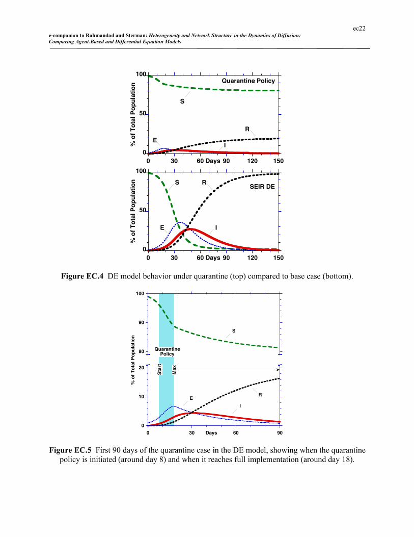
Figure EC.4 compares the results of the quarantine policy to the no-quarantine base case for
the DE model. Figure EC.5 shows the first 90 days in more detail, showing that contact reduc-
tion begins around day 8 and reaches full implementation around day 18. As expected, contact

ec21 e-companion to Rahmandad and Sterman: Heterogeneity and Network Structure in the Dynamics of Diffusion: Comparing Agent-Based and Differential Equation Models
reduction dramatically shortens the epidemic and reduces cumulative cases. In the base DE
model, F falls from 98% infected to 19%. The epidemic peaks after 31 days, compared to 48
days without quarantine, and with peak prevalence of infectious individuals of 4.4%, compared
to 27% in the base case. Due to the incubation time the peak of the infectious population lags
full implementation of contact reduction measures.
Note that the E and I populations decay quite slowly after full quarantine implementation.
The slow decay is due to the assumption that quarantine is imperfect. In the simulation R0 falls
to a minimum of about 0.6 at full implementation. Consequently some new cases continue to be
generated, lengthening the effective time constant for the decay of the infectious population.
Table 5 in the paper (repeated here as Table EC.6) compares Tp, Imax, and F in the AB models
to the base DE case. The base DE values of Tp and Imax fall within the interval capturing 95% of
the AB realizations in all network and heterogeneity conditions. The base DE value of F falls
inside the 95% confidence interval for all cases except the lattice.
The impact of the policy on the public health metrics is large compared to the variability in
the realizations of the individual AB simulations and in the variability of the metrics across net-
work and heterogeneity conditions.
Connected Random Scale-free Small World Lattice Metric H= H≠ H= H≠ H= H≠ H= H≠ H= H≠
µ 0.215 0.249 0.157 0.201 0.148 0.247 0.112 0.117 0.102* 0.099* Final Size F σ 0.084 0.091 0.064 0.088 0.062 0.105 0.044 0.048 0.037 0.035
µ 35.0 36.1 33.1 34.6 34.1 34.9 30.3 30.5 29.4 30.4 Peak Time Tp σ 15.3 15.9 14.8 16.7 15.7 18.1 13.5 14.2 13.5 14.6
µ 6.42 7.28 5.17 6.15 4.98 7.43 4.17 4.35 3.97 3.89 Peak Prev Imax σ 2.40 2.66 1.99 2.55 1.98 3.23 1.58 1.67 1.52 1.42
Table EC.6 Behavior of three public health metrics under the quarantine policy. */** indicates the value of the metric in the DE model falls outside the 95/99% confidence bound defined by the ensemble of AB simulations. The results for the DE model under quarantine are F = 0.190, Tp = 31.3 days, and Imax = 4.43%.
ec22 e-companion to Rahmandad and Sterman: Heterogeneity and Network Structure in the Dynamics of Diffusion: Comparing Agent-Based and Differential Equation Models
0
50
100
0 30 60 90 120 150
% o
f T
ota
l P
op
ula
tio
n
Days
S
EI
R
Quarantine Policy
0
50
100
0 30 60 90 120 150
% o
f T
ota
l P
op
ula
tio
n
Days
S
E I
RSEIR DE
Figure EC.4 DE model behavior under quarantine (top) compared to base case (bottom).
0
10
20
80
90
100
0 30 60 90
% o
f T
ota
l P
op
ula
tio
n
Days
E
I
R
QuarantinePolicy
Sta
rt
S
Max
Figure EC.5 First 90 days of the quarantine case in the DE model, showing when the quarantine policy is initiated (around day 8) and when it reaches full implementation (around day 18).

ec23 e-companion to Rahmandad and Sterman: Heterogeneity and Network Structure in the Dynamics of Diffusion: Comparing Agent-Based and Differential Equation Models
Another important question raised by the policy analysis is whether the differences between
the AB and DE models are large relative to the impact of the policy (the change in metrics from
the base case to the policy case). The change in a metric such as Tp or F is relevant because it
will inform the cost-benefit tradeoffs policymakers face. For example, policymakers may trade
off the cost of a policy against the number of cases avoided using some standard for the value of
a life, QALY or DALY. To address this question we need to find the change in each metric re-
sulting from the implementation of the policy across different AB scenarios and compare these
changes to the change in each metric for the DE case resulting from the implementation of the
same policy.
In each AB scenario we have 1000 simulations in the base case and 1000 in the policy case.
To assess the change in each metric as a result of policy implementation, we need to create a
one-to-one mapping between base case and policy simulations. However, there is no clear one-
to-one mapping between these simulations. For example, policy intervention in base simulation i
could have resulted in multiple policy simulation trajectories depending on the stochastic unfold-
ing of the policy case. Using the same random number seed in the base and policy simulations
of the AB model would not solve the problem because the sequence of particular contacts be-
tween infectious and susceptible individuals is endogenous and contingent on the impact of the
policy.
We estimate the change in each metric arising from the policy in the AB models as follows.
Each realization of the AB model in a given experimental condition in the base case (no policy)
is compared to a randomly selected realization of the AB model in that same condition in the
policy case. The change in the value of each metric ΔTp, ΔImax, and ΔF is calculated. This is re-
peated for each of the 1000 AB simulations in each experimental condition. Table EC.7 reports
the change in the metrics from the base case to the quarantine case using this procedure.

ec24 e-companion to Rahmandad and Sterman: Heterogeneity and Network Structure in the Dynamics of Diffusion: Comparing Agent-Based and Differential Equation Models
Connected Random Scale-free Small World Lattice Change in Metric
H= H≠ H= H≠ H= H≠ H= H≠ H= H≠
Mean 0.75 0.65 0.77 0.66 0.75 0.59 0.80 0.71 0.54 0.41 Change in Final Size ΔF = 0.793 σ 0.15 0.21 0.17 0.19 0.19 0.23 0.18 0.22 0.29 0.26
Mean 14.8 8.9 19.7 14.9 11.1 7.8 56.2 53.1 55.0 44.8 Change in Peak Time, ΔTp = 16.8 σ 18.8 20.7 20.1 22.2 20.2 22.5 34.7 39.6 59.1 52.4
Mean 22.6 19.9 21.3 18.9 21.8 17.9 14.0* 12.2* 5.3** 4.6** Change in Peak Prev, Δ Imax = 22.6 σ 5.5 6.8 5.5 6.2 6.3 7.3 5.2 5.6 3.7 3.7
Table EC.7 Change in metrics caused by the policy. The table shows the value of the metric in the base case less its value under the policy. */** indicates the change in the value of the metric in the DE model falls outside the 95/99% confidence bound defined by the ensemble of changes in pairs of AB simulations.
The difference between the base and policy values of Tp and F in the DE falls inside the 95%
interval of outcomes for all network and heterogeneity conditions. The difference between the
base and policy values of Imax in the DE falls within the 95% interval for all cases except the
small world and lattice. The policy impact is smaller in these conditions than in the DE because
the mean of Imax in the base-case AB model in these relatively clustered networks is smaller than
in the DE. In the base case heterogeneity generally lowers final size compared to the DE be-
cause highly connected individuals with high contact frequencies tend to become infected sooner
and are therefore removed from the infectious population sooner, lowering the mean contact fre-
quency for the remaining population. In contrast, under contact reduction, heterogeneity tends to
increase peak time. At the start of an outbreak the highly connected individuals fuel a quick
take-off, increasing the size of the exposed (asymptomatic) population before the first cases are
detected and the intervention can quench the epidemic. Consequently heterogeneity leads to
higher values of final size. As a result of these two effects, the mean values of ΔF in the hetero-
geneous cases of the AB model are smaller than the value generated by the DE. However, het-
erogeneity also increases outcome variability, so the range of outcomes caused by random inter-

ec25 e-companion to Rahmandad and Sterman: Heterogeneity and Network Structure in the Dynamics of Diffusion: Comparing Agent-Based and Differential Equation Models
actions among members of the population is larger, reducing the practical significance of the dif-
ferences in policy impact between the DE and AB models.
EC.10. Cost-Benefit Analysis and Policy Sensitivity
While the differences across network types and heterogeneity conditions is generally small
compared to the large impact of contact reduction, it is important to consider whether the differ-
ences in policy response might change the optimal policy set. Two models may have similar
overall base-case dynamics yet respond differently to policies. These differences might then
cause a different set of policies to be optimal. For simplicity, suppose that policymakers must
select either quarantine or no quarantine as discrete and mutually exclusive choices. Ignoring
uncertainty, quarantine will be optimal if its benefits B exceed its costs, C. The text provides an
example in which per capita quarantine costs are constant at C and the benefits are linear in
avoided cases, B = bΔF. The per capita benefits of each avoided case would include the value
assigned per life (or QALY or DALY), the monetary value of avoided health care costs and eco-
nomic losses arising from loss of tourism and business travel, disruptions to economic output and
supply chains, and so on.7 In this simple example, quarantine would be optimal if ΔF > C/b. As
shown in Table EC.7, the values of ΔF vary by network type and heterogeneity condition. For
example, in the scale-free case, ΔF is 0.75 for H= and 0.59 for H≠. Assuming there are no other
sources of uncertainty, the quarantine policy is optimal if C/b < 0.59 and no quarantine is opti-
mal if C/b > 0.75, independent of heterogeneity condition. However, for 0.59 ≤ C/b ≤ 0.75, the
optimal policy depends on whether the population is characterized by the H= or H≠ conditions:
in such a case the choice of model could have a large impact on policy.
Considering the range of outcomes across all network types and heterogeneity conditions
shown in Table EC.7, including the DE, quarantine is optimal if C/b < 0.41 and no-quarantine is
optimal if C/b > 0.80. Between these values the optimal policy depends on which network and
heterogeneity condition is judged most likely. To further complicate matters, the values of ΔF
7 In reality the economic costs of disruption and lost business are likely to be nonlinear: the small number of SARS cases in Toronto did not significantly depress travel and economic activity to the city, while the larger outbreaks in Hong Kong and Taiwan triggered large losses for the tourism and travel industries and substantial disruption to businesses. These social reactions are strongly conditioned by positive feedback processes including panic and bandwagon effects and are thus difficult to estimate.

ec26 e-companion to Rahmandad and Sterman: Heterogeneity and Network Structure in the Dynamics of Diffusion: Comparing Agent-Based and Differential Equation Models
used in these illustrative calculations are the means over the ensemble of 1000 AB realizations in
each condition. As seen in Table EC.7, there is substantial variability in the values of ΔF within
each condition. The mean of the standard deviations across all conditions is 0.21, so that the 2σ
range of variability in policy impact is roughly equal to the width of the region in which policy is
contingent on network type and heterogeneity condition (2σ = 0.42 ≈ 0.80-0.41). Further, the
values of ΔF will also vary over the range of uncertainty in parameters and model boundary.
Proper procedure would be for policymakers to construct the probability distribution characteriz-
ing the likelihood of each value of ΔF as it depends jointly on all sources of uncertainty, includ-
ing network topology, individual heterogeneity, parameters such as R0, the strength of social and
behavioral feedbacks, the costs of policy implementation and the benefits of avoided cases, then
select whether to implement the policy based on their tolerance for Type I and Type II error. In
practice, of course, such decision analysis is not done. Nevertheless, the results show that policy
choice can depend on the choice of model even when the base case behavior of the models is
similar. If policymakers judge that the parameters are such that the optimal policy is contingent
on model choice, then they should allocate additional resources to further empirical work de-
signed to resolve the uncertainty. To make that choice rationally requires that the value of in-
formation regarding all sources of model uncertainty be estimated through sensitivity analysis,
including analysis over network type, individual variability, model boundary, and so on. The
combinatorial explosion in the dimensionality of the required sensitivity analysis forces modelers
and policymakers to make tradeoffs imposed by limited time, budget, and computational re-
sources. Carrying out a full sensitivity analysis over policies, parameter uncertainty, network
and individual heterogeneity conditions, model boundary, and cost and benefits in an agent-
based model with realistic population size is infeasible. A more complete analysis can be carried
out in the computationally efficient DE, except that the DE, with its assumptions of homogene-
ous individuals and perfect within-compartment mixing cannot be used to test the impact of dif-
ferent network topologies and degrees of individual heterogeneity, unless it is disaggregated to
include additional compartments representing different types of individuals, locations in the con-
tact network, or other attributes.

ec27 e-companion to Rahmandad and Sterman: Heterogeneity and Network Structure in the Dynamics of Diffusion: Comparing Agent-Based and Differential Equation Models
Do calibrated DE models offer an efficient compromise? As shown in Tables EC.1 and
EC.2, the calibrated DE model fits individual realizations of the AB model well even though it
does not explicitly capture network clustering or individual heterogeneity. If the response of the
calibrated models to policy interventions is also similar to that of the AB models, then policy-
makers could use the computationally efficient calibrated DE models to explore policy impacts,
and, for any given budget and time frame, could carry out more sensitivity analysis than would
be possible in the computationally intensive AB model.
To test this hypothesis we conducted the following experiment. We simulated the contact re-
duction scenario in the DE model for every calibrated case (200 parameter sets in each of the ten
experimental conditions). In each, the contact rate was modeled using equations 6-7 in the paper.
The goal of this comparison is to determine whether the policy response of the calibrated DE
models is similar to the policy response of the AB models for the purpose of assessing the impact
of alternative policy interventions. Other purposes could also be considered, for example, fore-
casting the progression of an epidemic, designing studies to reduce uncertainty in key parameters
or test theories about modes of transmission, etc. Here we test whether the good fit of the cali-
brated DE models to the AB model outcomes implies that the policy response of the two model
types will be similar. Table EC.8 reports the results.
Connected Random Scale-free Small World Lattice Metric H= H≠ H= H≠ H= H≠ H= H≠ H= H≠
µ 0.212 0.105 0.111 0.075 0.112 0.061 0.135 0.083 0.064 0.047 Final Size F (0.190)
σ 0.122 0.041 0.040 0.030 0.044 0.026 0.054 0.034 0.040 0.025
µ 32.98 24.39 28.14 22.63 30.81 18.19 42.60 36.73 32.76 24.43 Peak Time Tp (31.3) σ
7.42 6.57 5.53 7.42 7.46 7.84 11.90 15.12 23.04 19.20 µ 4.35 3.41 3.27 2.74 3.02 2.61 2.65 2.19 1.75 1.72 Peak
Prev Imax (4.43)
σ 1.53 0.95 0.88 0.77 0.81 0.77 0.74 0.65 0.49 0.48
Table EC.8 Results of contact reduction in the calibrated DE models. Base DE values are re-ported in parentheses. The results should be compared with the Table EC.6, which reports the same metrics for the corresponding AB simulations. Mean values in italics show cases in which the calibrated DE provides a better fit to the AB means than the uncalibrated base case DE.

ec28 e-companion to Rahmandad and Sterman: Heterogeneity and Network Structure in the Dynamics of Diffusion: Comparing Agent-Based and Differential Equation Models
Comparing the results in tables EC.8 and EC.6 shows that, after application of the policy,
the DE models using the calibrated parameter values fail to show a high correspondence to the
corresponding AB simulations. The calibrated DE models provides a better fit to the mean of the
AB realizations for F and Tp in the homogeneous connected case, and Imax is nearly the same in
the calibrated and base cases. This is expected since the connected case is closest to the DE
model assumptions; differences among individual realizations reflect only the stochastic varia-
tion induced by random interpersonal contacts. In the heterogeneous connected case, however,
the uncalibrated base DE parameters provide a better fit to the mean of the AB realizations than
the calibrated models. Across the other conditions, the mean of the calibrated models provides a
better fit to the mean of the AB realizations only for F in the small world and lattice networks,
and in the H= scale free condition. The base model outperforms the mean of the calibrated mod-
els in all conditions for Tp and Imax (except as noted, for Tp in the H= connected case). The cali-
brated parameter values that successfully captured the network and heterogeneity effects in the
base case fail to capture those effects in the policy simulation.
The results show that the ability of the simple four-compartment deterministic SEIR model to
capture the base case behavior of individual AB epidemics does not imply that these simple
models can be used to assess the impact of policies. Further work is needed to explore the impli-
cations. Specifically, additional studies are required to determine the extent to which the results
arise from violations of the mixing and homogeneity assumptions vs. the stochastic variation in
individual realizations (Tables 3-4 and Figure EC.3 suggest both play a role). Additionally, fur-
ther work is required to determine whether disaggregating the DE models into more compart-
ments to capture key aspects of clustering and heterogeneity might improve the results, and how
AB simulation results might be used to find optimal partitions in such models.
EC.11. Simulating the model
Two versions of the model are posted with the online material. Both are developed in the
Anylogic ™ software. Anylogic supports both agent-based and differential equation models.
One interface is a stand-alone Java applet and runs under any Java-enabled browser with no need
to install additional software. The second includes the source code and equations of the model

ec29 e-companion to Rahmandad and Sterman: Heterogeneity and Network Structure in the Dynamics of Diffusion: Comparing Agent-Based and Differential Equation Models
and can be used for detailed inspection of model implementation and for simulation, once the
Anylogic software is installed.
To open the stand-alone applet, unzip “ABDE-Contagion-applet.zip” into one folder (all
three files need be in the same folder). You can then open the “Dynamics of Conta-
gion_Apr05_Paper Applet.html” file in any web browser (e.g. Internet Explorer). The interface
is self-explanatory and includes a help file, which can be opened by clicking the [?] button.
To open the Anylogic model source code, download and install the Anylogic software (a free
15-day trial is available at http://www.xjtek.com/download/). Unzip the attached file “ABDE-
Contagion-code.zip” in one folder. Open the file “Dynamics of Contagion_Apr05_Paper.alp” in
Anylogic. The list of all objects in the agent-based model is displayed in the left hand column;
select any object to inspect its formulation. Run the model by clicking on the run button (or
pressing F5), which compiles the model and brings up an interface similar to the Java applet.
You can inspect the behavior of the model both through the interface accompanying the model
and applet, or by browsing different variables and graphing them in Anylogic run mode. To do
the latter, go to “root” tab in run time mode, where you can see all model variables and can in-
spect their runtime behavior.
The implemented interface allows users to:
1. Run the model for different scenarios in single or multiple runs.
2. Inspect the behavior of the AB model, including the number of people in each state, state transition rates and user-specified confidence intervals for the infected population.
3. Visually inspect diffusion of the epidemic in the network. Different nodes and links between them are shown. You can choose among 4 different representations of the network structure to show the progression of the epidemic through the network.
4. Observe the metrics of peak value, peak time, and final size.
5. Change model parameters, including the incubation and recovery periods, infectivities, and contact rates (note that mean contact rates for exposed and infected individuals are expressed as fractions of the contact rate for healthy individuals). You can also set the size of the popu-lation, network type, number of links per person, and probability of long-range links in small-world network, and select the heterogeneous or homogeneous condition.
6. Save the results into a text file for subsequent analysis.

ec30 e-companion to Rahmandad and Sterman: Heterogeneity and Network Structure in the Dynamics of Diffusion: Comparing Agent-Based and Differential Equation Models
References
Anderson, R. M. and R. M. May 1991. Infectious diseases of humans dynamics and control. Ox-
ford University Press, Oxford.
Barabasi, A. L. and R. Albert. 1999. Emergence of scaling in random networks. Science 286
(5439) 509-512.
Fahse, L., C. Wissel and V. Grimm. 1998. Reconciling Classical and Individual-Based Ap-
proaches in Theoretical Population Ecology: A Protocol for Extracting Population Parame-
ters from Individual-Based Models. The American Naturalist 152(6) 838-852.
Newman, M. 2003. Random graphs as models of networks. Handbook of graphs and networks.
S. Bornholdt and H. G. Schuster, eds. Berlin, Wiley-VCH: 35-68.
Wallinga, J. and P. Teunis. 2004. Different epidemic curves for severe acute respiratory syn-
drome reveal similar impacts of control measures. American Journal of Epidemiology 160
(6) 509-516.
Watts, D. J. and S. H. Strogatz. 1998. Collective dynamics of "small-world" networks. Nature
393, 440-442.


