Center for UncertaintyQuantification
Center for UncertaintyQuantification
Center for Uncertainty Quantification Logo Lock-up
Hierarchical matrix approximation of
large covariance matricesA. Litvinenko1, M. Genton2, Ying Sun2, R. Tempone
1SRI-UQ Center and 2Spatio-Temporal Statistics & Data Analysis Groupat KAUST
Center for UncertaintyQuantification
Center for UncertaintyQuantification
Center for Uncertainty Quantification Logo Lock-up
Abstract
We approximate large non-structured covariance ma-trices in the H-matrix format with a log-linear com-putational cost and storage O(n log n). We computeinverse, Cholesky decomposition and determinant inH-format. As an example we consider the class ofMatern covariance functions, which are very popu-lar in spatial statistics, geostatistics, machine learningand image analysis. Applications are: kriging and op-timal design
1. Matern covariance
C(x, y) = C(|x−y|) = σ2 1
Γ(ν)2ν−1
(√2νr
L
)νKν
(√2νr
L
),
where Γ is the gamma function, Kν is the modifiedBessel function of the second kind, r = |x − y| andν, L are non-negative parameters of the covariance.
−2 −1.5 −1 −0.5 0 0.5 1 1.5 20
0.05
0.1
0.15
0.2
0.25
Matern covariance (nu=1)
σ=0.5, l=0.5
σ=0.5, l=0.3
σ=0.5, l=0.2
σ=0.5, l=0.1
−2 −1.5 −1 −0.5 0 0.5 1 1.5 20
0.05
0.1
0.15
0.2
0.25
nu=0.15
nu=0.3
nu=0.5
nu=1
nu=2
nu=30
As ν →∞ [4],
C(r) = σ2 exp(−r2/2L2).
When ν = 0.5, the Matern covariance is identical tothe exponential covariance function.
Cν=3/2(r) =
(1 +
√3r
L
)exp
(−√
3r
L
)
Cν=5/2(r) =
(1 +
√5r
L+
5r2
3L2
)exp
(−√
5r
L
).
Note: no need to assume neither C(x, y) = C(|x− y|) nor tensorgrid.
2. H-matrix approximation
25 20
20 20
20 16
20 16
20 20
16 16
20 16
16 16
19 20
20 19 32
19 19
16 16 32
19 20
20 19
19 16
19 16
32 32
20 20
20 20 32
32 32
20 19
19 19 32
20 19
16 16 32
32 20
32 32
20 32
32 32
32 20
32 32
20 19
19 19
20 16
19 16
32 32
20 32
32 32
32 32
20 32
32 32
20 32
20 20
20 20 32
32 32
32 32
32 32
32 32
32 32
32 32
32 32
20 2020 19
20 20 32
32 32 20
20 20
32 20
32 32 20
20 20
32 32
20 32 20
20 20
32 32
32 32 20
20
20 20
19 20 32
32 32
20 20
2032 20
32 32
20 20
2032 32
20 32
20 20
2032 32
32 32
20 20
20 20
20 20 32
32 32
20 19
20 19 32
32 32
20 20
19 19 32
32 32
20 20
20 20 32
32 32
32 20
32 32
32 20
32 32
32 20
32 32
32 20
32 32
32 32
20 32
32 32
20 32
32 32
20 32
32 32
20 32
32 32
32 32
32 32
32 32
32 32
32 32
32 32
32 32
20 20
20 20 2019 20
20 20 32
32 32
32 20
32 32
20 32
32 32
32 20
32 32
20 20
20 20
20 20
20 20 20
20 20
32 20
32 32 20
20 20
20 20
20 20
20 20 20
2032 20
32 32
20 20
20 20
20 20
20 20
20 20 2032 20
32 32
32 20
32 32
32 20
32 32
32 20
32 32
20 20
20 20
20 20
20 20
19 20
20 20 32
32 32
20 32
32 32
32 32
20 32
32 32
20 32
2020 20
20 20
20 20
20 20
20 20
32 32
20 32 20
2020 20
20 20
20 20
20 20
2032 32
20 32
20 20
2020 20
20 20
20 20
20 20
32 32
20 32
32 32
20 32
32 32
20 32
32 32
20 32
2020 20
20 20
20 20
20 20 32
32 32
32 32
32 32
32 32
32 32
32 32
32 32
19 19
20 20 32
32 32
32 20
32 32
20 32
32 32
32 20
32 32
19 20
19 20 32
32 32
20 32
32 32
32 32
20 32
32 32
20 32
20 20
20 20 32
32 32
32 32
32 32
32 32
32 32
32 32
32 32
20 20
32 32
32 32 20
20 20
32 20
32 32 20
20 20
32 32
20 32 20
20 20
32 32
32 32 20
2032 32
32 32
20 20
2032 20
32 32
20 20
2032 32
20 32
20 20
2032 32
32 32
20 20
32 32
32 32
32 32
32 32
32 32
32 32
32 32
32 32
32 20
32 32
32 20
32 20
32 20
32 32
32 20
32 20
32 32
20 32
32 32
20 32
32 32
20 20
32 32
20 20
32 32
32 32
32 32
32 32
32 32
32 32
32 32
32 32
25 9
9 20 9
920 7
7 169
9
20 9
9 20 9
9 329
9
20 9
9 20 9
9 32 9
932 9
9 32
9
9
20 9
9 20 9
9 32 9
9
20 9
9 20 9
9 329
9
32 9
9 32 9
932 9
9 32
9
9
20 9
9 20 9
9 32 9
932 9
9 329
9
20 9
9 20 9
9 32 9
932 9
9 32
9
9
32 9
9 32 9
932 9
9 329
9
32 9
9 32 9
932 9
9 32
Figure 2: Two approximation strategies [1]: fixed rank (left) andflexible rank (right) approximations, C ∈ Rn×n, n = 652.
I
I
I I
I
I
I I I I1
1
2
2
11 12 21 22
I11
I12
I21
I22
QQ t
S
dist
H=
t
s
1. Build cluster tree TI, I = {1, 2, ..., n}2. Build block cluster tree TI×I3. For each (t× s) ∈ TI×I, t, s ∈ TI, check admissibility
condition min{diam(Qt), diam(Qs)} ≤ η ·dist(Qt, Qs).
if(adm=true) then M |t×s is a rank-k matrix blockif(adm=false) then divide M |t×s further or define as adense matrix block, if small enough.
Grid → cluster tree (TI) + admissibility condition →block cluster tree (TI×I)→H-matrix→H-matrix arith-metics.
Operation Sequential Complexity Parallel Complexity(Hackbusch et al. ’99-’06) (Kriemann ’05)
storage(M) N = O(kn log n) NP
Mx N = O(kn log n) NP
M1 ⊕M2 N = O(k2n log n) NP
M1 �M2, M−1 N = O(k2n log2 n) NP +O(n)
H-LU N = O(k2n log2 n) NP +O(k
2n log2 nn1/d
)
Table 1: Computational cost of H-matrix arithmetics, sequentialand parallel.
Let ε =‖(C−CH)z‖2‖C‖2‖z‖2 , where z is a random vector.
n rank k size, MB t, sec. ε maxi=1..10
|λi − λi|, i ε2
for C C C C C4.0 · 103 10 48 3 0.8 0.08 7 · 10−3 7.0 · 10−2, 9 2.0 · 10−4
1.05 · 104 18 439 19 7.0 0.4 7 · 10−4 5.5 · 10−2, 2 1.0 · 10−4
2.1 · 104 25 2054 64 45.0 1.4 1 · 10−5 5.0 · 10−2, 9 4.4 · 10−6
Table 2: Accuracy of the H-matrix approx. exp. covariance function, l1 = l3 =0.1, l2 = 0.5.
l1 l2 ε
0.01 0.02 3 · 10−2
0.1 0.2 8 · 10−3
0.5 1 2.8 · 10−5
Table 3: Dependence of the H-matrix accuracy on the covari-ance lengths l1 and l2, n = 1292. The smaller cov. length the lessaccurate is H-approximation.
0
100
200
300
0
50
100
150
200
250
300
−1
0
1
2
−1
−0.5
0
0.5
1
1.5
2
2.5
3
0
100
200
300
0
50
100
150
200
250
300
−1
0
1
2
−3
−2
−1
0
1
2
Figure 4: Two realizations of random field generated viaCholesky decomposition of Matern covariance matrix, ν = 0.4.
3. Kullback-Leibler divergence
Measure of the information lost when distribution Q is used toapproximate P .
DKL(P‖Q) =∑i
P (i) lnP (i)
Q(i), DKL(P‖Q) =
∫ ∞−∞
p(x) lnp(x)
q(x)dx,
where p, q densities of P and Q. For miltivariate normal distribu-tions (µ0,C) and (µ1,C
H):
2DKL(N0‖N1) =
(tr((CH)−1C) + (µ1 − µ0)T (CH)−1(µ1 − µ0)− n− ln
(detC
detCH
)).
0 10 20 30 40 50 60 70 80 90 100−16
−14
−12
−10
−8
−6
−4
−2
0
rank k
log(r
el.
err
or)
Spectral norm, L=0.1, nu=0.5
Frob. norm, L=0.1
Spectral norm, L=0.2
Frob. norm, L=0.2
Spectral norm, L=0.5
Frob. norm, L=0.5
0 10 20 30 40 50 60 70 80 90 100−18
−16
−14
−12
−10
−8
−6
−4
−2
0
rank k
log(r
el.
err
or)
Spectral norm, L=0.1, ν=1.5
Frob. norm, L=0.1
Spectral norm, L=0.2
Frob. norm, L=0.2
Spectral norm, L=0.5
Frob. norm, L=0.5
Figure 5: RelativeH-matrix approx. error ‖C−CH‖2 for differentcov. lengths L = {0.1, 0.2, 0.5} and ν = {0.5, 1.5}
k KLD(C,CH) ‖C −CH‖2 ‖C(CH)−1 − I‖2L = 0.25 L = 0.75 L = 0.25 L = 0.75 L = 0.25 L = 0.75
5 0.51 2.3 4.0e-2 0.1 4.8 636 0.34 1.6 9.4e-3 0.02 3.4 228 5.3e-2 0.4 1.9e-3 0.003 1.2 810 2.6e-3 0.2 7.7e-4 7.0e-4 6.0e-2 3.112 5.0e-4 2e-2 9.7e-5 5.6e-5 1.6e-2 0.515 1.0e-5 9e-4 2.0e-5 1.1e-5 8.0e-4 0.0220 4.5e-7 4.8e-5 6.5e-7 2.8e-7 2.1e-5 1.2e-350 3.4e-13 5e-12 2.0e-13 2.4e-13 4e-11 2.7e-9
Table 4: Dependence of KLD on H-matrix rank k, Matern co-variance with L = {0.25, 0.75} and ν = 0.5, domain G = [0, 1]2,‖C(L=0.25,0.75)‖2 = {212, 568}.
For ν = 1.5 the KLD and the inverse (CH)−1 is hard to computenumerically. Results in Table 4 are better since covariance ma-trix with ν = 0.5 has smallest eigenvalues far enough from zero.The case ν = 1.5 is more smooth, the eigenvalues decay faster,but the smallest eigenvalues come much closer to zero than inν = 0.5 case.
4. Other applications
4.1 Low-rank approximation of Kriging and geo-statistical optimal designLet s ∈ Rn to be estimated, Css covariance matrix, y ∈ Rm isvector of measurements. The corresponding cross- and auto-covariance matrices are denoted by Csy and Cyy, respectively,sized n×m and m×m.
Kriging estimate s = CsyC−1yy y .
The estimation variance σ is the diagonal of the cond. cov. ma-trix Css|y: σs = diag(Css|y) = diag
(Css −CsyC
−1yyCys
)Geostatistical optimal design:
φA = n−1 trace[Css|y
]φC = cT
(Css −CsyC
−1yyCys
)c, c− a vector.
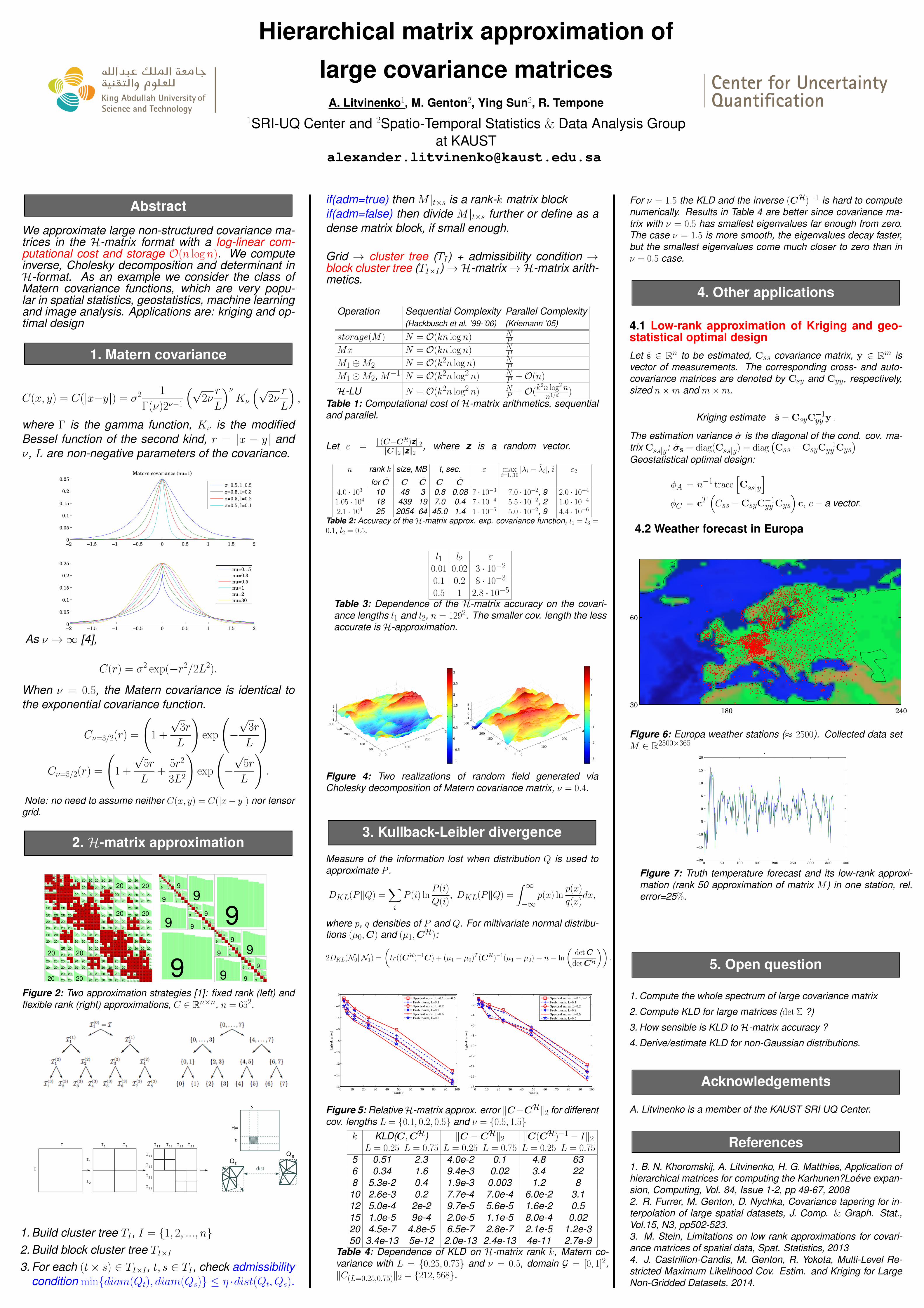
4.2 Weather forecast in Europa
180 24030
60
Figure 6: Europa weather stations (≈ 2500). Collected data setM ∈ R2500×365
.
0 50 100 150 200 250 300 350 400−20
−15
−10
−5
0
5
10
15
20
Figure 7: Truth temperature forecast and its low-rank approxi-mation (rank 50 approximation of matrix M ) in one station, rel.error=25%.
5. Open question
1. Compute the whole spectrum of large covariance matrix
2. Compute KLD for large matrices (det Σ ?)
3. How sensible is KLD to H-matrix accuracy ?
4. Derive/estimate KLD for non-Gaussian distributions.
Acknowledgements
A. Litvinenko is a member of the KAUST SRI UQ Center.
References
1. B. N. Khoromskij, A. Litvinenko, H. G. Matthies, Application ofhierarchical matrices for computing the Karhunen?Loeve expan-sion, Computing, Vol. 84, Issue 1-2, pp 49-67, 20082. R. Furrer, M. Genton, D. Nychka, Covariance tapering for in-terpolation of large spatial datasets, J. Comp. & Graph. Stat.,Vol.15, N3, pp502-523.3. M. Stein, Limitations on low rank approximations for covari-ance matrices of spatial data, Spat. Statistics, 20134. J. Castrillion-Candis, M. Genton, R. Yokota, Multi-Level Re-stricted Maximum Likelihood Cov. Estim. and Kriging for LargeNon-Gridded Datasets, 2014.


