
Project Number: GSF113
Hierarchical Swarm Robotics
A Major Qualifying Project Report
Submitted to the Faculty of the
WORCESTER POLYTECHNIC INSTITUTE
in partial fulfillment of the requirements for the
Degree of Bachelor of Science in Robotics Engineering
by
Nicholas Alunni Richard Goloski
Andrew Haggerty Eric Jones
X________________________ X________________________ X________________________ X________________________
Date: 4/28/2011
Approved:
______________________________ Prof. Gregory Fischer, Major Advisor
________________________________ Prof. Stephen S. Nestinger, Co-Advisor

Hierarchical Swarm Robotics i Worcester Polytechnic Institute 2011
Abstract Distributed computing is becoming more and more prevalent in engineering today. Swarm
robotics is simply an extension of that, not only dividing the computing power, but also the physical
capabilities. This project served as a proof of concept investigation into the feasibility and potential
effectiveness of a hierarchical swarm topology (HST), which better mimics the organization of many
societal structures. This goal was approached by designing a three-tier robotic swarm as well as a
specialized abstract coverage algorithm designed to map an unknown area. Experiments were
conducted by modifying the total number of robots in the HST. Results supported the original
hypothesis that by adding robots, overall runtime and individual workload is reduced.

Hierarchical Swarm Robotics ii Worcester Polytechnic Institute 2011
Table of Contents Abstract .......................................................................................................................................................... i
Table of Figures ............................................................................................................................................. v
Executive Summary ....................................................................................................................................... 1
Introduction .................................................................................................................................................. 2
Background ................................................................................................................................................... 5
Swarm Robotics ........................................................................................................................................ 5
Swarm Intelligence .................................................................................................................................... 6
Swarm Advantages.................................................................................................................................... 7
Swarm Disadvantages ............................................................................................................................... 9
Swarm Topologies ................................................................................................................................... 10
Coverage Algorithms ............................................................................................................................... 11
Previous Hierarchical Swarm Attempts .................................................................................................. 12
Hierarchal Swarm Topology ........................................................................................................................ 13
Structure ................................................................................................................................................. 14
Analogy of Structure ............................................................................................................................... 15
Delegation of Work and Information ...................................................................................................... 16
Pros and Cons of HST .............................................................................................................................. 17
Application Ideas ..................................................................................................................................... 17
Our Swarm .................................................................................................................................................. 18
Problem ................................................................................................................................................... 18
Breakdown of Hierarchy ......................................................................................................................... 18
Queen / Worker .................................................................................................................................. 19
Scout ................................................................................................................................................... 20
Budget ..................................................................................................................................................... 21
Methodology ........................................................................................................................................... 22
Mechanical .......................................................................................................................................... 22
Electrical .............................................................................................................................................. 22
Low-Level Software ............................................................................................................................. 23
High-Level Software ............................................................................................................................ 23
Mechanical Design .................................................................................................................................. 23
Material Choice ................................................................................................................................... 24
Hierarchical Swarm Robotics iii Worcester Polytechnic Institute 2011
Drivetrain Selection ............................................................................................................................. 25
Robot Design ....................................................................................................................................... 27
Electrical Design ...................................................................................................................................... 32
Queen and Worker.............................................................................................................................. 33
Design Requirements ...................................................................................................................... 33
MobileBoard ....................................................................................................................................... 33
Design Requirements ...................................................................................................................... 34
Power Supplies ................................................................................................................................ 34
Motor Control ................................................................................................................................. 35
Object and Heat Detection ............................................................................................................. 36
Localization Sensors ........................................................................................................................ 36
Wireless Communication ................................................................................................................ 37
Processor Selection ......................................................................................................................... 38
Circuit Design .................................................................................................................................. 39
Software Design ...................................................................................................................................... 41
Coverage Algorithm ............................................................................................................................ 42
Thinking in Bubbles ......................................................................................................................... 42
Description of Coverage Algorithm Basics ...................................................................................... 46
Greedy Algorithm Vs. Optimal Solution .......................................................................................... 47
Rules of the Coverage Algorithm .................................................................................................... 47
Heuristics of the Coverage Algorithm ............................................................................................. 50
In-depth Description of the Coverage Algorithm............................................................................ 53
Other Interesting Features .............................................................................................................. 57
Later Additions to the Algorithm .................................................................................................... 60
Mapping .............................................................................................................................................. 61
Data Representation ....................................................................................................................... 62
Interpreting Incoming Data ............................................................................................................. 65
Dijkstra’s Algorithm ............................................................................................................................. 67
Path Planning ...................................................................................................................................... 68
Communication ................................................................................................................................... 70
Scout Code .......................................................................................................................................... 72
Using μC/OS-II for this project ............................................................................................................ 74
Hierarchical Swarm Robotics iv Worcester Polytechnic Institute 2011
Board File ............................................................................................................................................ 76
Task organization ................................................................................................................................ 77
Experiments ................................................................................................................................................ 79
Simulation ............................................................................................................................................... 79
Data Collection ........................................................................................................................................ 81
Results ......................................................................................................................................................... 85
Mechanical Results ................................................................................................................................. 85
Electrical Results ..................................................................................................................................... 86
Software Results ..................................................................................................................................... 88
Discussion................................................................................................................................................ 92
Future Work ................................................................................................................................................ 93
Node Failure Detection ........................................................................................................................... 93
Emergency Stop / Other Safeties ............................................................................................................ 94
SLAM and the UKF................................................................................................................................... 95
Social Implications ................................................................................................................................ 100
Conclusion ................................................................................................................................................. 101
Bibliography .............................................................................................................................................. 102

Hierarchical Swarm Robotics v Worcester Polytechnic Institute 2011
Table of Figures
Figure 1: The structure before the addition of another mid level node (top), the structure after the
addition of another mid level node (bottom). Notice that the workload of all mid level nodes has been
reduced as a consequence. ........................................................................................................................... 4
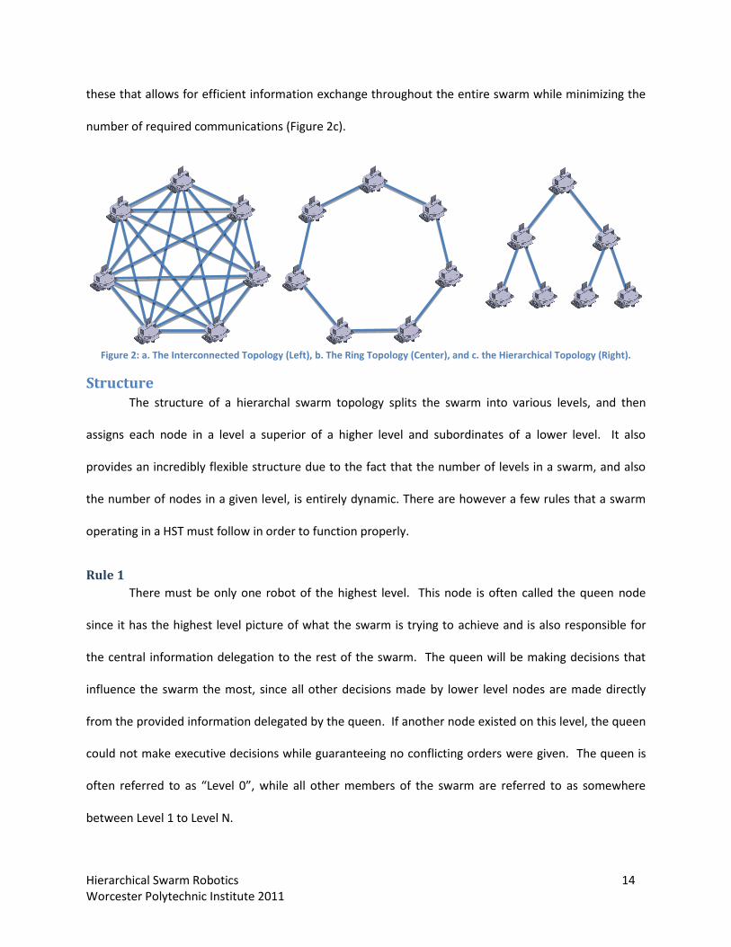
Figure 2: a. The Interconnected Topology (Left), b. The Ring Topology (Center), and c. the Hierarchical
Topology (Right). ......................................................................................................................................... 14
Figure 3: The three-level swarm to be implemented ................................................................................. 19
Figure 4: Gantt charts for the mechanical, electrical, and software design. .............................................. 23
Figure 5: Table comparing various materials for use on the robot. ........................................................... 25
Figure 6: A comparison of common drivetrains. ........................................................................................ 26
Figure 7: Initial CAD drawing of the robot. ................................................................................................. 28
Figure 8: First assembled prototype of the robot. ...................................................................................... 29
Figure 9: Second prototype of the robot - now with holders for the quadrature encoders. ..................... 30
Figure 10: Enclosure (sled) for a single mouse sensor. ............................................................................... 31
Figure 11: The final, fully assembled robot with encoders, wheels, PCB, and sensor turret. .................... 32
Figure 12: Comparison of the MSP430F5438 and the Xmega128A1. ......................................................... 39
Figure 13: Circuit of the N-Channel MOSFET and two pull up resistors. .................................................... 40
Figure 14: The finished board with all major components labeled. ........................................................... 41
Figure 15: Three different ways of gathering information in a bubble. Using a sharp IR sensor (left),
driving to all points in the bubble (center), and breaking the bubble up further for children (right). ....... 44
Figure 16: Diagram of the swarm and various bubbles used. Note that the queen is unable to see how
the workers are populating their bubble and different bubbles on the same level involve zero overlap. 45
Figure 17: A robot using a square bubble (Left). A robot using an amorphous bubble (Right). ................ 46
Figure 18: A sample of how the bubbles might be placed by the coverage algorithm. Note that none of
the bubble centers are in unknown space and none of the bubbles overlap. ........................................... 48

Hierarchical Swarm Robotics vi Worcester Polytechnic Institute 2011
Figure 19: Depiction of a level 2 robot (bubble shown in green) scanning within a level 1 robot’s bubble
(shown in blue). Since the level 2 robot’s bubble extends beyond the Level 1 robot’s bubble, none of the
information outside the level 1 robot’s bubble (shown as the grey squares) will be saved. ..................... 49
Figure 20: Valid placement of children by the coverage algorithm (left), invalid placement by the
coverage algorithm (right). ......................................................................................................................... 49
Figure 21: A nearly completed map with four robots attempting to scan. Three of the robots are capable
of scanning with their minimum radii; however a fourth robot cannot be placed without bubble overlap.
.................................................................................................................................................................... 51
Figure 22: Picture of various locations a robot could move to and scan with a radius of 3 cells and their
corresponding value. The location marked 35 is highest value because it scanning at that location would
uncover a high number of cells without much driving. The locations marked 25 and 15 are progressively
lesser value due to the fact that they uncover a similar number of cells however require significantly
more travel. The last location marked 2 is lowest value due to the fact that it is close, however scanning
there would not uncover a large number of cells....................................................................................... 52
Figure 23: Picture of robot scanning in known space, uncovering no new information (left). If the robot
is placed on the boarder of known and unknown space it is a guarantee that at least one new cell of
information will be uncovered (right). ........................................................................................................ 53
Figure 24: Pseudo code description of the coverage algorithm. ................................................................ 54
Figure 25: Picture of a map showing locations that are valid and drivable, as well as valid and un-
drivable. ...................................................................................................................................................... 56
Figure 26: Picture of the “closest robot” calculations. The robot in the center would be deemed the
closest since the sum of its distances to the other robots will be the minimum of the four robots shown
on the map. ................................................................................................................................................. 58
Figure 27: Picture of an idle robot moving out of the way so that it does not interfere with the scanning
robot. .......................................................................................................................................................... 60
Figure 28: A few sample Gaussian PDFs. This figure shows how the probability a given cell is blocked is
wider spread for higher standard deviations.............................................................................................. 63
Figure 29: Map offset example. The child working on the sub-problem defined by the blue bubble only
needs to store the blue square in memory. In order to ensure that coordinates are accessed globally,
the offset of (x’, y’) is needed so that (0, 0) will reference the same point for all robots. ......................... 65
Figure 30: Example of shadowing. Note that the blocked cell (colored black) causes all cells colored gray
to be shadowed. ......................................................................................................................................... 66

Hierarchical Swarm Robotics vii Worcester Polytechnic Institute 2011
Figure 31: Two examples of ray-tracing. ..................................................................................................... 66
Figure 32: Various stages of path optimization. ......................................................................................... 69
Figure 33: Three examples of conflicting paths requiring children to be sent in different waves. ............ 70
Figure 34: Sample code from the xmega128a1_board.c file. ..................................................................... 77
Figure 35: The simulation in progress of scanning a 5m x 2.5m map with two workers and four scouts. 81
Figure 36: Average scan are of the Level 1 and Level 2 robots compared to the total number of robots. 82
Figure 37: Average scan are of level 2 robots compared to the total number of robots. .......................... 83
Figure 38: Average drive distance of Level 2 and Level 1 robots compared to the total number of robots.
.................................................................................................................................................................... 84

Hierarchical Swarm Robotics 1 Worcester Polytechnic Institute 2011
Executive Summary This project aimed to be a proof of concept hierarchical swarm system. The idea for the project
resulted from observing the inefficiencies of traditional swarm communications which often utilize the
interconnected topology. A hierarchical swarm mimics the societal structure often used by humans by
using a tree-like communication topology. Specifically, the robots form a hierarchy which only allows a
robot to talk to its parent or its direct children. This also implies that no one robot is aware of the
number of levels in the swarm or the number of total robots involved. Due to the fact that any one
robot only is responsible for coordinating a small subset of the entire swarm, the computations and
communications required are reduced.
This project implemented a three level system with one robot on level 0, two robots on level 1,
and four robots on level 2 of the communication tree. The goal of the swarm was to autonomously map
an unknown area. The data collected from this swarm aims to prove the validity of the hierarchical
topology as well as show its future for expandability. Data was collected by creating virtual
representations of every robot in the swarm allowing for testing on swarms much larger than could
physically be built.
Autonomous mapping was performed by using an abstract coverage algorithm utilizing the
concept of a bubble. A bubble is an area in which a robot can gather information. Each robot in the
swarm can be abstracted to a bubble allowing any member of the swarm to map an area in a different
way. This can be used to take advantage of the hierarchical communications which allows a robot to
distribute tasks to children to increase parallelization.
Robots were constructed to show that a physical implementation of the swarm architecture was
possible. The robots were capable of traversing a flat terrain and mapping an area with IR rangefinders.

Hierarchical Swarm Robotics 2 Worcester Polytechnic Institute 2011
The robots were also capable of localization through odometry. Lastly, a custom PCB was designed to
allow for the use of all required sensors.
The project did successfully implement a three tiered swarm which was able to successfully map
an unknown area. The simulation was also effective at providing a means for further data collection
allowing meaningful data to be collected regarding the expandability of the swarm architecture. The
data collected shows that the amount of work for any member of the swarm is directly related to the
total number of robots in the swarm. The combination of a working physical swarm, a working and
expandable virtual simulation, as well as the data collected proves the viability of a hierarchical swarm
system. This project serves as an introduction into the hierarchical concepts with hope that further
research would follow.
Introduction Swarm robotics aims to solve complex problems using multi-agent systems, often mimicking real
life entities. The very name “swarm” comes from watching already existing collections of animals, such
as insects, packs, or flocks, and attempting to implement the observed behaviors in an unknown
environment. Swarm robotics, while broad, has a few defining characteristics. It deals exclusively with a
multi-nodal system, often working on problems where a distributed approach to the solution will serve
better than centralized control.
Swarm Intelligence encompasses the set of patterns which emerge from a set of robots
interacting with each other. The swarm is sometimes modeled after an already existing animal
population. There are a variety of popular swarm models, each aimed at solving a different type of task.
There is the Ant Algorithm, which attempts to mimic the pheromone tracking performed by ants when
moving to and from a food source [1]. Another algorithm that related to finding food is the Bee
Algorithm, which mimics the behavior of bees when searching for nectar [2]. A more general algorithm

Hierarchical Swarm Robotics 3 Worcester Polytechnic Institute 2011
aimed at finding resources in an unknown location is known as the PSO or Particle Swarm Optimization
algorithm which is designed to best approximate flocks of birds looking for a single meal in a large,
unknown area [3]. While the application of all swarms remains relatively vast, one commonplace factor
is the simplicity of the algorithms. They are often built with a very small number of behaviors,
sometimes as few as one concrete rule.
Another issue that often appears in the set of problems well suited to a multi-agent system is
the concept of area coverage where a set of mobile-nodes are attempting to fully uncover an either
known or unknown area [4]. The basis for the field is laid in investigating how a single robot would span
a given space, and is then adapted to the multiple robot system [5] [6]. While coverage algorithms are
not the main focus of this project, they were a substantial portion of the implementation.
However, what appears to be an often overlooked concept when it comes to the optimization of
any such algorithms is the topology, or interconnectivity of the various nodes of a swarm. The two most
common topologies of a distributed agent system are the interconnected and ring topologies [7] [8] [9].
An interconnected topology works by allowing every node to communicate with every other node in the
swarm. Ring topology allows a node to communicate with two adjacent nodes. Other implementations
have at times been suggested but appear to be studied in relatively limited amounts. This project aims
to expose the feasibility and future optimization of a new topology; a hierarchical structure modeled
closely to the natural simplification of information handling and distribution in today’s society.
The first rule when forming a Hierarchical Swarm Topology (HST) is that any node may only talk
to its direct superior or its subordinate(s). The HST also stipulates that unlike a traditional single level
swarm which uses the fully connected or ring topology; nodes cannot communicate with nodes on their
own level. This structure allows for a robust template to be used when passing out information and
responsibilities.

Hierarchical Swarm Robotics 4 Worcester Polytechnic Institute 2011
While we aim to implement a coverage algorithm using a HST, the other goal of this project is to
demonstrate the highly scalable swarm communication architecture resulting from the rules of the HST.
The main advantage of an HST comes from its significantly reduced number of communications when
compared to a variety of other topologies. The second advantage comes from the scalable nature of the
HST. If a communication bottleneck is reached at any point between a superior and its subordinates, a
new superior (of the same level as the original) can be created and assigned a portion of the original
superior’s subordinates, thereby easing the load on all parties.
Figure 1: The structure before the addition of another mid level node (top), the structure after the addition of another mid level node (bottom). Notice that the workload of all mid level nodes has been reduced as a consequence.
This project aims to set the foundation of future work in hierarchal swarm topologies. It will do
so by implementing the HST on a given problem - mapping an unknown area while looking for a certain
object. The goal is to also lay the basis for future work to be done using the HST. Specifically, the swarm
Hierarchical Swarm Robotics 5 Worcester Polytechnic Institute 2011
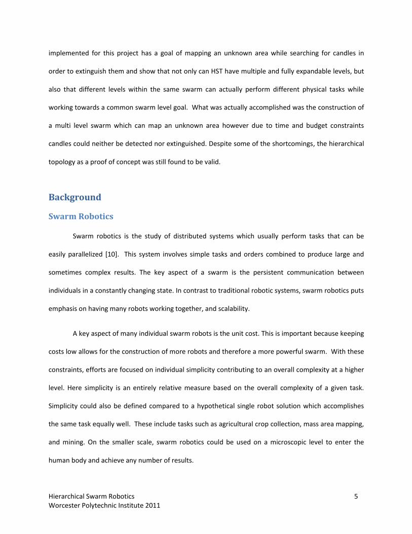
implemented for this project has a goal of mapping an unknown area while searching for candles in
order to extinguish them and show that not only can HST have multiple and fully expandable levels, but
also that different levels within the same swarm can actually perform different physical tasks while
working towards a common swarm level goal. What was actually accomplished was the construction of
a multi level swarm which can map an unknown area however due to time and budget constraints
candles could neither be detected nor extinguished. Despite some of the shortcomings, the hierarchical
topology as a proof of concept was still found to be valid.
Background
Swarm Robotics
Swarm robotics is the study of distributed systems which usually perform tasks that can be
easily parallelized [10]. This system involves simple tasks and orders combined to produce large and
sometimes complex results. The key aspect of a swarm is the persistent communication between
individuals in a constantly changing state. In contrast to traditional robotic systems, swarm robotics puts
emphasis on having many robots working together, and scalability.
A key aspect of many individual swarm robots is the unit cost. This is important because keeping
costs low allows for the construction of more robots and therefore a more powerful swarm. With these
constraints, efforts are focused on individual simplicity contributing to an overall complexity at a higher
level. Here simplicity is an entirely relative measure based on the overall complexity of a given task.
Simplicity could also be defined compared to a hypothetical single robot solution which accomplishes
the same task equally well. These include tasks such as agricultural crop collection, mass area mapping,
and mining. On the smaller scale, swarm robotics could be used on a microscopic level to enter the
human body and achieve any number of results.
Hierarchical Swarm Robotics 6 Worcester Polytechnic Institute 2011
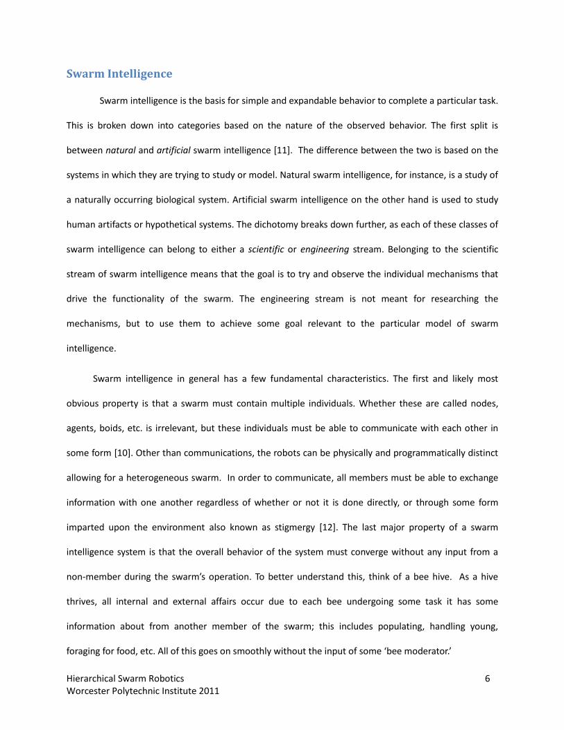
Swarm Intelligence
Swarm intelligence is the basis for simple and expandable behavior to complete a particular task.
This is broken down into categories based on the nature of the observed behavior. The first split is
between natural and artificial swarm intelligence [11]. The difference between the two is based on the
systems in which they are trying to study or model. Natural swarm intelligence, for instance, is a study of
a naturally occurring biological system. Artificial swarm intelligence on the other hand is used to study
human artifacts or hypothetical systems. The dichotomy breaks down further, as each of these classes of
swarm intelligence can belong to either a scientific or engineering stream. Belonging to the scientific
stream of swarm intelligence means that the goal is to try and observe the individual mechanisms that
drive the functionality of the swarm. The engineering stream is not meant for researching the
mechanisms, but to use them to achieve some goal relevant to the particular model of swarm
intelligence.
Swarm intelligence in general has a few fundamental characteristics. The first and likely most
obvious property is that a swarm must contain multiple individuals. Whether these are called nodes,
agents, boids, etc. is irrelevant, but these individuals must be able to communicate with each other in
some form [10]. Other than communications, the robots can be physically and programmatically distinct
allowing for a heterogeneous swarm. In order to communicate, all members must be able to exchange
information with one another regardless of whether or not it is done directly, or through some form
imparted upon the environment also known as stigmergy [12]. The last major property of a swarm
intelligence system is that the overall behavior of the system must converge without any input from a
non-member during the swarm’s operation. To better understand this, think of a bee hive. As a hive
thrives, all internal and external affairs occur due to each bee undergoing some task it has some
information about from another member of the swarm; this includes populating, handling young,
foraging for food, etc. All of this goes on smoothly without the input of some ‘bee moderator.’

Hierarchical Swarm Robotics 7 Worcester Polytechnic Institute 2011
Swarm Advantages
The advantages and disadvantages of using a robotic swarm versus a conventional single-robot
solution are heavily dependent on the problem being approached. A common advantage of using a
robotic swarm is when the fundamental problem to be solved is coverage. For instance, in military
operations using a robotic swarm to defuse a bomb does not take advantage of anything it has to offer
because the task cannot easily be parallelized. On the other hand, using a swarm of Unmanned Aerial
Vehicles (UAVs) for large scale surveillance is highly advantageous compared to trying to get the same
coverage using a single robot. Trying to survey the same effective area as a small swarm would be very
difficult and costly for a single robot. To be able to match the area and speed at which a number of
cheaper and simpler robots could do the task would require drastic increases in the quality and range of
the mobility and sensor systems onboard, and may still be inadequate in comparison.
Along with the idea of coverage, is the great potential for expandability. Single robot applications
have to be designed with tight task specifications in mind such as completion time. Proper engineering
will yield something capable of doing the designated goal sufficiently. If any goal becomes more difficult
to meet, (for instance, if the previously mentioned completion time is now shorter) there is a good
chance that it will require a lengthy and costly redesign. If a swarm is being designed, it is possible that
some of the requirements becoming tighter can be resolved by adding additional robots. There will be a
limit to this in most systems, but the ability to add more of the same hardware into the field should
increase the longevity of the design until the problem changes or grows far beyond the useful capacity of
a single swarm. Increasing the size of the swarm can also be used to enhance the number of redundant
systems to allow for fault-tolerance.
Implementing a swarm provides the possibility to make swarm members simpler. To offset the
limitations of each individual robot, there is the notion of parallel processing. This method utilizes the
fact that the swarm consists of many members to complete a task. For instance, if a large amount of

Hierarchical Swarm Robotics 8 Worcester Polytechnic Institute 2011
work needs to be done, it could be intelligently divided amongst the members to find multiple parts of
the solution simultaneously. This reduces the negative impact of using cheaper, less powerful hardware.
Along those same lines, simple physical tasks can also be accomplished in parallel rather than in series. If
a portion of the physical task can be assigned to each member of the swarm, it can be completed faster
than a single robot. As the task becomes more demanding, more members of the swarm can be added
while this would simply take more time for a single robot without a redesign.
By keeping item costs down and unit design simple, replacement and repair of these units is very
feasible. Since each unit only has a comparatively small investment behind its construction, they can be
used more liberally, particularly in potentially hazardous environments. The consequences of losing an
individual swarm member are much lower than losing the single robot. In a swarm with different types
of robots, tactical decisions could be made in dangerous situations to sacrifice the less valuable
members if necessary. As an extension of that, loss of a single swarm member does not mean the loss of
all of the information the group can gather; it simply weakens the swarm’s ability to gather information
and complete tasks relative to how many members remain and are necessary. Robots can be cycled out
of duty briefly while the remainder of the swarm continues to operate in case one is damaged or in need
of refueling. In a single-robot application, operations would have to cease during repairs or refueling.
In summation, the pros are:
More flexible coverage
Expandability
Fault-tolerance / Redundant systems
Parallelization
Reduced relative unit cost

Hierarchical Swarm Robotics 9 Worcester Polytechnic Institute 2011
Swarm Disadvantages
While swarm systems have many potential advantages over single agent systems, there are also
some downsides. Since a swarm depends on communication to function, bandwidth issues and
communication delays from long transmission paths can arise. Also, the simplistic nature of a robotic
swarm requires a cleverly designed system and impressive intelligence to be able to achieve physical
tasks that a single, larger unit can.
One of the major limitations in swarm robotics is the ceiling on communications. This ceiling
covers anything which will cause a bottleneck due to the finite speed at which data can be transferred.
For a reasonable number of robots sending non-trivial amounts of data, expanding a swarm quickly
becomes problematic in most topologies which negatively impacts scalability. Whether due to the
number of ‘hops’ made in order for data to reach its destination, the total number of communication
lines, or sheer transfer volume, there is a limit to any communication system. Different topologies
address different weaknesses in communication; however this will be discussed later. Similarly, individual
robots in a swarm may fall short of computing requirements due to their much simpler design. This
should ideally be avoided with proper allotment of labor, but it is an easy trap to fall into, as even the
most accurate CPU load prediction is not particularly useful if the software design has major changes.
Another potential disadvantage for a swarm is for accomplishing physical tasks (actuation and
mobility). Designing a single robot to physically accomplish a task is by no means trivial in most cases,
but is at least reasonably straightforward. To have a robotic swarm be able to achieve a similar task and
attempt to meet requirements will require very intuitive design, as well as very robust problem-solving.
For example, if the task is to drive a 1 pound payload across a 6 inch gap, it is simpler to have a single
robot carry the load across rather than have a swarm of robots where each share a part of the load.
In summation, here are the cons of using swarm robotics:
Hierarchical Swarm Robotics 10 Worcester Polytechnic Institute 2011
Communication bottlenecks
System design is more complex
Poor performance if task is not parallelizable
Swarm Topologies
While swarm robotics is still a fairly fresh concept, it still has some well-established topologies, as
well as some lesser-known, and more experimental ones [7]. Topologies exist to determine all channels
for communication between all agents in the swarm. Probably the simplest to understand is the
interconnected (or fully-connected) topology. In this configuration, every agent in the swarm
communicates with every other member. While this makes communicating between any two robots
trivial, this topology is not very expandable. For a swarm with n robots, each robot has to be able to
handle n – 1 communications at any time. This very swiftly creates a bottleneck even using a
communication method with high data-rates.
A common alternative to an interconnected topology is the ring topology [9]. Ring dictates that
each node is able to communicate with two neighbors. Through this requirement, the topology forms a
ring when all nodes are connected. Unlike an interconnected topology, ring doesn’t arrive at a
bandwidth bottleneck with swarm expansion, however the complexity required for decision-making and
the actual delay of communication from opposing sides of the ring can become a hindrance.
Another option is the “small-world” topology. This example may be a bit newer as a topology
compared to ring and interconnected, but has clearly begun proving its value (especially in PSO) [13].
The small-world topology goes off of the ideas of the “six degrees of separation”, such that each agent is
a small number of communication steps to reach any other agent. This greatly reduces the setbacks that
a ring topology encounters. As an extension of that, it also has less of a bandwidth bottleneck than
Hierarchical Swarm Robotics 11 Worcester Polytechnic Institute 2011
interconnected. While small-world has advantages over both ring and interconnected, it also has
weaknesses compared to each as well, but achieves a decent balance for greater expandability.
Coverage Algorithms
While topologies are very core to the implementation of a swarm system, the desired goal of this
project was mapping, which entails the use of a coverage algorithm. The concept of a coverage algorithm
is far from new in the realm of computer science. The goal of gathering complete information in an
unknown space has been researched before. The problem is not unique to robotic swarms or even
robots at all. As a general rule, coverage algorithms must be complete, but beyond this, the field
branches significantly. A few simple examples of single-agent coverage algorithms are the Backtracking
Spiral Algorithm (BSA) [5] and the Coverage Path Planning Algorithm (CPPA) [14]. In the former, the agent
undergoes a simple wall-following behavior, marking any scanned area as currently inaccessible. This will
eventually spiral inwards until all three sides are either blocked by an obstacle or marked as inaccessible.
At this point, the algorithm seeks the nearest point that hasn’t been scanned and starts a new spiral. The
latter, CPPA, is a bit more complicated, and has many variations. One case uses triangle meshing to
determine agent locations and a circle overlay to represent the robot’s useful area (whether it is
information gathering or physical size). When the circles cover the entire world, then it is complete, and
a path can be derived from the circumcenters of the triangles. Minimizing this path length optimizes this
version of the CPPA.
In order to determine what ‘coverage’ specifically means in the algorithm depends on the
desired task. For a mapping robot, full coverage is achieved when all sensor data used can construct a
complete picture of the map. This differs from a Roomba, which would achieve coverage by physically
driving through as much of the map as possible. Driving through the entire space is usually sufficient, but
not always necessary for all system models. In a scenario that simply requires data collection for finding

Hierarchical Swarm Robotics 12 Worcester Polytechnic Institute 2011
objects, driving through the space is not required as long as the robot has some kind of range-finding
sensor.
For systems with multiple agents (robots), many of the more rudimentary coverage approaches
fail, and some cannot even be easily adapted to the task. BSA for instance, does not lend itself well to
multiple-robot configurations, but some versions of CPPA can be fairly reasonably extended in order to
distribute work. The arc-coverage CPPA for instance, which uses laterally overlaid rounded rectangles for
maximum performance, must have a large adaptation to guarantee robots do not collide while covering
different areas due to intersecting paths[14]. The triangle meshing CPPA on the other hand generates a
single set of path points which can be split among robots, but does not take into account maps with
unreachable areas and assumes the space is fully accessible [15]. An example of an implemented multi-
robot application exists for boundary inspection [6]. This instance approached the problem using the k-
Rural Postman Problem (kRPP). While this case behaves fairly optimally, a truly optimal system using this
approach is NP-hard, so a heuristic was used instead.
Previous Hierarchical Swarm Attempts
The concept of a hierarchical topology in network systems has been recognized for its flexibility
and reasonable number of connections. The concept of a tree topology, (as it is also known in network
systems) is to have a single root node with at least two tiers of children below that (only one tier would
make it a star topology). Each tier lacks connections to nodes on the same tier, and only shares a
connection with one node at a depth one less than the current. That is to say, each node (except the
root) has one parent, and can have any number of children below it, including zero. This is a fairly useful
and simple system, often used in data structures as well for its efficiency.
As a topology for a robotic system, very little work has been done on the subject, but there is
one specific publication relevant enough to this paper to mention here. This research article discusses

Hierarchical Swarm Robotics 13 Worcester Polytechnic Institute 2011
the idea of allowing groups of robots nearby to form agents which self-organize to form collective
agents [8]. Each of these collective agents works as a group, with a single line of communication to other
agents; the hierarchy assembles as the groups contain groups, eventually consisting of the entire swarm.
Within each collective group, agents can be allowed to talk to one another, or potentially reorganize as
necessary. This ability to talk to one another on the same level is the main difference between the
research performed in that article and this project.
The publication goes on to test four variations on a three-tier hierarchical topology, the top level
and mid-level both being attempted with either interconnected or ring topologies. This was tested using
a variation of particle swarm optimization (PSO) known as PS2O, which implements PSO per level of the
swarm. In testing, the four variations of PS2O (for each ring/interconnected per level) outperformed
every other algorithm in the test for unimodal, multimodal, and discrete functions. In the benchmark
tests, the PS2Os performed the best in terms of convergence rate, accuracy, and robustness, not to
mention being the only ones to consistently complete and minimize a few of the tests.
Hierarchal Swarm Topology A hierarchal swarm topology works off the idea of having multiple levels within one operating
swarm. Traditionally most swarms work in a “flat” nature where although all the nodes may or may not
talk to each other, they are all considered as being on the same level. As stated earlier, traditional
swarms are implemented with either an interconnected topology (Figure 2a) or a ring topology (Figure
2b). The interconnected topology achieves the goal faster, but requires a significantly larger amount of
communication overhead and connection handling between each robot. The ring topology minimizes
the number of communications per robot, but causes information to be disseminated out to each node
significantly slower. The hierarchal swarm topology aims at a mixture of the function between both of
Hierarchical Swarm Robotics 14 Worcester Polytechnic Institute 2011
these that allows for efficient information exchange throughout the entire swarm while minimizing the
number of required communications (Figure 2c).
Figure 2: a. The Interconnected Topology (Left), b. The Ring Topology (Center), and c. the Hierarchical Topology (Right).
Structure The structure of a hierarchal swarm topology splits the swarm into various levels, and then
assigns each node in a level a superior of a higher level and subordinates of a lower level. It also
provides an incredibly flexible structure due to the fact that the number of levels in a swarm, and also
the number of nodes in a given level, is entirely dynamic. There are however a few rules that a swarm
operating in a HST must follow in order to function properly.
Rule 1
There must be only one robot of the highest level. This node is often called the queen node
since it has the highest level picture of what the swarm is trying to achieve and is also responsible for
the central information delegation to the rest of the swarm. The queen will be making decisions that
influence the swarm the most, since all other decisions made by lower level nodes are made directly
from the provided information delegated by the queen. If another node existed on this level, the queen
could not make executive decisions while guaranteeing no conflicting orders were given. The queen is
often referred to as “Level 0”, while all other members of the swarm are referred to as somewhere
between Level 1 to Level N.
Hierarchical Swarm Robotics 15 Worcester Polytechnic Institute 2011
Rule 2
Any node in the swarm can only communicate with its one superior node, and any of its own
subordinate nodes. The reason for this is to provide better structured communications. While a ring
topology also reduces communications compared with an interconnected topology, a ring topology
assumes that the neighboring nodes are the nodes most important to communicate with. The
hierarchical swarm topology allows for a better heuristic for selecting nodes to talk to. Communication
lines in a hierarchical structure are known to pass data relevant to both the sender and recipient.
Another important consequence of this is that any node in the swarm is strictly prohibited from
communicating with any other node of the same level.
Analogy of Structure The concept and implementation of an HST can be considered very similar to a police station. In
a police station there is often one chief. From there, there are many levels between the chief and the
lowest ranking officers. General directions and all the information is reported to the chief, who then
delegates out specific tasks to his/her subordinates. Each subordinate then uses the information they
have at hand to further delegate out the work and determine the best way to obtain more information
or perform a task. This process continues until you have the lowest level of police, which may be an
officer on patrol. Now, the reason this structure works is because while the police chief has the most
information, he/she does not have the time to actually do all of the police work him/herself. Just like in
an HST each level accomplishes their given task independent of their peers and report back to their
superior. The police chief would not have time to patrol every street on his/her own and nothing would
ever be done if every officer communicated amongst themselves to divide the workload.
Also very similar to a HST, is the dynamic nature of the police structure. For example if you look
at one particular part of the analogy, say the dispatcher taking in calls from the public and then giving
each call to a particular officer on the street to investigate, there is a limited number of officers that

Hierarchical Swarm Robotics 16 Worcester Polytechnic Institute 2011
each dispatcher can coordinate. However, if the police department continues to add officers to the
street, each one must also be assigned to a dispatcher until eventually that dispatcher becomes
overloaded. At that point, it becomes necessary to add another dispatcher into the police department
and give some of the work (officers) from the first dispatcher to the newly added one. That dispatcher
then also needs to be given a superior to report to. However, the rest of the department doesn’t have
to adapt to having a new dispatcher, no protocols need to be changed. The dispatcher’s superior simply
now has one more person to which work can be delegated (Figure 1).
The second rule from the structure is also well demonstrated in this analogy, given the fact that
two people of the same level should never be required to communicate. For example continuing with
the analogy from above there shouldn’t be a reason that two officers have to ask each other what to do,
they should always be going through their dispatcher when they need new information or work to be
assigned. Also each dispatcher has a different set of officers, so the information that either dispatcher
has is unlikely to be relevant to one another; therefore they should always go through their superior in
order to obtain instructions.
Delegation of Work and Information This section will mainly discuss how different types of problems could be solved with an HST and
the guidelines of how work should be delegated among the swarm. The goal is simply to convey the
basis for how problems should be solved, not actually give implementation notes. The reasons for this is
while the concepts should remain relatively universal, the actual implementation will and should change
depending on the particular problem trying to be solved.
In general, the solution of decision making of the swarm should be written in such a way that it
can be generalized to a multi-level system and so that the information gathered by the subordinates can
in some way be turned into the information needed by the higher levels. For example in PSO which

Hierarchical Swarm Robotics 17 Worcester Polytechnic Institute 2011
aims to find a “food source” with a large number of nodes, each node has to report back how close it is
to the given food source. With the HST, each of the subordinates would find their distance to the goal
and give that information to the superiors, who could then pass the group minimum up to the queen.
The important aspect is that the solutions should be designed in such a way that information can be
compiled into a form that can be sent up or down as many levels as needed without losing integrity.
Pros and Cons of HST One of the largest pros of hierarchical swarm systems is their scalability. Within this, there are
many smaller, yet important advantages. In swarm robotics, communication is always a very important
issue. There are many robots cross communicating constantly, with potentially high amounts of data. It is
necessary to be able to transmit and receive all this data without information being lost or dropped.
With hierarchical swarm systems, robots only communicate with their parents, and however many
children they have directly underneath them. This makes for much less overall communication to
perform the same amount of work. A robot “knows” any commands or data it receives can only come
from its parent or its children respectively. This directly influences scalability, because generally swarms
are limited by the amount of communication that can be handled. With less overall communication, the
scale of the swarm can be much larger.
Increasing the physical size of a hierarchical swarm is much easier than adding a robot in a
normal swarm system. In a non-hierarchical swarm, every robot has to be made aware that there is a
new robot in the swarm. In a hierarchical swarm, the new robot's parent and children are the only
robots that need to know about the addition. Also, more layers can be implemented as new robots are
added, keeping communications much simpler than regular swarm systems.
Application Ideas Hierarchical swarm systems can be applied to many different problems and situations. Area
mapping is one great use. The highest level can know the size of the area needed to be mapped and can

Hierarchical Swarm Robotics 18 Worcester Polytechnic Institute 2011
designate sections to lower levels, which can then be redistributed until the area is mapped and sent
back up the chain to the queen. A hierarchical swarm works particularly well for this application because
mapping is usually highly parallelizable and the hierarchical topology provides a mechanism for properly
distributing the workload. Also, different branches can be given different values based on their mapping
effectiveness and can be given areas to map that fit their value. Depending on the swarm and type of
robots, areas can be mapped that are as small as individual rooms or as large as full towns.
Our Swarm The following sections outline in detail the implementation of an HST for this particular project.
They discuss the structure of the HST, and then transition into the Mechanical, Electrical, and Software
components of the project.
Problem For this project the goal was to create a hierarchical swarm topology and use it to find and
extinguish simulated fires in an unknown space. In order to locate the fires the group needed to
implement a coverage algorithm that would ensure that the space was fully covered. The task was to be
implemented with a three level HST with one level 0, two level 1 robots and four level 2 robots. This
project also aimed to show the scalability of an HST by simulating the running of the swarm with more
robots than could be physically built. Although the firefighting goal was not completely met, many
design decisions were made in mind with allowing the goals to be completed eventually given enough
time or budget.
Breakdown of Hierarchy This section describes the capabilities and responsibilities of each level in the swarm. The
swarm consists of three levels, two of which are administrative and one of which is object detection.
While they share some code and abilities, the two administrative levels are significantly more complex.

Hierarchical Swarm Robotics 19 Worcester Polytechnic Institute 2011
The top level of the swarm is known as the queen or level 0 and controls the function and direction of
the entire swarm, specifically the second level. The second level is known as “the worker” or level 1 and
is directly under the control of the queen. The name is derived from the fact that it was originally
intended to be the level of the swarm responsible for extinguishing the fire. It will have the same basic
functionality as the queen however it only needs to be aware of a smaller sub section of the map. The
lowest level of the swarm being created known as “the scout” or Level 2 will be the physical interface of
the swarm and the outside world. While both levels 1 and 2 were intended to be mobile, level 2 is the
only level with actual sensors for scanning the world around it. An in-depth description of the various
levels of the swarm is below.
Figure 3: The three-level swarm to be implemented
Queen / Worker
The worker and queen both serve as directors of the swarm. The only difference between the
functionality of the two is that the queen will be able to see the entire map and the worker will utilize
sub-portions of the map assigned to it by the queen. However their operations on the map remain
identical. It was intentional that the queen and workers would divide the map in the same manner to be
Level 0 - Queen
Level 1 - Worker
Level 2 - Scout
Hierarchical Swarm Robotics 20 Worcester Polytechnic Institute 2011
completed by their children. In that way, it can be proven that the swarm could be expanded to an
arbitrary number of levels. The only changes needed would be to add more robots and assign the
correct parent-child relationships.
When either level 0 or 1 is told to map an area, both will run the same coverage algorithm to
determine the optimal placement of their children. In brief, the coverage algorithm chooses the optimal
locations to place a given robot’s children, and then outputs a path for each child with its next location
and radius to scan at when it arrives there. Once the child robots arrive at their destination and perform
a scan, they asynchronously send information back to their parent.
The important attribute of this system, is that the queen does not know how the worker has
populated the map, nor does the worker know how the scouts have gotten information about the map.
In fact, the queen does not even know the scouts exist. To the queen, it is unsure if the workers asked
children to get information about the area or if the worker actually had scan equipment, nor does it
matter. Also, the worker does not know that the scouts actually scanned the area: they could in fact
have had children to which work was further delegated.
The queen and worker were both running code written in Java. The Java side of the code
handles all administrative features such as the coverage algorithm, path planning, the lists of children,
and all other pertinent information about performing scans. The queen and worker were both
virtualized due to time and budget constraints.
Scout
The scouts required separate hardware and software from the queen and worker in order to be
mobile and able to observe the physical world. The simplified hardware of the scout also limits the
software requiring it to be partially rewritten. When it is told to move to a new location the request is

Hierarchical Swarm Robotics 21 Worcester Polytechnic Institute 2011
handled in the same way that the worker handles the request; however the process it executes when it
is told to scan is entirely different in that it has no children to delegate the work to.
When the scout is told to scan, it utilizes a 180 degree servo with two IR range finders with a 10
– 80cm range and reports back objects as they are seen. Having two sensors allows for faster mapping
as two readings can be taken simultaneously. When the scout sees an object within the range that it
was told to scan, it will immediately report back to the worker that it saw something at the given
location and will also report it’s certainty as to the location of the viewed object. The certainty
(probability of an object’s location) is reported as standard deviation. The standard deviation represents
the average expected error in the location of a given object. The actual value is a compilation of factors,
including the accuracy of the sensors as well as odometry errors due to limitations in the localization.
When the scout has finished a scan it will report back that the scan at the given location has been
completed.
The scout does not house information about the surrounding area for any extended period of
time: It simply informs the worker when it sees a point and then forgets about it. It also does not
contain any form of a map to use while path planning, instead it gets a set of waypoints from its parent
and assumes that those points will be correct and keep it out of harm’s way. Unlike the queen and
worker the scout was written entirely in C.
Budget As stated earlier, a swarm is often designed with cost in mind. This swarm was no exception.
The total budget for this project was $2500 which includes cost of materials for the final robots as well
as any cost for prototyping and testing. This figure also includes the cost of most of the worker
components even though they eventually became virtualized. The cost to build each scout is roughly
$200, but an exact estimate is difficult to give due to some components requiring batch ordering.

Hierarchical Swarm Robotics 22 Worcester Polytechnic Institute 2011
Methodology For this project, every team member was involved with every aspect of design. The project was
split into four major sections: mechanical, electrical, low level software, and high level software. The
mechanical section covers the design and assembly of the robot. The electrical section covered the
design of the PCB and selection of sensors. The low level software was the code which would run on a
small microcontroller and actually drive the robot while the high level software was involved with
swarm control. Each section was assigned a leader tasked with the ultimate responsibility of ensuring
that a section was completed. Andrew Haggerty led the mechanical design, Eric Jones led the electrical
and low level software design (as the two were closely related), and Ricky Goloski and Nick Alunni split
the work on the high level software. The high level software was very complex so the group felt it was
deserving of having more people assigned to it. Figure 4 shows the four Gantt charts reflecting the
progress of the group throughout the year.
Mechanical
Task Aug Sep Oct Nov Dec Jan Feb Mar Apr
Initial Design Prototype 1 Assembled
Redesign 1
Prototype 2 Assembled
Redesign 2
Prototype 3 Assembled
Final Redesign
All 4 Bots assembled
Electrical
Task Aug Sep Oct Nov Dec Jan Feb Mar Apr
Generating Requirements Component Selection
Board Design
Populating First Board
Electrical Testing
Populating Remaining
Boards

Hierarchical Swarm Robotics 23 Worcester Polytechnic Institute 2011
Low-Level Software
Task Aug Sep Oct Nov Dec Jan Feb Mar Apr
Processor Selection
Drivers for Low Level I/O
Drivers for Sensors
Incorporating μC/OS-II
First Board Completed
Debugging Low Level I/O
Debugging μC/OS-II
Localization Module
Communication Module
Command Module
Final Testing
High-Level Software
Task Aug Sep Oct Nov Dec Jan Feb Mar Apr
Bubble Concept Swarm Rules
Coverage Algorithm
Mapping
Communication
High Level Robot Control
Path Planning
Text Simulation
Gui Simulation
Metrics
Figure 4: Gantt charts for the mechanical, electrical, and software design.
Mechanical Design There were several main design goals for the mechanical aspect of the swarm robots.
Completing these goals resulted in the best robot design possible for the given tasks. The robot was
designed primarily using SolidWorks.
High Strength to Weight Ratio
◦ the robot needs to be light weight, but still be durable and resilient
◦ this goal focuses on material selection and construction methods
Accurate Odometry
◦ the robot needs to be able to traverse reasonable distances without too much drift
◦ this goal focuses on drive-train selection, and odometry related setups
Movement Speed
◦ has to be able to travel at a reasonable speed for timely completion of a map
◦ It was decided that 1 foot per second movement speed should be sufficient

Hierarchical Swarm Robotics 24 Worcester Polytechnic Institute 2011
◦ this goal focuses on wheel size and motor choice
360 Degree Uninhibited Scanning
◦ the robot needs to be able to sweep it's sensors in a full circle for data collection
◦ this goal focuses on turret rotation choices such as
▪ servo
▪ mounting location
▪ turret design
Low Cost
◦ the mechanical aspects of the robot need to be relatively inexpensive to fit within the budget
◦ this means selection of all parts needs to be carefully planned for maximum cost-effectiveness ratio
Because it was desirable to test on areas as small as a few square meters, making the robots as
small as possible was desirable. With the given size of the sensors and other hardware, a 6 inch cube
was deemed the most appropriate. The robot could not be made smaller without imposing unrealistic
constraints on the space available for the electronics.
Material Choice
The weight of the robots is always very important, both for physical handling of the robot and
the extra torque required from the motors. If the motors use more torque to drive the robot, they will
draw more current and therefore drain the battery more quickly. Because of these constraints, it was
decided to have a robot under 5 pounds. Since most of the hardware weighs roughly a constant amount,
the decision was made to reduce weight as much as possible through material choice.
There were many choices when it came to material as seen below in Figure 5. Aspects that
needed to be considered were weight, strength, price, ease of manufacturing, and ease of use. The
group first looked at aluminum. Aluminum is very light for the amount of strength it has and the size of
the robots means the amount of stress would not be too severe. Aluminum is also relatively cheap; this
project would have been able to acquire it for 10 dollars per square foot. Construction out of aluminum
requires using bolts because welding aluminum is very difficult and not recommended. Other metals are

Hierarchical Swarm Robotics 25 Worcester Polytechnic Institute 2011
generally heavier, and if not are much more expensive. The group then looked at acrylic plastic. Acrylic is
extremely light for the amount of strength it gives. Its main downfall is that it is quite brittle and can
crack if given too much of a shock force. Acrylic is a very cheap material at fewer than 7 dollars a square
foot, and only about 2 dollars a square foot if bought as scrap material. It is very easy to manufacture
acrylic using a laser cutter. Working with the laser cutter is easier than operating a CNC machine and is
also more time effective. Acrylic can be assembled using glue and pressure fitted, which also can save on
cost compared with aluminum.
Based on looking at all of these different materials’ strengths and weaknesses the group decided
to use acrylic. The amount of pros clearly outweighed all the cons compared with other materials. Cost,
assembly difficulty and time, and strength are all great aspects of acrylic that made the group settle on
this material [16].
Metrics: Strength Weight (10 = Lightest)
Cost (20 = Cheap)
Ease of Use
Ease of Assembly
Total
Maximum Value:
10 10 20 30 30 100
Aluminum 6 7 15 20 10 58
Acrylic 3 9 20 25 25 82
Steel 9 3 10 15 15 52 Figure 5: Table comparing various materials for use on the robot.
Drivetrain Selection
There are many different drivetrains available, and determining one that would fit the group’s
needs took some time. The design requirements for best results were determined to be accuracy, price,
and ease of implementation. Clearly when navigation is an issue, having a drivetrain that is accurate and
reliable is key for a robot to successfully traverse the field of operation. Because of this fact, it was easy
to eliminate many drivetrains that involve large amounts of slip and high levels of computing to control
accurately. Some of the systems the group decided against were tank steering systems (track and 4
wheel skid steer), and other high slip, low accuracy systems. See Figure 6 for details.

Hierarchical Swarm Robotics 26 Worcester Polytechnic Institute 2011
Drivetrain Pro Con
Ackerman Steering No wheel slip High complexity relative to other designs Wide turning radius
Tank steer with treads High versatility and able to traverse many terrains Zero turning radius
High amount of wheel slip
Differential drive Ease of implementation and low cost No wheel slip Zero turning radius
Requires casters for balance
Figure 6: A comparison of common drivetrains.
With the selection narrowed, the main choice was between an Ackerman steering system with
turnable wheels similar to a car, and a simple differential drive system with casters on front and back for
stability. The good thing about an Ackerman [17] system is the accuracy of turning that can be done with
little to no slip. The user is only limited to the quality of the servo. The downsides to an Ackerman type
of system are the lack of “zero-turning-radius” in that it needs to turn on an arc to be able to change
direction and location. Another downside is the complexity of the system. There are many more moving
parts than other simpler drivetrains, and much tuning could be required. The other system, differential
drive with casters, is much simpler than car steering. Since the wheels are centered on the middle of the
robot, perfect rotational motion can be made without any translation. This makes for easy orientation
without worrying about minimum turning radii or space constraints. Also, since the two wheels are
fixed, forward and backward motion can be directly controlled by motor speed, making even more
precise movement. There are, however, a couple downsides to this system. Since it is a balanced
system, the surface it operates on needs to be fairly uniform and flat. Any major bumps or incline
changes can cause the robot to stall or get stuck. Since the location of the test area is known to be
completely flat, this downside is relatively negligible. The system is much simpler than other drivetrains
because the only moving parts are the wheels and motors spinning. The simple design limits the number
of possible issues that could potentially occur. Also, assembly time and costs are lowered due to the
reduction in the number of parts.
Hierarchical Swarm Robotics 27 Worcester Polytechnic Institute 2011
Based on the research and weighing the pros and cons of each drivetrain systems, it was
decided to go with a differential drive system, balanced on casters. It met all the design requirements
with regards toaccuracy, low slip, and highreliability.
Robot Design
With the size, weight, material, and drivetrain decided, the overall design of the robots was the
next step. Using SolidWorks as the main design platform, initial drawings were drafted, and reviewed. A
slotted construction method was chosen due to the ease of assembly and structural soundness that type
of connection gives. Each fitting piece would have a tab at the end to be able to fit into an appropriate
sized slot on the piece it would attach to. Another issue that needed to be taken into account was stress
concentrations. Due to the slot construction methods, stress concentration was only an issue in a
couple locations, specifically in the wheel well.
The initial design was very basic. A two tiered circular base platform was designed. Instead of
purchasing actual casters for the drivetrain, a type of slider was designed by crossing two pieces of
acrylic with rounded sections to be in contact with the floor.
Hierarchical Swarm Robotics 28 Worcester Polytechnic Institute 2011
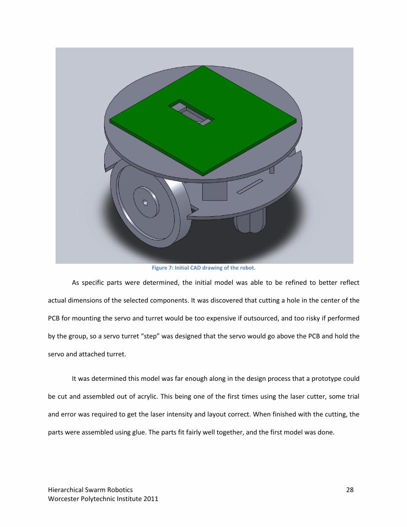
Figure 7: Initial CAD drawing of the robot.
As specific parts were determined, the initial model was able to be refined to better reflect
actual dimensions of the selected components. It was discovered that cutting a hole in the center of the
PCB for mounting the servo and turret would be too expensive if outsourced, and too risky if performed
by the group, so a servo turret “step” was designed that the servo would go above the PCB and hold the
servo and attached turret.
It was determined this model was far enough along in the design process that a prototype could
be cut and assembled out of acrylic. This being one of the first times using the laser cutter, some trial
and error was required to get the laser intensity and layout correct. When finished with the cutting, the
parts were assembled using glue. The parts fit fairly well together, and the first model was done.
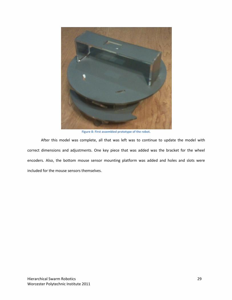
Hierarchical Swarm Robotics 29 Worcester Polytechnic Institute 2011
Figure 8: First assembled prototype of the robot.
After this model was complete, all that was left was to continue to update the model with
correct dimensions and adjustments. One key piece that was added was the bracket for the wheel
encoders. Also, the bottom mouse sensor mounting platform was added and holes and slots were
included for the mouse sensors themselves.
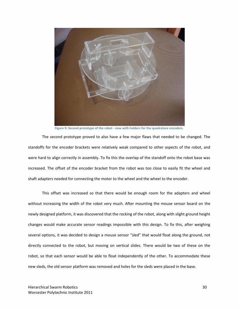
Hierarchical Swarm Robotics 30 Worcester Polytechnic Institute 2011
Figure 9: Second prototype of the robot - now with holders for the quadrature encoders.
The second prototype proved to also have a few major flaws that needed to be changed. The
standoffs for the encoder brackets were relatively weak compared to other aspects of the robot, and
were hard to align correctly in assembly. To fix this the overlap of the standoff onto the robot base was
increased. The offset of the encoder bracket from the robot was too close to easily fit the wheel and
shaft adapters needed for connecting the motor to the wheel and the wheel to the encoder.
This offset was increased so that there would be enough room for the adapters and wheel
without increasing the width of the robot very much. After mounting the mouse sensor board on the
newly designed platform, it was discovered that the rocking of the robot, along with slight ground height
changes would make accurate sensor readings impossible with this design. To fix this, after weighing
several options, it was decided to design a mouse sensor “sled” that would float along the ground, not
directly connected to the robot, but moving on vertical slides. There would be two of these on the
robot, so that each sensor would be able to float independently of the other. To accommodate these
new sleds, the old sensor platform was removed and holes for the sleds were placed in the base.

Hierarchical Swarm Robotics 31 Worcester Polytechnic Institute 2011
Figure 10: Enclosure (sled) for a single mouse sensor.
Initially, the plan was to have springs push the sleds down onto the ground for a solid
connection with the floor. However, since the robots are very light weight, springs would reduce the
traction of the drive wheels too much. Also, the springs would get caught on the bolts they were
intended to ride on and would not allow for smooth floating. However the good news was that the
mouse sleds floated well without springs because of the weight of the sleds and size of the holes in the
main platform.

Hierarchical Swarm Robotics 32 Worcester Polytechnic Institute 2011
Figure 11: The final, fully assembled robot with encoders, wheels, PCB, and sensor turret.
Due to electrical issues described later, the mouse sensor sleds were not used in the final
design. The sleds were removed from the design, leaving encoders as the only form of localization.
Above is a picture of one of the four final assembled robots. A minor fix was added post-design to fix
encoder issues, which can be seen on the outer side of the robot. All parts were installed on the four
robots, including the PCB, wheels, motors, encoders, servo, and turret with sensors.
Electrical Design This section describes the electrical design choices made when constructing the robots. All
electrical PCB design was completed in the free version of Eagle.

Hierarchical Swarm Robotics 33 Worcester Polytechnic Institute 2011
Queen and Worker
The top levels of the swarm (the queen and the workers) are based mostly in software rather
than hardware so it is simpler to discuss their reduced hardware requirements first. Due to time and
budget constraints, the worker became entirely virtual and could be running on the same laptop as the
queen. However, the electrical design still reflects the original goal of having worker level robots in the
physical world and therefore much of this section describes how the worker would run provided it was
not virtualized.
Design Requirements
The queen requires the most processing power out of any level of the swarm. However, there is
no reason the queen needs to be mobile so its role can be fulfilled by a laptop. The worker has similar
requirements to the queen however less processing power is required and mobility was originally
desired. For this reason the BeagleBoard was chosen for its large online community support, small size
and relatively low power consumption. The BeagleBoard also has the I/O capabilities to be able to
directly communicate with sensors if needed. However, it was decided that the simplest method would
be to have a separate board (dubbed the MobileBoard) used for direct sensor communication and
motor control. The MobileBoard would be capable of reading and interpreting the sensors to provide
the BeagleBoard with any information needed. This design allows for the BeagleBoard to concentrate
solely on high level processing and allow low level control to be offloaded onto another system.
MobileBoard
The MobileBoard serves as the main control platform for the scouts and was intended to serve
as a method of low level hardware control for the workers. As mentioned before, when the workers
became virtual, parts of the design became vestigial, however their original purpose is discussed below.
Another component that was eventually removed from the project was the detection of candles but
again, they are discussed in terms of how they were intended to be used.
Hierarchical Swarm Robotics 34 Worcester Polytechnic Institute 2011
Design Requirements
The low level control board of the swarm had several design requirements which affected the
choice of electrical components. The robot would be battery powered so steps were taken to attempt
to conserve power. Another requirement was that the robot would be able to perform its own
localization which would require a non-trivial amount of processing power as well as I/O peripherals to
communicate with various sensors. The robot would also have to relay findings to its parent which
would require wireless communication. In order for the robot to be able to move, motor driver circuitry
was needed. This could take the form of either a DAC (Digital to Analog Converter) or H-Bridge.
Another design requirement was that it could detect both physical objects and “heat” (which for
practical reasons took the form of an IR beacon rather than an actual heat source). The final design
requirement was that the same board could be used for low level motor control/sensor interfacing for
the worker or used as the main control board for the scout.
Power Supplies
The decision was made early on that one of the easiest ways to conserve battery life was to use
a switching regulator rather than a linear one. A switching regulator works by essentially generating a
PWM signal whose duty cycle is adjusted so that the RMS voltage of the square wave is equal to the
desired output voltage. To power the MobileBoard, the desired outputs were 5V and 3.3V (the
operating voltages of the components used) and the input voltage ranged between 7.5V for two fully
charged batteries to as low as 6V for two nearly dead ones. The use of switching regulator dramatically
improves the efficiency of the circuit, due to the fact that a switching regulator operates transistors in
either a fully on or fully off state resulting in over 90% efficiency. In contrast, a linear regulator simply
dissipates excess voltage (or more accurately power because current is passing through the regulator as
well) as heat and the efficiency is determined only by the ratio of output to input voltages. For a fully
charged set of batteries, this would be 5V/7.5V or 66% efficient.

Hierarchical Swarm Robotics 35 Worcester Polytechnic Institute 2011
Care was also taken in ensuring that power supplies were adequately filtered and that grounds
were separated. In order to reduce the effects of noise on the circuit, the main 5V and 3.3V supplies
were split in to power, digital, and analog sections. Power sections received only minimal filtering in the
form of a capacitor on the output of the switching regulator to handle brief spikes in current draw from
a motor. The digital sections were filtered through an LC circuit to form a low pass filter to both remove
some of the ripple voltage created as a byproduct of a switching regulator and help protect against
potential voltage surges created by the back EMF of a motor. The analog sections received an additional
filter in order to create a voltage source as clean as possible for the components which would be most
sensitive to noise. A similar practice was done for grounding. Any high current component was
connected to power ground, digital components were connected to digital ground, and analog
components were connected to analog ground. All three grounds were connected at only a single point
so that any noise induced in the ground by either power or digital components would not have adverse
effects on analog components such as an ADC (Analog to Digital Converter).
Motor Control
In order for the robot to be able to move it is a requirement that the microcontroller needs to
have a method for controlling the speed of a motor. The motor control would be best accomplished
with an H-bridge circuit as this can operate without the use of a split power supply and is more efficient
than a linear DAC. A dual H-Bridge IC (TI’s SN754410) was selected with a max output current capacity
of 1A which exceeded the maximum of 600mA draw from a single motor. Since a motor behaves similar
to an inductor, when the H-Bridge disables the output channel (i.e. when the controlling PWM signal is
low) the inductance of the motor will not allow for current to stop instantaneously causing a very large
voltage surge on one of the motor terminals likely damaging the H-Bridge in the process. In order to
protect against this, schottky diodes were placed at both terminals of each motor which would become
forward biased and conduct whenever either terminal exceeded 5V or fell below 0V. The reason

Hierarchical Swarm Robotics 36 Worcester Polytechnic Institute 2011
schottky diodes were selected was for their fast recovery time allowing them to become conductive
before the voltage spike caused by the motor became too high.
Object and Heat Detection
Object and heat detection are best accomplished by separate sensors. A sharp IR rangefinder
works well for detecting a range to an object and an IR phototransistor operating on a different
wavelength is used for detecting “heat” or in this case, an IR emitter on the same wavelength as the
detector. Since the IR rangefinder and phototransistor operate on separate wavelengths, the two do
not interfere with each other. When used simultaneously, the IR rangefinder can accurately measure
the distance to a given object and the heat sensor can be used to detect if the object observed by the
rangefinder is a virtual heat source or simply an ordinary wall. The IR heat detector could also be used
for a second purpose. By modulating the IR emitter as a square wave with a preset duty cycle the same
circuitry for a virtual candle can be used as an IR beacon that a robot can recalibrate against in order to
correct for odometry drift (assuming the location of the IR beacon is known). This feature was never
implemented however the hardware still supports it.
Localization Sensors
Tracking the position of an indoor robot accurately is not a simple task. With GPS unusable
indoors there is little existing infrastructure which can be used for accurate positioning. Wi-Fi
localization can narrow down the position to within the range of a single access point however this is
not nearly accurate enough for this application. Odometry requires no additional deployment and has
very good short term accuracy but suffers from uncorrectable drift over time causing long term accuracy
problems. Every other localization technique designed for indoor use was simply too expensive for this
project. One of the more expensive is the Stargazer system which relies on observing predefined
markings on the ceiling with a camera and by observing the position and orientation of those markings

Hierarchical Swarm Robotics 37 Worcester Polytechnic Institute 2011
could calculate the position of a robot. This system however would require putting a $900 camera on
each robot (more than the cost of every other component combined).
With this in mind, the final choice for sensors were encoders attached to the drive wheels and
optical mouse sensors on either side of the robot to track ground movement relative to the robot. The
use of multiple sensors allows for redundancy so if one sensor were to receive a bad reading the other
would likely still be correct. In that way, the amount of drift experienced can be reduced (although not
eliminated). The encoders directly measure angular displacement of the wheels and work well for being
used as feedback for a PD velocity controller. The encoders are prone to wheel slip but otherwise are
unlikely to miss any counts while the wheel is moving. The optical mouse sensors have the advantage of
being immune to wheel slip as they measure the displacement against the ground directly however they
are able to occasionally misjudge the actual displacement and any drift experienced is not able to be
corrected without the help of another sensor. The mouse sensors were found to be unusable for this
project due to strict mounting tolerance which could not be achieved. Again however, the support for
the sensors still exists in the hardware and software.
Wireless Communication
When a parent robot wishes to issue a command to a child or a child wishes to relay information
back to a parent it must have a way of transmitting this information. Several wireless protocols exist
which are capable of performing this function. 802.11 Is widely used for wireless internet access and
supports high data rates and good range at the cost of consuming a relatively large amount of power.
Bluetooth supports mid range data rates (enough for audio streaming) and has a limited range but
consumes less power than an 802.11 transceiver. The final major protocol which was studied as a
potential candidate was ZigBee which is designed for low data rates, extremely low power, and ranges
comparable to and possibly exceeding 802.11. Digi International has created XBee modules which use
the ZigBee protocol to allow for transmission of data from point to point through the ZigBee mesh
Hierarchical Swarm Robotics 38 Worcester Polytechnic Institute 2011
network. The XBee modules proved to be the simplest to use, lowest power, and most cost effective for
this swarm. Therefore, the choice was made to use the XBee modules for wireless communication.
Processor Selection
With all of the peripherals chosen it was then possible to begin selecting candidates for a
microcontroller to serve as the main processor for the MobileBoard. The microcontroller needed to
have a variety of I/O capabilities to support communication over UART for the XBee module, SPI for the
encoder counter and optical mouse sensors, and it also needed the ability to read analog values with an
ADC to use the IR rangefinders. The microcontroller also would be responsible for updating its position
very frequently which requires a reasonable amount of processing power. Finally, the processor must
consume low amounts of power in order to conserve battery life. There were two major candidates for
the microcontroller: TI’s MSP430F5438 and Atmel’s Xmega128A1. The MSP430 is known for its
extremely low power consumption and had the I/O peripherals required to communicate with every
sensor. The Xmega’s power consumption is higher however it has a faster clock speed as well as an
extensive set of peripherals. Both processors were compatible with μC/OS-II (a real time operating
system or RTOS, which will be explained further in a later section) having both the RAM and flash
memory required.

Hierarchical Swarm Robotics 39 Worcester Polytechnic Institute 2011
MSP430F5438 Xmega128A1
Clock Speed 16MHz 32MHz with DFLL for increased accuracy
RAM 16kB 8kB
Flash Memory 256kB 128kB
Timers 3 16-bit 8 16-bit
ADC 12-bit 2 12-bit
DMA 4 channel 4 channel
SPI 8 4 Master/Slave + 8 Master Only
UART 4 8
Tools Provided Free limited IDE’s available
AVR Studio provided for free with no limitations.
Figure 12: Comparison of the MSP430F5438 and the Xmega128A1.
The table shows that although the MSP430 has more RAM and code space, the Xmega is the
faster chip and the clock is also able to be automatically calibrated for increased timer accuracy. Speed
and ease of use were the deciding factors because having more RAM or code space than needed does
not yield better performance. Having more processing speed on the other hand simply allows for faster
polling of the sensors and a faster interrupt response time. The faster CPU would also be useful to
offset the fact that neither processor had an FPU (Floating Point Unit) so all floating point calculations
must be emulated in software.
Circuit Design
Circuit design proved to be a difficult task as no member of the group had any previous
experience with PCB design. Therefore, there was a steep learning curve involved in getting the
schematics for the MobileBoard completed. In addition to this problem, there was also the issue of
having several devices with different operating voltages. The BeagleBoard intended to be used by the
mid level robots used 1.8V I/O levels but the Xmega used 3.3V levels. The IR rangefinder and encoders

Hierarchical Swarm Robotics 40 Worcester Polytechnic Institute 2011
worked on 5V however the encoder counting IC ran on 3.3V and the ADC in the Xmega uses a 1V
reference voltage. Clearly a solution was needed for converting many of the logic levels used. This
solution came in the form of a simple circuit involving a single N-Channel MOSFET and two pull up
resistors. The circuit used is shown below.
Figure 13: Circuit of the N-Channel MOSFET and two pull up resistors.
This circuit allows for bidirectional logic translation between any two levels (V1 and V2). This
circuit would have been used to allow the Xmega to communicate with the BeagleBoard as well as for
the Xmega to use a PWM signal to control the 5V servo. In order to solve the problem of interfacing the
5V encoders with the 3.3V encoder counter, a simple voltage divider was used. The voltage divider
stepped the 5V encoder pulses down to approximately 3.3V. This approach was used again to ensure
that the output of the IR rangefinder remained within the 0-1V range detectable by the ADC of the
Xmega
Another important feature added to the MobileBoard was the ability to selectively enable or
disable the IR rangefinders and servo motor. Both of these devices would not be used while driving and
it therefore was deemed prudent to disable them to prolong the life of the batteries. The enable circuit
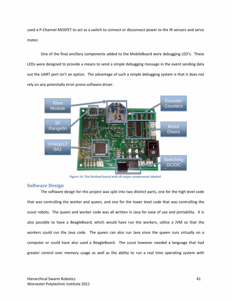
Hierarchical Swarm Robotics 41 Worcester Polytechnic Institute 2011
used a P-Channel MOSFET to act as a switch to connect or disconnect power to the IR sensors and servo
motor.
One of the final ancillary components added to the MobileBoard were debugging LED’s. These
LEDs were designed to provide a means to send a simple debugging message in the event sending data
out the UART port isn’t an option. The advantage of such a simple debugging system is that it does not
rely on any potentially error prone software driver.
Figure 14: The finished board with all major components labeled.
Software Design The software design for this project was split into two distinct parts, one for the high level code
that was controlling the worker and queen, and one for the lower level code that was controlling the
scout robots. The queen and worker code was all written in Java for ease of use and portability. It is
also possible to have a BeagleBoard, which would have run the workers, utilize a JVM so that the
workers could run the Java code. The queen can also run Java since the queen runs virtually on a
computer or could have also used a BeagleBoard. The scout however needed a language that had
greater control over memory usage as well as the ability to run a real time operating system with
Xmega128A1
Processor
Encoder Counters
Motor Divers
Switching DC/DC
Regulators
IR Rangefinder Ports
Xbee Module
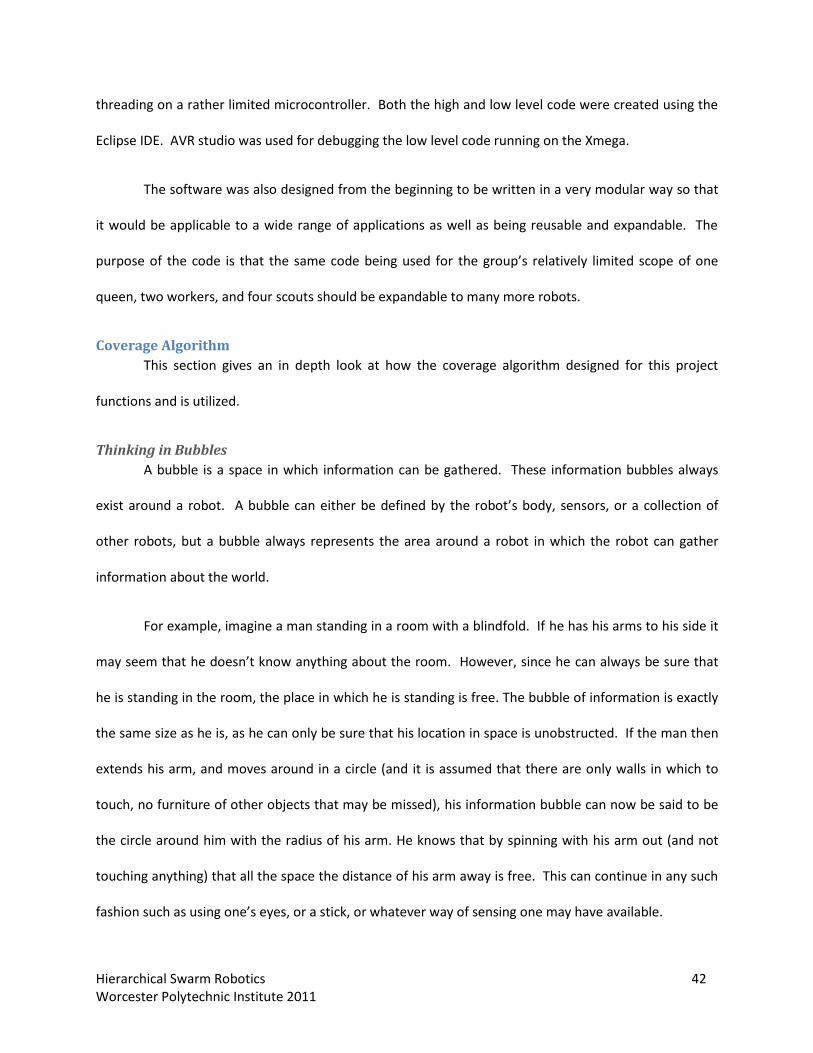
Hierarchical Swarm Robotics 42 Worcester Polytechnic Institute 2011
threading on a rather limited microcontroller. Both the high and low level code were created using the
Eclipse IDE. AVR studio was used for debugging the low level code running on the Xmega.
The software was also designed from the beginning to be written in a very modular way so that
it would be applicable to a wide range of applications as well as being reusable and expandable. The
purpose of the code is that the same code being used for the group’s relatively limited scope of one
queen, two workers, and four scouts should be expandable to many more robots.
Coverage Algorithm
This section gives an in depth look at how the coverage algorithm designed for this project
functions and is utilized.
Thinking in Bubbles
A bubble is a space in which information can be gathered. These information bubbles always
exist around a robot. A bubble can either be defined by the robot’s body, sensors, or a collection of
other robots, but a bubble always represents the area around a robot in which the robot can gather
information about the world.
For example, imagine a man standing in a room with a blindfold. If he has his arms to his side it
may seem that he doesn’t know anything about the room. However, since he can always be sure that
he is standing in the room, the place in which he is standing is free. The bubble of information is exactly
the same size as he is, as he can only be sure that his location in space is unobstructed. If the man then
extends his arm, and moves around in a circle (and it is assumed that there are only walls in which to
touch, no furniture of other objects that may be missed), his information bubble can now be said to be
the circle around him with the radius of his arm. He knows that by spinning with his arm out (and not
touching anything) that all the space the distance of his arm away is free. This can continue in any such
fashion such as using one’s eyes, or a stick, or whatever way of sensing one may have available.

Hierarchical Swarm Robotics 43 Worcester Polytechnic Institute 2011
The same applies for a robot. If all it has are bump sensors, its bubble is defined by its location
in space. It knows that all the space taken up by its body is not in fact unknown, but is instead free. If
the robot has an IR sensor, it knows that it can gather information anywhere from 10 – 80cm in radius
(with the IR sensors used on this project) from itself.
The bubble concept is a way of abstracting a means of gathering information such that within
the context of this swarm, two robots of different levels have no reason to know how information is
being obtained, simply that they can request information from a given bubble, and then have that
information returned to them. For the scouts, they know their bubble size based off of the range of the
IR sensor. At startup, the upper levels of the swarm send a request for information to their children.
The information packet that comes back contains all the needed information, which is the current
location of the child and its minimum and maximum bubble size. For example, when a scout joins with a
worker it will inform the worker that it can be asked for information anywhere between 10cm away and
80cm away. When the worker asks for information, it does so by communicating the idea of “give me
information in a X cm radius around yourself.” In that way, the worker can receive information from
the scout without ever having to worry about where it comes from or how it is gathered.
The same concept can then be further abstracted to the next level up in the swarm. A worker’s
information bubble is defined by the space in which all of its scouts can gather information. At a
minimum, this size is considered to be the minimum size for all the scouts to fit and scan with their own
minimum radius around the worker. The maximum bubble for the worker is considered to be the
maximum communication range of the hardware that the worker is using to communicate. Due to this,
the maximum bubble size of the worker will vary based on hardware implementation.
However, the important fact is that the queen does not care how the worker gathers
information; all the queen cares about is the size of the bubble the worker can gather. The queen is

Hierarchical Swarm Robotics 44 Worcester Polytechnic Institute 2011
unsure if the worker has children itself, if it is doing any scanning with sensors, or if it is simply driving
around the entire space it has been given. More importantly, the queen does not care. All the queen is
concerned with is that if it asks the worker for information around it, the worker will in some way gather
that information and report it back to its parent when complete.
Figure 15: Three different ways of gathering information in a bubble. Using a sharp IR sensor (left), driving to all points in the
bubble (center), and breaking the bubble up further for children (right).
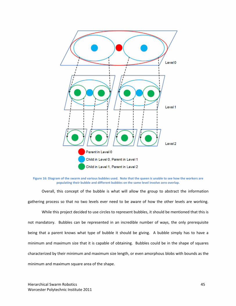
Hierarchical Swarm Robotics 45 Worcester Polytechnic Institute 2011
Figure 16: Diagram of the swarm and various bubbles used. Note that the queen is unable to see how the workers are populating their bubble and different bubbles on the same level involve zero overlap.
Overall, this concept of the bubble is what will allow the group to abstract the information
gathering process so that no two levels ever need to be aware of how the other levels are working.
While this project decided to use circles to represent bubbles, it should be mentioned that this is
not mandatory. Bubbles can be represented in an incredible number of ways, the only prerequisite
being that a parent knows what type of bubble it should be giving. A bubble simply has to have a
minimum and maximum size that it is capable of obtaining. Bubbles could be in the shape of squares
characterized by their minimum and maximum size length, or even amorphous blobs with bounds as the
minimum and maximum square area of the shape.
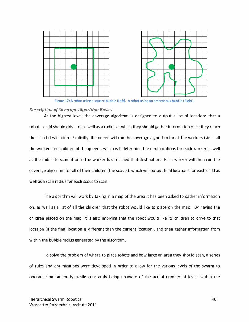
Hierarchical Swarm Robotics 46 Worcester Polytechnic Institute 2011
Figure 17: A robot using a square bubble (Left). A robot using an amorphous bubble (Right).
Description of Coverage Algorithm Basics
At the highest level, the coverage algorithm is designed to output a list of locations that a
robot’s child should drive to, as well as a radius at which they should gather information once they reach
their next destination. Explicitly, the queen will run the coverage algorithm for all the workers (since all
the workers are children of the queen), which will determine the next locations for each worker as well
as the radius to scan at once the worker has reached that destination. Each worker will then run the
coverage algorithm for all of their children (the scouts), which will output final locations for each child as
well as a scan radius for each scout to scan.
The algorithm will work by taking in a map of the area it has been asked to gather information
on, as well as a list of all the children that the robot would like to place on the map. By having the
children placed on the map, it is also implying that the robot would like its children to drive to that
location (if the final location is different than the current location), and then gather information from
within the bubble radius generated by the algorithm.
To solve the problem of where to place robots and how large an area they should scan, a series
of rules and optimizations were developed in order to allow for the various levels of the swarm to
operate simultaneously, while constantly being unaware of the actual number of levels within the

Hierarchical Swarm Robotics 47 Worcester Polytechnic Institute 2011
swarm, or the knowledge of “neighbors” within a robots own level. The rules and optimizations for the
swarm are discussed in detail next.
Greedy Algorithm Vs. Optimal Solution
Originally when the Coverage Algorithm was still in its relative infancy a dynamic programming
solution was perused that would generate the true optimal placement of a child’s bubble. However, it
was soon discovered that this was significantly less than trivial and was in fact an intractable problem.
Once this was determined, it was also found that a greedy approach to the same problem provided a
good approximation of the optimal solution that the dynamic programming solution would have
provided. For those reasons, it was decided that a greedy approach would be used in order to place the
robots on the map. The greedy approach would simply select the best locations for the robots given a
set of criteria and a way to rank all the possible locations.
Rules of the Coverage Algorithm
The rules of the coverage algorithm are the guiding principles of how the algorithm will run.
While the optimizations are designed to allow the algorithm to complete in a faster or more efficient
manner, the rules are needed in order to allow the algorithm to complete at all. Each rule has a specific
function that was determined by studying how the robots would behave in the real world. Below is a
statement of each of the rules, as well as its justification and real world significance.
Rule 1: Bubbles Generated by the Coverage Algorithm Cannot Overlap
The first rule of the coverage algorithm is the most crucial to the running of actual robots in a
physical environment. The rule simply states that the bubbles generated by the coverage algorithm
cannot overlap. The reasoning behind this is that the children of a parent will only know or gather
information from within that radius and by ensuring that they do not overlap, it allows for a few key
facts to be assumed. It allows a robot to know that if its children do not overlap, then its children’s

Hierarchical Swarm Robotics 48 Worcester Polytechnic Institute 2011
children will also not overlap, etc. If the bubbles could overlap, then a robot’s “grandchildren”
(children’s children) could collide due to the fact that they are mapping the same region.
Figure 18: A sample of how the bubbles might be placed by the coverage algorithm. Note that none of the bubble centers
are in unknown space and none of the bubbles overlap.
From this rule also stem a few implications about how the robots gather information
themselves. The main implication is that robots should throw out any information that is obtained
about a space outside the given bubble. For example if a worker is told to scan a given area, and then
placed a scout (one of its children) in such a way so that the scout scans outside of the bubble of the
worker, the information about the area outside of where the worker was told to scan will be
disregarded. The reasoning behind this is that, as stated above, the worker can only be sure about the
information it is gathering inside its own bubble. If the scout had seen an object outside the workers
bubble and reported it back, the worker has no way of knowing if it is an object, robot, or something
entirely different such as sensor interference.

Hierarchical Swarm Robotics 49 Worcester Polytechnic Institute 2011
Figure 19: Depiction of a level 2 robot (bubble shown in green) scanning within a level 1 robot’s bubble (shown in blue). Since the level 2 robot’s bubble extends beyond the Level 1 robot’s bubble, none of the information outside the level 1
robot’s bubble (shown as the grey squares) will be saved.
The second implication is that the robot can only place its children within the bubble (note that
the bubble may extend beyond the bubble of the assigning robot but the data will be thrown away) it
has been assigned. Following the same example as above, the worker cannot place any of its scouts
outside of the bubble assigned to it by the queen. Again for the same reasons above, this is because the
worker would have no way of knowing what may lie just outside its bubble, and may end up driving the
scout into another robot or even off a cliff.
Figure 20: Valid placement of children by the coverage algorithm (left), invalid placement by the coverage algorithm (right).

Hierarchical Swarm Robotics 50 Worcester Polytechnic Institute 2011
Rule 2: Coverage Algorithm Cannot Route a Robot through Unknown Space
The second rule for the coverage algorithm has to do with placing the bubbles while taking into
account the unknown certainty of un-scanned space. The second rule states that the robot must be
placed in known space and be able to reach that location without traveling through unknown space. The
reasoning was that if a parent tells its child to drive and scan in unknown space, it has no actual way of
knowing if the child is capable of reaching its destination.
Rule 3: Bubbles Must Follow the Assigned Minimum and Maximum Size
The final rule of the coverage algorithm is a bit more of a common sense implementation. A
bubble placed by the coverage algorithm must comply with the minimum and maximum bubble sizes
that were given to the parent by the child. The reason for this is simply because the child has reported
that for whatever reason the bubble it is assigned must conform to the specified minimum and
maximum and asking the child to exceed those limits may not be possible for the child to do.
Heuristics of the Coverage Algorithm
These heuristics were determined to be best for this specific usage of the coverage algorithm.
1) Bubbles Must be the Same Amount of “Work”
The first heuristic that was determined for the successful running of a swarm in the real world is
that bubbles placed by the coverage algorithm should take the same amount of effort to scan. The
amount of work to uncover the area should be reduced down to a simple and comparable factor. Some
examples of expenditures could be time or energy. The heuristic that was used for this project was that
the bubbles must be the same size. This simple heuristic works well for a swarm where the hierarchy is
“balanced” (all nodes on a given level have the same number of children) and where all of the scouts use
the same sensors to scan an area. One example where this heuristic is less optimal would be where the
queen tells two workers to scan the same size area but one worker has two scouts to work with and the
other has five. Clearly the worker with the larger number of scouts can complete the same task more
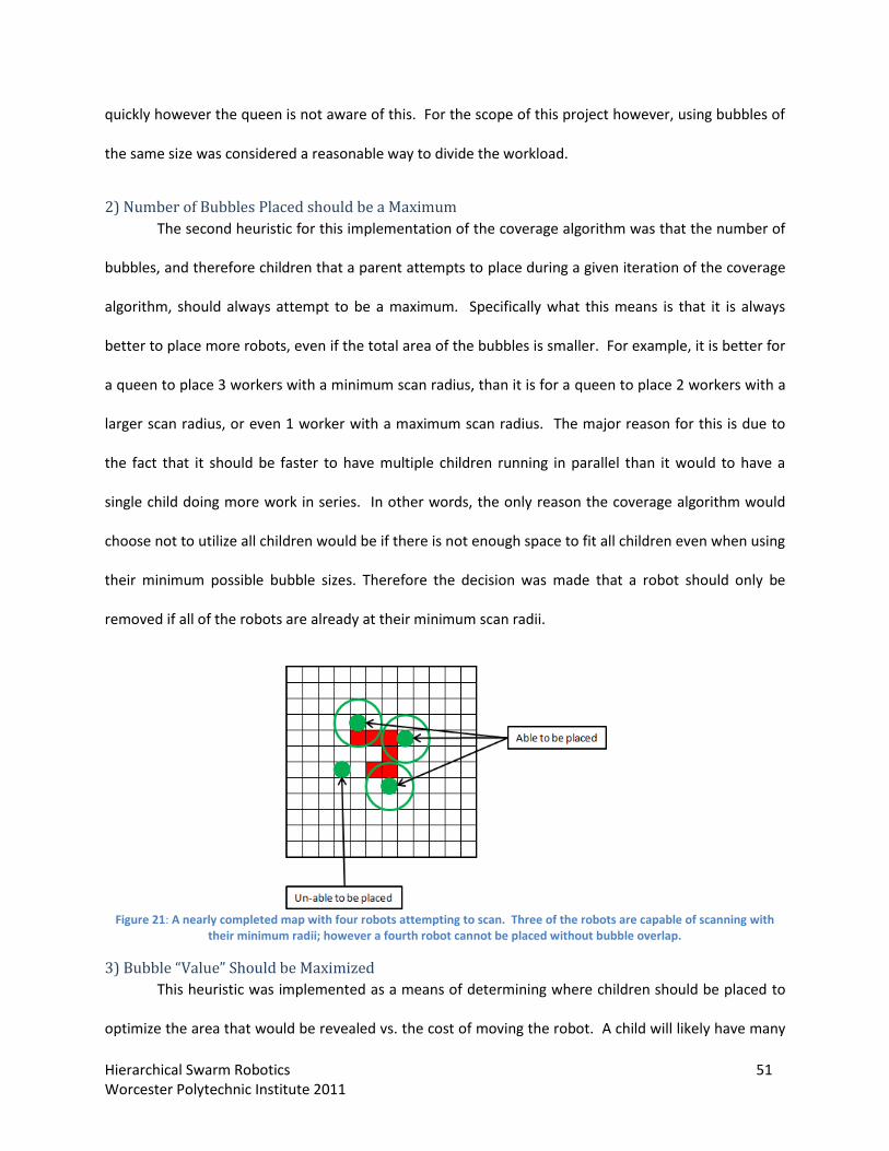
Hierarchical Swarm Robotics 51 Worcester Polytechnic Institute 2011
quickly however the queen is not aware of this. For the scope of this project however, using bubbles of
the same size was considered a reasonable way to divide the workload.
2) Number of Bubbles Placed should be a Maximum
The second heuristic for this implementation of the coverage algorithm was that the number of
bubbles, and therefore children that a parent attempts to place during a given iteration of the coverage
algorithm, should always attempt to be a maximum. Specifically what this means is that it is always
better to place more robots, even if the total area of the bubbles is smaller. For example, it is better for
a queen to place 3 workers with a minimum scan radius, than it is for a queen to place 2 workers with a
larger scan radius, or even 1 worker with a maximum scan radius. The major reason for this is due to
the fact that it should be faster to have multiple children running in parallel than it would to have a
single child doing more work in series. In other words, the only reason the coverage algorithm would
choose not to utilize all children would be if there is not enough space to fit all children even when using
their minimum possible bubble sizes. Therefore the decision was made that a robot should only be
removed if all of the robots are already at their minimum scan radii.
Figure 21: A nearly completed map with four robots attempting to scan. Three of the robots are capable of scanning with
their minimum radii; however a fourth robot cannot be placed without bubble overlap.
3) Bubble “Value” Should be Maximized
This heuristic was implemented as a means of determining where children should be placed to
optimize the area that would be revealed vs. the cost of moving the robot. A child will likely have many

Hierarchical Swarm Robotics 52 Worcester Polytechnic Institute 2011
different possible locations where it could be placed however some of them would uncover very little
area or may force the robot to drive a great distance.
Figure 22: Picture of various locations a robot could move to and scan with a radius of 3 cells and their corresponding value. The location marked 35 is highest value because it scanning at that location would uncover a high number of cells without
much driving. The locations marked 25 and 15 are progressively lesser value due to the fact that they uncover a similar number of cells however require significantly more travel. The last location marked 2 is lowest value due to the fact that it is
close, however scanning there would not uncover a large number of cells.
The simplest method to perform a cost-benefit analysis is shown in the equation below.
Here V represents the value of a bubble, C represents the number of cells which the bubble would
reveal, and D represents the required distance for a robot to drive to begin scanning. Note that the
value for C is not simply the number of cells contained within the bubble, as only cells which are not
already scanned can be revealed. It is also worth noting that depending on the obstacles in the bubble,
not every cell is guaranteed to be scanned when the child completes its bubble. However, since there is
no way of knowing this, the value function is optimistic and assumes the best case scenario that all cells
in a bubble that are un-scanned will be revealed. The parameters α and β are arbitrary constants which
can be tuned to reflect the value gained by uncovering more cells or the value lost by driving more.

Hierarchical Swarm Robotics 53 Worcester Polytechnic Institute 2011
In this particular implementation of the coverage algorithm, good results have been achieved by
setting the cells uncovered constant (α) to be 1, and the distance driven constant (β) to be 3. What this
means is that for every cell driven, 3 additional cells need to be uncovered to make the extra time spent
driving worth the effort. In the event that two bubbles are evaluated to the same number, no
preference is given between the two and the selection is more or less at random.
4) Midpoint of Bubble must Border Known and Unknown Space
This heuristic is designed to reduce the amount of time it takes to complete an iteration of the
coverage algorithm. Although the value metric discussed will work for determining the value of any
bubble placement (including ones which place the bubble in entirely known space), it is a waste of
resources to attempt to place bubbles in a location that will definitely not be optimal. Rather than
obtaining potential value of a bubble at every possible location a robot could drive to, the requirement
is added that a bubble must be placed somewhere that borders unknown space. This will ensure that at
least one cell will be uncovered when the scan is performed and eliminates all of the useless bubble
placements.
Figure 23: Picture of robot scanning in known space, uncovering no new information (left). If the robot is placed on the
boarder of known and unknown space it is a guarantee that at least one new cell of information will be uncovered (right).
In-depth Description of the Coverage Algorithm
Pseudocode Description
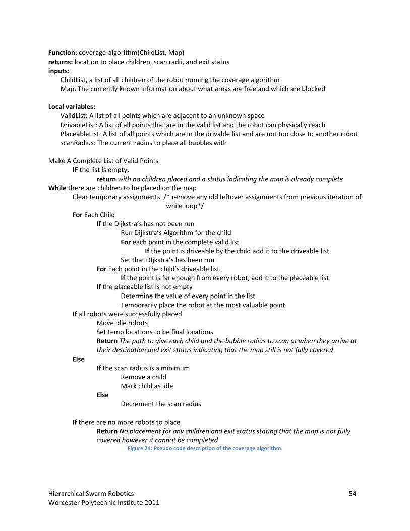
Hierarchical Swarm Robotics 54 Worcester Polytechnic Institute 2011
Function: coverage-algorithm(ChildList, Map) returns: location to place children, scan radii, and exit status inputs:
ChildList, a list of all children of the robot running the coverage algorithm Map, The currently known information about what areas are free and which are blocked
Local variables:
ValidList: A list of all points which are adjacent to an unknown space DrivableList: A list of all points that are in the valid list and the robot can physically reach PlaceableList: A list of all points which are in the drivable list and are not too close to another robot scanRadius: The current radius to place all bubbles with
Make A Complete List of Valid Points IF the list is empty,
return with no children placed and a status indicating the map is already complete While there are children to be placed on the map
Clear temporary assignments /* remove any old leftover assignments from previous iteration of while loop*/
For Each Child If the Dijkstra’s has not been run Run Dijkstra’s Algorithm for the child For each point in the complete valid list If the point is driveable by the child add it to the driveable list Set that DIjkstra’s has been run For Each point in the child’s driveable list If the point is far enough from every robot, add it to the placeable list If the placeable list is not empty Determine the value of every point in the list Temporarily place the robot at the most valuable point If all robots were successfully placed Move idle robots Set temp locations to be final locations
Return The path to give each child and the bubble radius to scan at when they arrive at their destination and exit status indicating that the map still is not fully covered
Else If the scan radius is a minimum Remove a child Mark child as idle Else Decrement the scan radius If there are no more robots to place
Return No placement for any children and exit status stating that the map is not fully covered however it cannot be completed
Figure 24: Pseudo code description of the coverage algorithm.

Hierarchical Swarm Robotics 55 Worcester Polytechnic Institute 2011
Although the pseudocode appears quite complicated, the process can be described in English
without too much difficulty. Following the rules and heuristics stated previously, the algorithm attempts
to place all children at their maximum scan radius without allowing any two bubbles to overlap. If the
bubbles do not overlap, the children can be placed successfully and the algorithm returns the path to
assign them as well as the scanning radius to use. If the bubbles cannot be placed without overlapping,
the algorithm retries placing the children using smaller scan radii. If the scan radius is at a minimum, the
algorithm will remove a child and check if the overlap has been removed. If it is forced to remove all
children the algorithm determines it cannot obtain any more coverage of the map.
Although the cursory explanation of the algorithm is sufficient for understanding the general
process for placing children, it is not descriptive enough to explain some of the details implied in the
pseudocode that help improve runtimes. From the beginning, the first step is simply to generate a list of
every cell which is adjacent to an un-scanned cell (for reasons stated in the heuristics section above).
This is known as the valid list. If this list is empty, it means that there are no cells in the map which are
not scanned so the map has been entirely revealed. Therefore, the coverage algorithm does not need to
do anything because there is nothing left to cover.
If there are still points that border unknown space the coverage algorithm begins attempting to
place children. Dijkstra’s algorithm [18] is run on every child to find the optimal path to every cell in the
map (if any path is possible). This can be used to eliminate points from the valid list that are not actually
reachable by the robot. A new list is generated that contains only points that are both valid and
reachable by the robot known as the drivable list.

Hierarchical Swarm Robotics 56 Worcester Polytechnic Institute 2011
Figure 25: Picture of a map showing locations that are valid and drivable, as well as valid and un-drivable.
The drivable list can then be reduced even further by removing points which conflict with
existing bubbles. This removal stops the algorithm from placing bubbles which can overlap each other.
The algorithm builds what is known as the placeable list which contains all points that were in the
drivable list and do not cause any overlap among existing bubbles. The reason for continuing to reduce
this list so many times is because this results in the smallest number of points to evaluate for placement.
The evaluation process is the function mentioned earlier (V= αC – βD) and although it is not incredibly
complicated, computing the value for C (the number of cells which a robot would uncover) does require
enough calculations that it is prudent not to waste time computing the value for points which are in the
valid list but the child could not actually drive to or be placed at due to bubble overlap.
When the placeable list has been built for a child, the algorithm computes the value for every
bubble which could be created at a point in the placeable list and chooses the point that yields the
highest value. Once a child has been placed, the coverage algorithm repeats the entire process again for
the next child until all children are placed. Note that as stated earlier, if a child cannot be placed then
the algorithm restarts from the beginning attempting to place children using smaller bubbles. When the
bubbles cannot be made smaller, the algorithm instead removes a child.

Hierarchical Swarm Robotics 57 Worcester Polytechnic Institute 2011
A significant consequence of this is that if the algorithm is forced to restart, due to being unable
to place a child, it has effectively lost any progress made when placing the children and starts from
scratch. Therefore, it is important that the reduction steps taken to produce the placeable list are done
on a single child at a time rather than creating all valid points for all children, then reducing the list to
the drivable list for all children, then reducing to the placeable list for all children. If the latter approach
were taken, if the algorithm found that it could not place all children it would have wasted the effort of
performing all the list reduction steps. Alternatively, if the process is done in a different order where
the list is reduced down to the placeable list for child 1 before even populating the valid list for child 2,
as soon as a child is found to have an empty placeable list there is no need to continue attempting to
place any more children because it is known that at least one child cannot be placed with the current
scan radius. By using this fail-fast method the runtime of the algorithm is reduced significantly.
The last important function the coverage algorithm performs is “Move Idle Robots.” This deals
with the fact that if not all children are able to be placed; some of the children will not participate in
scanning with their siblings. However, the children may need to move out of the way to prevent them
from sitting inside another child’s bubble. “Move Idle Robots” simply checks to make sure that any
robot that has not been utilized by the algorithm is not in the way of any robots which will be given
bubbles to scan. If an idle robot is in the way, it is assigned a path that will move the robot out of the
way.
Other Interesting Features
The below sections describe specific aspects of the algorithm that were agreed as generally
interesting and unique. The details discussed here are not particularly related to the process the
algorithm uses as a whole, but the features described here were deemed interesting enough to mention
in this paper.
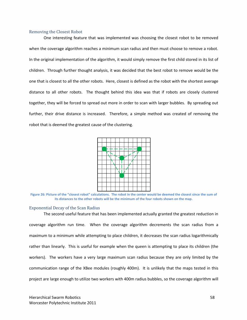
Hierarchical Swarm Robotics 58 Worcester Polytechnic Institute 2011
Removing the Closest Robot
One interesting feature that was implemented was choosing the closest robot to be removed
when the coverage algorithm reaches a minimum scan radius and then must choose to remove a robot.
In the original implementation of the algorithm, it would simply remove the first child stored in its list of
children. Through further thought analysis, it was decided that the best robot to remove would be the
one that is closest to all the other robots. Here, closest is defined as the robot with the shortest average
distance to all other robots. The thought behind this idea was that if robots are closely clustered
together, they will be forced to spread out more in order to scan with larger bubbles. By spreading out
further, their drive distance is increased. Therefore, a simple method was created of removing the
robot that is deemed the greatest cause of the clustering.
Figure 26: Picture of the “closest robot” calculations. The robot in the center would be deemed the closest since the sum of
its distances to the other robots will be the minimum of the four robots shown on the map.
Exponential Decay of the Scan Radius
The second useful feature that has been implemented actually granted the greatest reduction in
coverage algorithm run time. When the coverage algorithm decrements the scan radius from a
maximum to a minimum while attempting to place children, it decreases the scan radius logarithmically
rather than linearly. This is useful for example when the queen is attempting to place its children (the
workers). The workers have a very large maximum scan radius because they are only limited by the
communication range of the XBee modules (roughly 400m). It is unlikely that the maps tested in this
project are large enough to utilize two workers with 400m radius bubbles, so the coverage algorithm will

Hierarchical Swarm Robotics 59 Worcester Polytechnic Institute 2011
need to attempt to place the workers many times with smaller and smaller radii until both can be used.
Doing this linearly on a 20m x 20m map will take at least 390 decrements before both workers can fit
within the map (assuming 1m per decrement). In order to speed up the process, the radii were
decreased in an exponential manner where the next radius to try is 90% of the previous one. In the
previous example, rather than stepping through 400m, 399m, 398m, etc., the algorithm will try 400m,
360m, 324m, etc. This provided a good balance for quickly reducing the bubble size when needed
without having a low resolution of bubble sizes for smaller bubbles.
Move Idle Robots
Although the function that “move idle robots” provides was described earlier, this section
covers how it works in more detail. Once the coverage algorithm was finished placing as many as robots
as it could, it would check to see if any of the robots in its list were not told to scan. If there were any
robots that weren’t currently scanning, the algorithm would check if any of the robots were in conflict
(within the scan radius) of other robots that were being told to scan. If any of the idle robots were
within another robots radius, the coverage algorithm would then move those robots out of the way. By
moving the idle robot, it would no longer be sitting in the way of any other robot’s bubble or their drive
path.
The way this was performed was to come up with a list of all the points that were covered by a
scan of the other robots. That list was then expanded to include all points that any robot would drive
through while getting to their next location. Then, for each idle robot that iteration, the coverage
algorithm would spiral out from the idle robot’s current location in order to find the closest possible
location that was not in the list of conflicted points. Once the idle robot had a new home, that location,
and the path to reach it, was added to the list of conflict points so that no two idle robots were routed
to the same position. The spiral pattern was chosen in order to attempt to minimize overall drive
distance of the idle robots.

Hierarchical Swarm Robotics 60 Worcester Polytechnic Institute 2011
Finally, an addition was made so that any idle robots moving to new locations would be told to
move before the other children who were scanning. Moving them first was implemented because it was
unknown whether or not they were moving because they were sitting on another robots path or if they
were within the scan radius. If they were sitting on another robots path then a collision would have
happened regardless of the attempts of the coverage algorithm to prevent accidents.
Figure 27: Picture of an idle robot moving out of the way so that it does not interfere with the scanning robot.
Later Additions to the Algorithm
The following sections outline later improvements to the coverage algorithm that were
discussed as possible additions but were not implemented.
Bubble Memory
The final version of the coverage algorithm placed bubbles on the map always starting at the
maximum bubble size, and then working its way to the robot’s minimum bubble size. While this will
always result in the coverage algorithm placing the largest bubbles possible on the map, in the case
were the coverage algorithm has to place very small bubbles it is likely that time will be wasted trying to
place many bubbles that will not fit.
It was observed during the much of the testing of the swarm that the sizes of the bubbles
between iterations of the coverage algorithm were often very similar. It was extremely rare for the
coverage algorithm to place a bubble of minimum size in iteration n and then a bubble of maximum size
in iteration n+1. From observing this pattern, the ability for the coverage algorithm to remember
Hierarchical Swarm Robotics 61 Worcester Polytechnic Institute 2011
previous bubble sizes was devised but never implemented. The plan was to have the parent remember
their children’s previous scan radius in-between iterations of the coverage algorithm. If the child was
told to scan at a radius of 50cm in iteration n, then it would start at a radius of 50cm in iteration n + 1.
From there, if the 50cm bubbles work, the coverage algorithm works its way upwards increasing the
bubble sizes until it cannot place all children or reaches the maximum bubble size. If the coverage
algorithm could not place the current bubble size, it would then decrease until it found a size that could
be placed on the map as it would normally.
By performing this process, the coverage algorithm should be able to cut down on the overall
number of attempts needed to place bubbles on the map. In general, it should always take fewer tries
to place bubbles on the map than the currently implemented version (or the same number of tries for
the worst case of a jump from maximum to minimum).
Same Work Bubbles
As discussed earlier the current version of the coverage algorithm can only place bubbles that
are the same size. A later implementation would be to add the ability for the coverage algorithm to
place bubbles that were the same amount of work instead of physically the same size. Work would be
determined by a wide variety of factors, including how many children the particular robot had or what
sensors the robot was using. For example a robot using a long range LIDAR could be given a significantly
larger bubble than a robot using a short range Sharp IR sensor, but the bubbles would be the same
amount of relative work since both robots only need to swing their sensor in a circle to find information
about the bubble given.
Mapping
Since the main goal of the swarm was to map an unknown space, a fairly important section of
the software design was the actual representation of the area to map and how exactly to do so. The
requirements of representing a map included a way to have the probability that an object existed at any

Hierarchical Swarm Robotics 62 Worcester Polytechnic Institute 2011
given location, a way to properly represent line of sight for methods of data collection and usage, and
the ability to use the map for path planning.
Data Representation
It was decided that the actual implementation of the map would be a grid-occupancy map
deemed the probability map, or “ProbMap”. This map would simply be a two-dimensional vector of
cells. Each map cell contains information that is used by the coverage algorithm and most of its
subsections. The first part of the cell information is the Boolean value for ‘scanned.’ This is simply the
notion of whether or not the value of that cell is known. Un-scanned cells are unknown space and
cannot be traversed safely because they have yet to be observed by a member of the swarm. The next
major component of a cell is the blocked value. This corresponds to the probability that there is a
permanent physical object blocking this space. The value ranges between 0 and 1, with 1 being a 100%
probability that the space is impassable. As mentioned earlier, when a scout reports back the location of
an object, it also reports some uncertainty about the location. This uncertainty is the standard deviation
for a Gaussian normal distribution probability density function (pdf) centered on the object’s observed
location. The lower the standard deviation the more concentrated the pdf will be and therefore higher
blocked values will be assigned in a smaller area. The threshold for determining what blocked value is
required to consider the cell blocked is held by the map itself.

Hierarchical Swarm Robotics 63 Worcester Polytechnic Institute 2011
Figure 28: A few sample Gaussian PDFs. This figure shows how the probability a given cell is blocked is wider spread for higher standard deviations.
To physically store a map corresponding to a non-rectangular bubble is vastly inconvenient and
unnecessarily complex. The Boolean for “in bounds” exists for ease of data representation. The best
solution was to store the circumscribing rectangle, and simply ignore any points marked as not in
bounds. This is not the most memory efficient, but no part of the swarm storing one of these probability
maps was anywhere near its memory limit. The final piece of information in the map cell is that of being
‘occupied.’ This differs from blocked in that it is a temporary assignment. Occupied is used for Dijkstra’s
and path planning to mark locations as temporarily blocked such as robot locations.
0
0.01
0.02
0.03
0.04
0.05
0.06
0.07
0.08
0.09
-40 -30 -20 -10 0 10 20 30 40
Normal Distribution
μ= 0, σ= 5
μ= 0, σ= 10

Hierarchical Swarm Robotics 64 Worcester Polytechnic Institute 2011
It may have become apparent that the cell holds no information regarding its location. This was
done intentionally, as each cell shouldn’t have knowledge of its own location, as it is irrelevant to the
cell information. The actual map class handles that information, as accessing the map at a particular
location will simply return the information requested about that cell, without making the information
redundant or more difficult to access. It was desirable to be able to access cells using global coordinates.
For example, the point (5cm, 5cm) would correspond to the same point for every robot in the swarm.
To understand why this was a problem, imagine a worker scanning a 100cm bubble centered on the
point (200cm, 200cm). As stated previously, the circular bubble is stored as a circumscribing rectangle.
The rectangle that circumscribes the example bubble is the square that goes from (100cm, 100cm) to
(300cm, 300cm). There is therefore no reason to worry about storing information about points with an
x or y coordinate below 100cm or above 300cm. To handle this, the map class not only contains the
cells, but the Cartesian offsets for the map (in this case 100cm in the x and 100cm in the y direction).
This makes map access universal regardless of where they begin in physical space, and still allowing for
zero-indexing in memory.

Hierarchical Swarm Robotics 65 Worcester Polytechnic Institute 2011
Figure 29: Map offset example. The child working on the sub-problem defined by the blue bubble only needs to store the
blue square in memory. In order to ensure that coordinates are accessed globally, the offset of (x’, y’) is needed so that (0, 0) will reference the same point for all robots.
Interpreting Incoming Data
When a scout is scanning an area, it only identifies points that are specifically blocked and
allows the parent to assume all other points are free. However, if the scout is facing a wall it is not right
to assume that everything beyond the wall is free. Instead, those points should remain unknown as they
have not actually been observed. Based on the location of the child and assuming that the child is using
some sort of line of sight sensor, it is possible to calculate which points would be ‘hidden’ behind the
wall. This also presents a problem because there is no way for the parent to know if the child is
physically performing the scan or is dividing the workload to children. The solution used in this project
was to provide a separate packet that the scout could send to a worker identifying that the worker
should assume line of sight coverage when identifying unknown points. The worker however, was able
to explicitly inform the queen about which points within the bubble were not scanned. Therefore, the

Hierarchical Swarm Robotics 66 Worcester Polytechnic Institute 2011
worker uses a different packet which tells the queen not to attempt to infer which points were not
scanned. The terminology used in this project for points which were hidden from a scan was
‘shadowing’.
Figure 30: Example of shadowing. Note that the blocked cell (colored black) causes all cells colored gray to be shadowed.
The shadowing method used by the worker to calculate shadowed points for the scouts uses an
integer ray-tracing function designed for use with the probability map [19]. The ray-tracing function is
given two points (x and y in centimeters) and it returns every cell from point one to point two. Unlike
most ray-tracing functions, this implementation returns a list of not just all the cells that are intersected
by the line, but also every cell that shares a vertex with the line (Figure 31: Two examples of ray-
tracing.).
Figure 31: Two examples of ray-tracing.
Hierarchical Swarm Robotics 67 Worcester Polytechnic Institute 2011
Using this information, the shadowing method does a sweep where the child was to determine
which points are shadowed, picking point 1 as the child’s location and point 2 at a distance away equal
to the radius simulating the line of sight of a rangefinder. When the ray-trace hits a blocked point,
anything between that blocked point and the edge of the bubble is in shadow.
Dijkstra’s Algorithm
One of the simplest and probably most conventional methods for navigation is to use Dijkstra’s
algorithm to compute viable paths. Since this algorithm is so widely used and documented, this section
won’t go too in depth on the algorithm, but more on how it was tied into this project. From a high level
perspective, part of the software package is the abstract implementation of Dijkstra’s. Its construction
as a functional interface simply required the probability map to implement all the methods required of
its parent, the “DijkstraCapableMap,” and for the cell to extend the “DijkstraNode.” By implementing
these, this allowed Dijkstra’s algorithm to be run on the probability map. Dijkstra’s was chosen over
other options for its simplicity and completeness. The only real alternative for this implementation
would have been to use A*, an extension of Dijkstra’s which finds individual locations as fast (or much
more often, faster) through the use of heuristics. However, the goal was to find the shortest path to all
points, not a single solution. Knowing this, using A* has no advantages, and is slightly more complex.
The core functionality that Dijkstra’s required for any graph (not just the grid occupancy map in
this project) is the ability to get the neighbors of a node, and get edge cost. As a simple rectangular grid,
edge-cost is uniform and can be assumed to be one, and the considered nodes are in the four cardinal
directions (NSEW), not the diagonals. The reason this works on an occupancy map is due to how the
implemented ‘get neighbors’ method works. In this method, any cells that would be outside of the
actual physical space of the map cannot be returned, nor can any cells that are determined to be “un-
drivable.” The notion of drivability considers both the cell Dijkstra’s algorithm is currently considering as
well as all adjacent cells to account for the size of the robot. Another important aspect to drivability is

Hierarchical Swarm Robotics 68 Worcester Polytechnic Institute 2011
that if a cell is temporarily blocked due to another robot occupying the space, Dijkstra’s will treat it the
same as if it were blocked permanently and therefore route around it.
Path Planning
As stated in the previous section, the main tool for path planning was Dijkstra’s Algorithm. This
alone, however, would not suffice for the physical implementation. The resultant path on a grid map
would consist entirely of horizontal and vertical paths, which would be unreasonable for a physical robot
to drive 10 cm, turn +90 degrees, drive 10cm, turn -90 degrees, and continue on like that simply to go
diagonally. To solve this, a path optimization was written.
The path optimization code works off of the aforementioned principle of drivability. Using the
resultant path from A to B that Dijkstra’s created, the path can be optimized for sensible kinematics and
shorter drive distance. The path optimizer is reasonably simple at a high level. It takes each point in the
shortest Dijkstra path and tries to skip the next one. If all points of intersection along the resultant line
are drivable, the tested node is removed. To help explain this, take a look at Figure 32a. This is a simple
example of a Dijkstra-generated path on a small map with a couple obstacles. Each of the points shown
is a waypoint that is part of the enumerated path. Figure 32b shows the first step to simplify this path,
by skipping the second node, (the first and last cannot be skipped) it tests the blue path using the ray-
tracing function to make sure all intersected cells are drivable. If this test is true, the skipped node is
permanently removed. If the test fails, it moves to the next node in the path. Figure 32c shows an
example test where the simplified path is not drivable, so the index moved to the next node. Figure 32d
shows the path partially completed, and Figure 32e shows the optimization fully completed.

Hierarchical Swarm Robotics 69 Worcester Polytechnic Institute 2011
Figure 32: Various stages of path optimization.
Optimizing the paths wasn’t the only requirement beyond using a basic Dijkstra’s
implementation. In simulation, robots cannot collide with one another, so the problem of robot collision
is less immediately evident than creating a path through blocked or un-scanned space. To be sure no
collisions could occur during child movement, the children would be told to move at different times if
necessary as dictated by the function dubbed the ‘wave generator’. Without the wave generator, if the
paths that children were assigned crossed at any point, there is the potential that they would collide
with each other. The check for path overlap is done using the same ray-tracing function as before, using
the optimized path for each child. The collection of cell coordinates returned by the successive ray trace
on each path is a representation of the space occupied by the child over the course of the path. If any of
the cell coordinates coincide, the wave generation function will create a new wave, as the number of
waves must be great enough to remove all path conflicts by staggering robots. The reason the ray-trace
function was used instead of simply determining simple y = mx + b intersections between the lines is to
be able to expand the path to include robot areas. This assures that any paths that don’t quite intersect,

Hierarchical Swarm Robotics 70 Worcester Polytechnic Institute 2011
but are close enough where robot size would be an issue, will still have enough padding to be safe. For
every child assigned by the wave generator, it is placed into the best wave to minimize the number of
waves. The parent can then send all the children in each wave at once, then move onto the next wave. If
there were no path conflicts, all the children will be told to move simultaneously.
Figure 33: Three examples of conflicting paths requiring children to be sent in different waves.
Communication
Communications are one of the most important aspects of an HST. The main goal of the
communication architecture was that it would facilitate the hierarchical nature of the swarm by making
it seem as natural as possible to communicate to only a robot’s parent or its children. Another goal of
the system was to be entirely hardware independent to allow for a more flexible swarm where different
levels may communicate over different devices. The method used to accomplish both of these goals
was to have each robot enumerate all of its children with a single number (1 for the 1st child, 2 for the
2nd, 3 for the 3rd, etc.) and the parent robot with the number 0.
This method achieved the main design goal of encouraging the use of hierarchical
communications by enumerating the identity of each robot on a local basis rather than a global one. If
instead each robot were to be enumerated with a globally unique number (such as 0 for the queen, 1
and 2 for the workers, 3, 4, 5, and 6 for the scouts) then each robot would need to remember the rules

Hierarchical Swarm Robotics 71 Worcester Polytechnic Institute 2011
as to which enumerations are valid to send to and which are not. A worker for example would need to
know out of all possible enumerations that it is only valid to send to 0, 3, or 4. This approach not only
gives each robot information about the total number of robots which exist but does not expand well
either. If there were over a thousand robots in the swarm and each only node had a small number of
children, it would not make sense to force every robot in the swarm to coordinate on startup to ensure
that no two members were assigned the same number. By enumerating the robots locally, child
number ‘1’ on any node in the swarm would correspond to a different robot. In fact, it is a guarantee
that numbers will be reused throughout the swarm, however because the repeated numbers occur on
robots that are not related to each other the repetitions are irrelevant. It also does a significantly better
job at encouraging hierarchical communication because all enumerations that exist for a single robot
correspond to a valid node which can receive communications. For example, if worker A has two
children it will be able enumerate them as 1, 2, and 0 for the worker’s parent. If another worker B exists
with 4 children it could enumerate them as 1, 2, 3, 4, and 0 again for the parent. In both cases if either
robot needs to communicate with a parent it must send to robot ‘0’. This may or may not correspond to
the same parent but the beauty of this system is that it does not matter. Because worker A and B are
not related to each other as parents or children of one another, they are only concerned with who their
parent is or who their first child is with complete ignorance to the parents or children of any other robot.
The second major benefit to this system is hardware independence. One of the important
features of the hierarchical swarm topology is that each level need not run the same hardware. A
natural extension of this is that each robot need not be using the same communication protocol. In the
swarm used by this project all robots communicated with the ZigBee protocol, however for the sake of
discussion, assume another swarm were constructed that used 802.11 for communication between the
scouts and workers, and RS-232 cables for communication between workers and the queen. In both
systems there is a valid way of remembering which address is associated with each robot. In the Wi-Fi
Hierarchical Swarm Robotics 72 Worcester Polytechnic Institute 2011
network the IP address could be used and in the RS-232 network the serial port name could be used.
The issue arises in that it isn’t very practical to store something like an open socket and an open serial
port in the same way. Therefore, in this communication system, the robot’s destination address is
reduced to a single number for higher level functionality such as managing children or reporting to a
parent. Each communication module holds a lower level driver which must be able to map between the
enumerated number and whatever device specific addressing method is used. The communication
module is ignorant of how the device actually functions and essentially treats it like a generic I/O
stream. The device driver will take care of remembering what hardware address is associated with a
given enumeration by a simple lookup table. In the Wi-Fi / RS-232 network described above, there
would be two separate drivers (as well as a wrapper for both of them to determine which the
communications module should use). Each of these handle communications in their own way but all
that the communications module would know is that when bytes are written in on one end, they should
be read back again by the communication module of the destination robot.
Scout Code
The scout level of the swarm was required to be able to receive commands from its parent, scan
an area with an IR sensor, and keep track of its own position while driving to other locations if
commanded. In order to fill these requirements the group determined that the best solution would be
to use a low level operating system to schedule the various tasks. μC/OS-II had been used in previous
projects and is free for educational use and therefore was selected as the operating system for the
Scout. The code was designed to be as modular as possible both so the code would be easily
expandable and to allow for easier debugging. The use of any named I/O peripheral registers (such as
PORTA or SPID) was limited to a single file so that all pin specific information was kept in a single
location. Finally, the code makes use of the observer design pattern whenever possible due to the
mostly asynchronous nature of the Scout.

Hierarchical Swarm Robotics 73 Worcester Polytechnic Institute 2011
The level of complexity in the scout code could be reduced significantly with the use of a real
time operating system (RTOS). The use of an RTOS enables multi-threaded programming in order to
simulate the running of multiple tasks concurrently. For example, in order for the scout to track its
position it would need to poll the encoders at some given frequency such as 100Hz. Entirely
independent of that, the scout needs to be able to receive a scan command, activate the IR turret and
collect and send back data. Without an RTOS, switching back and forth between independent tasks
would require some sort of custom scheduler with a state machine to track which task should run. One
such method would be to create several time slices and each slice would call a method to run a given
task. This method however suffers from being non-preemptive meaning that a task needs to voluntarily
give up control (in this case, control would be released when the function called by the time slice
scheduler returned). If a task took longer than anticipated to complete, it could overflow into another
time slice and potentially disrupt any system with sensitive timing requirements such as a PID loop.
The solution here is to use an RTOS such as μC/OS created by Micrium. A time slice scheduler
described above is clearly not a sufficient but μC/OS uses a more sophisticated preemptive model.
Under μC/OS, each task is assigned a priority and the highest priority task which is able to run is given
control. This way, if a system contains two tasks A and B with A having the higher priority, task A will
run until it needs to wait to access some resource at which point task B will start. Task B will run until
whatever condition A was waiting for is met which will suspend B and resume task A. The advantage
here is that neither task A nor B need to be aware of each other’s existence. Unlike the simple time
slicing scheduler, there is no way that task B could take “too long” to complete a task and steal
processing time from task A.
Consider the problem mentioned earlier where at least two tasks (one for localization and one
for handling commands) need to run concurrently. To accomplish this, the localization task is given the
Hierarchical Swarm Robotics 74 Worcester Polytechnic Institute 2011
highest priority and will read data from the sensors, process that data to calculate the current location
of the robot, and then go to sleep for 10ms (the period of a 100Hz cycle). During the 10ms time when
the localization task is sleeping, the command task can run to begin executing a given command such as
scanning an area with the IR sensor. Once 10ms have expired, regardless of the progress made on
performing the scan, the processor will switch and begin running the localization loop again before
switching back to the scanning task. The command can take an arbitrarily long amount of time to
execute but it will only run when there is no higher priority task to execute.
Using μC/OS-II for this project
μC/OS is designed to be portable to multiple processor architectures by isolating the few
processor specific details to what is known as the port. The port is responsible for defining the size of an
integer, the direction of stack growth, and also for writing some assembler functions for saving/restoring
registers to perform a task switch. Luckily for the group, the Xmega128A1 already had a port free to
download from Micrium’s website. Unfortunately, the port contained several bugs. The remainder of
this section details issues encountered with the original port.
The first problem was related to how the original creator of the port handled critical sections of
code. A critical section refers to a segment of code which must be executed without being interrupted
by anything else. For example, if some variable is incremented by an interrupt then the interrupt should
be disabled before the variable is read to ensure that the variable does not change during the process of
reading it. This particular port of μC/OS handles critical sections by saving the status register into a local
variable and then resetting the status register with the saved value once the critical section ends.
Originally, the function used to save the status register would always store the register in R16
(an arbitrary choice). Unfortunately the compiler had no way of knowing that the register had been
clobbered by the critical section and could have been using R16 for something else. If the complier
Hierarchical Swarm Robotics 75 Worcester Polytechnic Institute 2011
stores something such as the high byte of a 2 byte integer, the integer will be corrupted every time a
critical section is entered. This problem caused variables to seemingly change at random throughout
the code in unpredictable ways that could vary from run to run, or even from different complies of
slightly modified code. The solution used was to access the status register from the C code (as the
status register is available for both reading and writing on the Xmega128A1, a feature usually not
available on a microcontroller) which allows the complier to do the job of determining which registers
are in use rather than forcing the programmer to guess.
The second bug was much more subtle however just as serious. Upon entering an interrupt the
first thing which must be done is to disable future interrupts until all registers are saved and μC/OS is
notified that the program is in interrupt context. μC/OS tracks the level of interrupt nesting so that it
does not attempt to switch to a new task until all nested interrupts are complete. In the port provided
by Micrium, this step was ignored which is most likely harmless, but in the rare occasion that two
interrupts occur at almost the same time, only one of the interrupts will be properly serviced. The
instinctual approach is to simply add a disable interrupt instruction to the beginning of every interrupt,
but this creates another problem. If interrupts are disabled before all registers are saved then the status
register will be saved as having interrupts disabled. If this task is later resumed, it will load the status
register back exactly as it was saved (with interrupts disabled). Note that this problem will only appear
when a task is suspended in interrupt context but then resumed in normal context. This is because if
the task were suspended in normal context, then interrupts would not have been disabled before saving
the registers. Similarly, if the task is resumed through interrupt context rather than normal context,
upon returning from interrupt context the return from interrupt instruction will re-enable interrupts
regardless of the state of the status register saved.

Hierarchical Swarm Robotics 76 Worcester Polytechnic Institute 2011
To fix this problem, whenever an interrupt is entered, future interrupts are disabled. When the
registers are saved, rather than saving the actual value of the status register, the saved copy of the
status register is modified so that the interrupt bit is set. Now whenever the task is resumed through
any context it will be restored with interrupts enabled. There is no risk of accidentally enabling
interrupts when they were previously disabled because this fix is only applied when registers are
suspended while executing an interrupt, so it is known that interrupts must have been enabled in order
execute an interrupt in the first place. With these fixes applied, μC/OS was fully capable of running on
the Xmega and the fixes for these bugs were sent to Micrium for their future releases.
Board File
One of the major methods used to keep the code modular was to remove as many references to
specific I/O peripherals as possible. This was done by giving each external chip its own .c and .h file. For
example, the encoder counter would have an encoder_counter.c and encoder_counter.h file. The .c file
would maintain a pointer to a struct containing any hardware defined constants. Continuing the
encoder counter example, the SPI port and slave select pin would be stored as fields of the setup struct.
The board file populates the fields with the correct hardware values. The code segment for encoder
counter is again provided below. The SPI port and slave select pins are defined as an array here because
there are two encoders and it is simpler to access both through the same .c file.
xmega128a1_board.c code snippet
static encoder_counter_setup_t encSetup;
static PORT_t* encCntrSSPorts[]= {&PORTE, &PORTE};
static uint8_t encCntrSSPinMasks[]= {PIN0_bm, PIN1_bm};
encSetup.spiDevice= &spiDSetup;
encSetup.SPIinitFunc= &initSPI_EncCntr;
encSetup.ssPort= encCntrSSPorts;
encSetup.ssPinMask= encCntrSSPinMasks;
init_encoder_counter(&encSetup);
encoder_counter.c code snippet

Hierarchical Swarm Robotics 77 Worcester Polytechnic Institute 2011
static const encoder_counter_setup_t* sSetup= 0;
void init_encoder_counter(encoder_counter_setup_t* setup) {
sSetup= setup;
}
Figure 34: Sample code from the xmega128a1_board.c file.
At this point, any time a function in the encoder counter needs to do something, it simply needs
to reference the value in the setup struct. For example, the SPI port for encoder counter 1 would be
sSetup->SPIDevice[1]. Although this appears to be overcomplicated, there are significant advantages to
using this approach. One is that in the event of a change of the board hardware, say the addition of a
white wire after one of the pads is lifted when the processor is soldered; it is known with absolute
certainty that the only file which contains references to specific pins is the board file. The second
advantage is that this approach lends itself well to a change as drastic as switching to a different
processor altogether. The setup struct would need to be modified and the low level SPI driver would
need to be rewritten as well, however, beyond those changes the rest of the code is hardware
independent. Even if neither the board nor the processor changes, there is still the benefit of only
having to actually type the register one time. This helps cut down on debugging time by reducing errors
caused by simple typos.
Task organization
μC/OS is capable of supporting a very large number of threads (much larger than would ever be
needed by this project). However, the real limitation is caused by limits in the RAM and speed of the
microcontroller. Each thread requires its own stack space and switching between threads requires some
overhead. It is therefore desirable to keep the number of threads down to a minimum to obtain the
most efficient use of the limited resources on the Xmega. There are three threads used on the scout.
These threads are the locomotion task, communication task, and a command task.
The locomotion task is responsible for both tracking the current location of the robot as well as
handling motor control to drive the robot to a given location. The locomotion task does not determine

Hierarchical Swarm Robotics 78 Worcester Polytechnic Institute 2011
which location to drive towards; instead, it provides a publically accessible method to allow other tasks
to set a given endpoint that the locomotion task attempts to reach. The reasoning behind combining
both driving and localization is that the same sensors used to determine the speed of the motors to
create a feedback element for the PD velocity controller are also used in odometry calculations to
calculate the location of the robot. Additionally, by combining the two processes, the motor controller
is able to detect how far away the robot is from the setpoint and dynamically adjust the set speed of
each motor so that the robot will steer towards and stop at the given endpoint.
The communication task is responsible for everything between the initial XBee serial output
until the command is parsed and formatted so that the command task can take over. By separating the
communication from command handling, it allows multiple command packets to be received and
buffered if the robot is currently busy executing a fairly lengthy command such as driving along a series
of waypoints. At its lowest level, the task waits for the XBee to transmit data out the UART so that it can
be received and parsed. At this point, the XBee driver strips out the sender address and looks up the
enumerated integer ID associated with the given address. This is the lookup table described by the
communication section earlier. Then, the array of bytes that is the data payload of the XBee packet is
converted from a serial form to a struct with fields for each parameter of the command. Now the
command is ready to be passed on to the command task. This is done by performing a deep copy of the
information in the command struct into a queue maintained by the command task. The reason a deep
copy is needed is because as soon as the command is passed on, the communication thread returns to
its idle state waiting for serial data from the XBee. This causes the struct created by the communication
task to go out of scope and could not be reliably read at a later time by the command task.
The command task waits for new commands to enter the queue from the communication task
and executes them in a first in first out (FIFO) order. The command task is responsible for ensuring that

Hierarchical Swarm Robotics 79 Worcester Polytechnic Institute 2011
the robot performs the given instructions and then sends responses back to the parent. For example, if
the robot is told to drive a certain path, the command task will instruct the locomotion task to drive to
each waypoint in the list until the end of the path is reached. The command task will then send a packet
back to the parent informing it that its child has reached the destination and is awaiting further
instruction. Originally, the transmission back to the parent took place on its own thread and essentially
did the reverse of the communication task. This was later removed because the next command in the
queue should not be started until the parent is informed that the first command has been completed. If
the transmission occurred on a separate thread, the command task would be required to wait until the
transmission thread finished before proceeding defeating the entire purpose of separating them into
different threads in the first place. In addition to this it also would increase overhead on the Xmega to
support an additional task so the decision was made to combine the sending of a response with the
processing of commands.
Experiments
The experiments in this project were designed to modify the total number of robots in the
swarm in order to determine if the work on any one node decreased as the total number of robots
increased. The goal of the experiments was to prove the original hypothesis that the work on each
robot would decrease. In order to conduct these experiments beyond the original number of robots in
the swarm, a simulation was designed to run the robot’s code in greater numbers in order to collect
data. The simulation and data collected are discussed in detail below.
Simulation In order to test the full capabilities of the swarm it quickly became apparent that running
everything on a physical robot would not be cost effective, nor would it be practical to wait until
everything was built in order to begin testing. For these reasons, a method of simulating the robots was
Hierarchical Swarm Robotics 80 Worcester Polytechnic Institute 2011
developed. The simulation was required to support an arbitrary number of robots. That way, a swarm
of a very large size could be constructed virtually in order to prove the point that the design is
expandable without the limitation of being unable to physically build hundreds of robots.
The simulation works primarily by replacing all drivers of the robots designed for use on physical
hardware and replace them with drivers designed to work virtually providing an abstraction layer. For
example, rather than building a driver designed to coordinate the wheel velocity of a robot for
locomotion, the virtual driver would essentially cause the robot to teleport along its path in virtual
space. Similarly, the communication driver would simply write directly to a receiving buffer of another
robot rather than communicating through an XBee module. Then, each robot is started as a separate
thread on the same machine where they execute their code as if they were real. With these changes,
when the robots ran virtually the interfaces between the drivers and the application remained intact
and caused the robots to behave identically in simulation as they would in reality. There were however
some important differences. Robots could not ‘collide’ virtually. In other words, because the virtual
driver for locomotion would simply teleport the robot to a destination a robot could be routed straight
through a wall and the simulation would not detect any errors. Note that if the code is running
properly, robots should drive around each other, but hypothetically if the code was broken, collision
errors would only be noticeable in the real world. Another key factor is that in simulation, the robots
had perfect odometry and localization which was not available in reality. Even with these differences
however, the simulation proved to be an invaluable tool in both debugging as well as demonstrating the
expandability of the swarm.
Another useful feature of running the robots virtually is that the simulation could intercept
every communication between every robot and use this information to reverse engineer what the state
of each robot would be at any given time. This gave the simulation access to see things that would
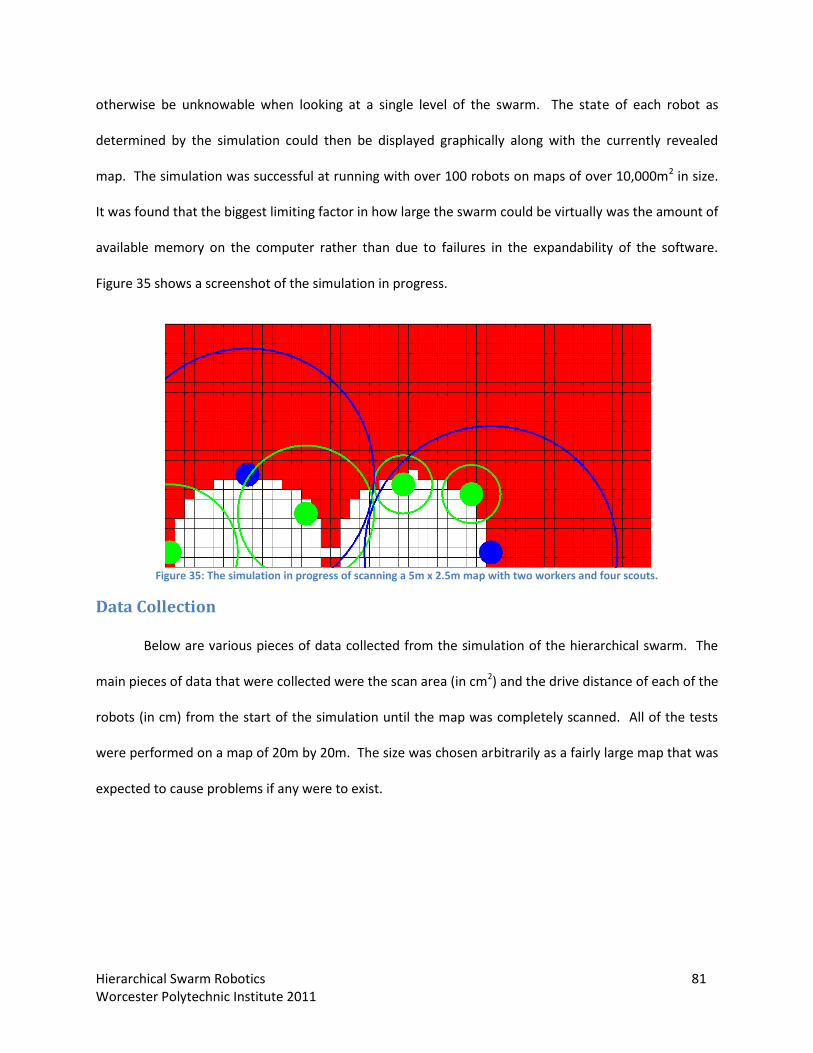
Hierarchical Swarm Robotics 81 Worcester Polytechnic Institute 2011
otherwise be unknowable when looking at a single level of the swarm. The state of each robot as
determined by the simulation could then be displayed graphically along with the currently revealed
map. The simulation was successful at running with over 100 robots on maps of over 10,000m2 in size.
It was found that the biggest limiting factor in how large the swarm could be virtually was the amount of
available memory on the computer rather than due to failures in the expandability of the software.
Figure 35 shows a screenshot of the simulation in progress.
Figure 35: The simulation in progress of scanning a 5m x 2.5m map with two workers and four scouts.
Data Collection
Below are various pieces of data collected from the simulation of the hierarchical swarm. The
main pieces of data that were collected were the scan area (in cm2) and the drive distance of each of the
robots (in cm) from the start of the simulation until the map was completely scanned. All of the tests
were performed on a map of 20m by 20m. The size was chosen arbitrarily as a fairly large map that was
expected to cause problems if any were to exist.

Hierarchical Swarm Robotics 82 Worcester Polytechnic Institute 2011
Figure 36: Average scan are of the Level 1 and Level 2 robots compared to the total number of robots.
This first graph shows the average scan area for both the level 1 and level 2 robots of the swarm
compared to the total number of robots in the swarm. Level 0 is not shown on the graph since its scan
area is simply equal to the total area of the map. The graph shows that for both the level 1 and level 2
robots, the average scan area decreases as the number of robots in the swarm increases. The level 1
robot’s are slightly more sporadic most likely caused by the large minimum bubble size. As a
consequence of the coverage algorithm, trying to fit larger bubble sizes can sometimes result in the
same area being scanned multiple times. The level 2 robots, however, can be seen to have a smooth
decay in terms of how much area each robot is scanning. The level 2 robots’ average scan area is shown
in greater detail and discussed below.
0
2000000
4000000
6000000
8000000
10000000
12000000
14000000
16000000
0 10 20 30 40 50 60 70
Ave
rage
Sca
n A
rea
(cm
2)
Number of Robots
Average Scan Area vs. Number of Total Robots
Level 1 Area Scanned
Level 2 Area Scanned

Hierarchical Swarm Robotics 83 Worcester Polytechnic Institute 2011
Figure 37: Average scan are of level 2 robots compared to the total number of robots.
The above graph shows the average scan area of the level 2 robots compared to the total
number of robots. There are 6 different series on the graph, one for each of the various number of level
1 robots used while testing. Specifically, every combination between two level 1 robots to seven level 1
robots, with two to eight level 2 robots operating per level 1 robot were tested. The collected data
shows an interesting fact, that the average scan area is actually entirely dependent on the total number
of robots, and the number of mediator robots (any robot on a level higher than the leaf node) does not
actually increase or decrease the total amount of work of the leaf node robots. That means that if a
swarm were to reach a communication or computational bottleneck, it is possible to add an additional
mediator robot at whatever level is needed without worrying about increasing the overall workload of
the swarm. Similar results were found when looking at the overall drive distance of the various robots
in the swarm.
0
500000
1000000
1500000
2000000
2500000
3000000
5 15 25 35 45 55 65
Scan
Are
a (
cm
2)
Number of Robots
Average Scan Area vs. Number of Total Robots
2 Workers: Scout Scan Area
3 Workers: Scout Scan Area
4 Workers: Scout Scan Area
5 Workers: Scout Scan Area
6 Workers: Scout Scan Area
7 Workers: Scout Scan Area

Hierarchical Swarm Robotics 84 Worcester Polytechnic Institute 2011
Figure 38: Average drive distance of Level 2 and Level 1 robots compared to the total number of robots.
Similar to the average scan area of the robots, the average drive distance also shows a general
decrease as the total number of robots increases. The red series is the average drive distance of the
Level 1 robots of the swarm. The data shows that while the drive distance goes down slightly, overall
the average drive distance of the level 1 robots does not decrease very much on a map of this size. The
reason for this is that the workers have such a large maximum bubble size that they are never utilized to
their full capacity. On a map that is 20m by 20m, since most of the work of the level 1 robots is actually
performed by the level 2 robots, their work does not increase substantially. In fact, there is almost no
increase in the number of iterations of the coverage algorithm the level 0 robot has to perform for two
level 1 robots on a 20m x 20m map instead of seven level 1 robots. However, since most of the driving
and scanning is actually performed by the level 2 robots, their drive distance can be seen to decrease
rapidly with the increase in total robots. This data closely mirrors the results seen when analyzing the
average scan area.
0
5000
10000
15000
20000
25000
30000
0 10 20 30 40 50 60 70
Ave
rage
Dri
ve D
ista
nce
(cm
)
Number of Robots
Average Drive Distance vs. Number of Total Robots
Level 1: Distance Driven
Level 2: Distance Driven

Hierarchical Swarm Robotics 85 Worcester Polytechnic Institute 2011
Results
Mechanical Results
Overall the mechanical design and implementation of the robots was a success. Throughout the
design process there were things that were done well, and things that could have been done better.
When analyzing the structural aspects of the design that could have been improved, a couple of aspects
stand out. Firstly, the amount of revisions needed to come up with the finalized design was excessive
and could have been avoided. Increased amount of peer review of each design could have reduced the
number of revisions between the initial design and the final product. The second structural design issue
was the ease of repair of other mechanical parts. The design and initial construction of the robot was
simple, however if any non-structural part broke, the design would cause the broken piece to be very
hard to reach and repair.
When analyzing the mechanical attachments to the structure of the robot that could have been
done better, one key issue stands out. The initial design of the drive shaft was thought to be sound but
instead showed flaws while testing. The initial shaft was made using cut aluminum tube in order to
mate a circular motor shaft with a square drive axel. It was thought that the tolerances provided with
cutting them by hand would be fine, but this proved incorrect after minor testing. New shafts were
designed with the testing results taken into consideration, unfortunately, due to complications with the
Rapid Prototyping Machine (RPM) they were never installed on the final version of the robots.
With these issues, there were also aspects of the mechanical design that were done very well
and resulted in successful outcomes. Structurally, the physical strength of the robot, along with its ease
of assembly was key. The interlocking acrylic pieces provided a high amount of strength, making
physically breaking the robot very difficult. Only once or twice did an acrylic piece snap due to
mishandling, and this was able to be easily fixed with glue. Since the structure was designed with
Hierarchical Swarm Robotics 86 Worcester Polytechnic Institute 2011
interlocking pieces, assembly was fairly simple, with glue being applied to slotted pieces, and being held
together for a couple minutes. In this way, an entire robot could be structurally assembled in under an
hour.
The mechanical attachments of the robot also had some well designed aspects. Specifically, the
mounting of the motors, and the encoders stood out as successful designs. The motor mount design
kept the motors well secured and left the electrical wires easily accessible. The encoders, although a
secondary design addition, were very securely mounted on the outer edge of the robot.
The casters on front and rear kept the robot balanced, while the rubber tread wheels had plenty
of friction to not slip on normal smooth surfaces. The accuracy of the robot localization, as stated
before, was only limited by the accuracy of the encoders, which in turn was limited by our budget. The
mechanical design could be changed to be better in several ways, but successfully accomplished the
goals decided on in the initial planning stages.
Electrical Results The electrical design component of this project enjoyed some success but was not without its
shortcomings. The first major setback was that the optical mouse sensors were found to be unsuitable
for odometry based navigation. The second problem encountered was the highly limited range on the
IR ‘heat’ sensors. Despite these problems, the core desired functionality still existed and the vast
majority of the electronics worked flawlessly.
The optical mouse sensors were intended to be the primary means of localization due to their
immunity to wheel slip and their high resolution. Initial testing also appeared quite promising. Once an
enclosure was built to properly hold the sensors they were very sensitive to even small movements and
could correctly be translated around a flat surface without accumulating excessive drift. The problem
occurs when a second sensor is added. An individual sensor has a nominal resolution of 2000
Hierarchical Swarm Robotics 87 Worcester Polytechnic Institute 2011
counts/inch, however this value changes drastically with respect to the height of the sensor above the
ground. If the sensor differs as much as .1mm from the ideal height, the resolution is affected largely
enough so that it is rendered useless for odometry. With a single sensor, the translation error is
somewhat manageable. Once a second sensor is added, each sensor has a slightly different resolution
and therefore accumulates a very large amount of angular drift. The reason for this is because if the
mouse sensors are placed 5cm apart, a difference in resolution of only 1% will cause the orientation of
the robot to drift by over 2 degrees for every 10cm of driving ((10*1.01 – 10*.99)/5= .04 radians= 2.3
degrees). This performance was not nearly reliable enough to allow for the usage of the sensors which
resulted in their removal from the design.
The second problem arose from difficulties in the IR heat detectors. In an effort to cut down on
cost, the IR heat detectors were built from scratch rather than using a premade solution. Unfortunately,
the custom IR detector had a range of only a few inches which does not even exceed the outer
perimeter of the robot itself. The problem appears to be that the IR LED selected for use as a stand-in
for a candle did not emit enough power to result in any reading with the sensor. Another issue was that
due to time constraints there would not be sufficient time to build the simulated candle IR beacons as
well as have a method for remotely turning them on or off. As the real focus of the project was on the
nature of a hierarchical swarm topology and not on the specifics of firefighting, it was deemed best to
drop the firefighting aspect from the design and refocus on mapping and swarm communications.
With the exception of the two problems noted above, the electrical components of the project
worked quite well. When the encoders became the primary sensor for navigation it was found that
after a robot is told to drive in a pseudo-random pattern for 100 meters, the accumulated drift is
roughly 50cm which accounts for 5mm of drift for 1 meter of driving. For conservative results this
number was rounded up to 1cm per meter of driving for use when the standard deviation of an obstacle

Hierarchical Swarm Robotics 88 Worcester Polytechnic Institute 2011
that was detected is sent to a parent. The XBee modules were also found to be highly reliable and
capable of providing a full end to end communication between modules. Another success was found in
the Sharp IR rangefinders which were found to be capable of measuring the distance to an obstacle
accurately out to 80 cm and even as close as 8 cm (smaller than the size of the physical robot). Finally,
the battery life of an individual robot is roughly 2 hours which is due in part to the highly efficient
switching regulators used as opposed to the less efficient linear regulator alternative. Another major
contributor to the battery life was the ability to completely disconnect components when they were not
in use which prevented devices like the IR rangefinders or servo turret from being a continuous drain on
the batteries. In conclusion, although the optical mouse sensors and heat detection did not perform as
needed, the more important aspects of the project such as communication and mapping did function as
good as or better than expectations.
Software Results As the bulk of the project design was in software, the results were perhaps the most telling as
far as successes and failures. Among the successes in the software design was the proven functionality
of the coverage algorithm, as well as the overall expandable design not limited to the three-tier
implementation done in this project. In contrast, some of the shortcomings of the software lie in the
organization of the probability map and related classes as well as being rather fragile.
The major victory of the software design, and perhaps the project overall, is the expandability of
the swarm with the current software implementation. While the code may appear to be implemented
specifically for the three-tier implementation, it can in fact be theoretically any number of levels deep,
with a single Queen, any levels between zero and n – 1 as Workers, and Scouts at the bottom of the
tree. This should not be misconstrued as a requirement for a balanced uniform hierarchy either. In other
words, there is no requirement that all robots of a given level need the same number of children or that
all branches must go equally deep. Due to the information hiding and selective ignorance of each level,

Hierarchical Swarm Robotics 89 Worcester Polytechnic Institute 2011
it has no knowledge other than its immediate subordinates. While this demonstrates a great amount of
flexibility, it does not serve a significant advantage with the current implementation. This does, on the
other hand, have merit if the idea of “work” is implemented as well as asynchronous assignment of work
to children. In a hypothetical task, a swarm may have to scan the surface of the earth. This rather
mighty job would likely require a swarm several levels deep, so the order in which it completes the task
is difficult to predict. What if it were imperative that the District of Columbia, Philadelphia, PA, and
Boston, MA be completed as soon as possible? With a uniform hierarchy, it is difficult to ensure this will
happen, but if a much shallower branch was deployed as a special task force, these areas could be
prioritized without sacrificing the best coverage for the bulk of the swarm. The shallower branches will
complete and report to the queen much faster than the deeper branches would be able to. This
example shows the flexibility of the design as a whole.
A small success along the lines of expandability is the potential flexibility for the platform. In
theory, this code would work just as well on any platform able to localize and run a Java application. The
swarm could consist of hovercraft, legged robots, treaded robots, etc. with no more adjustment than
physical size considerations and adjusting the heuristic for movement cost.
Another area in which the software can be considered successful is the coverage algorithm. As
stated before, the problem of coverage in a multiple agent system is an intractable problem, so finding
the optimal solution was not a reasonable goal. Instead, a greedy approach was used, making use of a
heuristic weighing the cost of moving robots versus scanning map cells. This result was not likely to be
optimal, but was clearly sufficient and completed the task reasonably without a massive computational
overhead. The approach always attempted to place all robots over keeping a certain size scan radius. For
higher levels, this makes complete sense, as it doesn’t make sense to discard a level 1 robot for an
iteration when it could reduce their bubble size. Since a scanned area could very easily take a long time,
it is not very good utilization to have half the swarm sit idle. Approaching the leaf nodes however, this is

Hierarchical Swarm Robotics 90 Worcester Polytechnic Institute 2011
not always the best choice. For instance, it is a little more efficient for the Scouts in the three-tier swarm
to be removed and allow the others to have larger scan bubbles than to maximize the number of robots
placed upon reaching a minimum scan radius. While not impossible to change the way the coverage
algorithm chooses child locations and scan radii, it violates the hidden information somewhat, since it
knows that its children are better placed with larger bubbles than larger quantity. This infraction is not
severe though, as it doesn’t know this would be because the Scouts have no children, merely that it is
advantageous for some reason. After analyzing the benefits and shortcomings of both, it was decided
simply to use the original priority of placing robots over maximizing the bubble sizes. This was for two
reasons; the software remains significantly more generic by having a uniform selection across levels, and
that the benefit on the lowest level was not significant enough to be worth the added complexity.
As an extension of the coverage algorithm’s success, the robots were placed and given move
orders in such a way that the physical robots could move around safely and without worry of colliding
with one another. This was not all handled directly by the coverage algorithm, but by the union of
various methods for handling robot placement and path planning. This created a good system to work
with the placements chosen by the coverage algorithm. The simulation was paramount in finding and
debugging this sort of problem before testing things on the physical swarm. One of the tools which
helped achieve this was the “wave generator,” which detected intersections between child paths (or
paths close enough to be problematic) and would send children in waves to guarantee avoiding a
collision. Another tool was the “move idle robots” method which determines the best place to move
robots not placed by the coverage algorithm, but are in the way of other robots scanning. Although both
of these appear to be benign problems, ignoring them would have been serious mistake.
A very important success in this project that was briefly mentioned above is the simulation. In
the real world, robot localization is at best, imperfect, as is the case with any sensor data. Regardless of
how accurate or precise the sensors are (especially using odometry), or how good of a model the

Hierarchical Swarm Robotics 91 Worcester Polytechnic Institute 2011
Kalman filter has, there will be error. Like so many high-school physics problems, the simulation can
operate in a theoretically perfect and simplified environment without error. It is worthy of noting,
however, that the code running on the simulated robots is exactly identical to that of the physical
implementation. The only thing that makes those robots simulated is their kinematics being updated
without the need to drive, and the communication being handled without hardware. Since the
simulation is such an accurate representation of the actual swarm behavior, it was used for most of the
data collection. It could properly test many metrics of swarm performance in a tiny fraction of the time
it would take to observe the physical swarm.
The software design had its shortcomings as well. An increasingly obvious problem with the
software design was that of the probability map (ProbMap) class. This served as the hub for all data
regarding the map, and also nearly every interface and function to it. While the class quickly became a
bit unwieldy, it couldn’t be considered a ‘failing’ early on. The final nail in the coffin for the class was the
failure to properly use or distinguish between internal units (using the map index) and external units
(using centimeters). The class’s abundant interfaces often use index references to obtain and set cell
information, however it has become clear that all public methods of the map should have been made
using centimeters, and all private methods can be allowed to use internal units where appropriate. A
common error while writing code in other sections of the program was to accidentally use internal units
where it should have been external units, or visa-versa. Despite the commonality of these errors, they
were not always immediately evident, wasting valuable time. This became extremely problematic as the
class added more and more functionality. Needless to say, many lessons were learned while working
with this class, and those mistakes would not be made again.
A less severe issue was the improper organization and interdependencies in some of the more
complicated sections of the code. Using the term “spaghetti code” might be a bit harsh and inaccurate,
as the program flow was not unstructured or particularly confusing, but the problem is still worthy of
Hierarchical Swarm Robotics 92 Worcester Polytechnic Institute 2011
noting. For instance, the moveIdleRobots method has direct dependencies on data configured by the
coverage algorithm while they should be completely separate. This brings attention to the real
underlying problems, which are the lack of defensive programming and the fragility of the code as a
whole. The flow of the system was designed very well assuming no failures were encountered at any
point. Unfortunately, if an error did occur, (Java exception, missed packet, etc.) there was no way to
recover from it, and the entire swarm would halt and either crash or hang indefinitely. There were some
proposed ideas for making the code less fragile, however none of them were simple enough to be
completed in a reasonable timeframe, often calling for a complete system overhaul.
Discussion The goal of this project was to create a proof of concept hierarchical swarm. This was
successfully achieved by creating a three tiered swarm consisting of one level 0, two level 1’s, and four
level 2’s. The result was a swarm that was capable of autonomously mapping an unknown area
approximately 2.5m by 2.5m. This swarm was considerably different than other attempts at swarm
mapping solutions due to the hierarchical structure. Many other solutions utilize the interconnected
topology which can result in a significant increase in the number of communication lines present
between all the robots. The swarm was then expanded by using a simulation of the robots and their
communication structure in order to run it on a greater number of robots. The simulation has
successfully been run with over 110 robots until the computation limits of attempting to run what is
supposed to be an entirely distributed system on a single computer were reached. The project was also
successful in creating an abstract coverage algorithm capable of placing any number of robots on a map
such that they can all scan as much area as possible.
Originally, the goal of the project was to create a hierarchical swarm designed to find and
extinguish fires within a large unknown environment (specifically the gymnasium). This task however
was soon determined to be far beyond the budget or scope of the project. Therefore, the original

Hierarchical Swarm Robotics 93 Worcester Polytechnic Institute 2011
objective was relaxed to focus on mapping a smaller area in order to prove the core hierarchical
concept. Additionally, due to time limits the mid level robots were never constructed and instead were
made entirely virtual. While they do run the same code as the actual robots (as discussed in the
simulation section), they were also supposed to be driving with the scouts in the unknown map. Instead
they were left as programmed entities without any physical bodies. The children in the map will act as if
the workers are in the map and will route around them when going from place to place.
Future Work The following sections outline a few features that would have been desirable to implement
however were left out due to time constraints.
Node Failure Detection One feature that would be a nice addition is node failure detection, or the ability to gracefully
recover from any node going offline in the swarm. This is made particularly difficult due to the abstract
nature of the swarm and the fact that, for example, if a Level 1 node were to die, all of the level 2 nodes
would have to find a way to become re-distributed throughout the swarm, which may potentially break
previously set communication rules. While there have been some ideas for implementation, after much
deliberation there remain two central problems. First, how does a node in the swarm detect that
another node has failed, and how does a node recover from such a failure, with the best case being that
no communication protocols are broken.
It was determined that that best way to check for a node failing in the swarm was to monitor
communications. One way to do this was the idea of a “heartbeat” thread that would reset a counter
each time a node receives a message from its parent or the other way around. If too much time passed
the robots would check to see if the corresponding node was still operational by sending some form of
Hierarchical Swarm Robotics 94 Worcester Polytechnic Institute 2011
communication and then waiting for a reply. If too much time elapsed, then the sending node would
assume the other had died and take steps to correct the issue.
No ways of re-distributing the swarm were found that did not involve breaking the strict
communication rules developed earlier. The only way of moving around resources was to have the
children of the parent communicate to the other robots in the same level as the parent and be assigned
accordingly. The process is that the children would communicate to the next level up that they were
free and could be re-assigned to anyone. Another complex issue was that even once children were
reassigned to a new parent, the children would be outside their new parent’s bubble. Therefore, the
parent would not have a valid way of routing the orphaned robots from their current location to
somewhere inside the bubble.
Emergency Stop / Other Safeties In addition to the ability for the swarm to adapt gracefully if a node were to die, the swarm also
currently lacks many general safety features. There are a variety of these in terms of both software and
hardware implementations that would be useful additions.
The first safety feature would be an emergency stop command that could be sent to any or all
nodes in the swarm in order to cause them to immediately stop whatever command is executing and
wait for further instructions. This would be useful in the event that the queen or human operator who
noticed imminent danger could stop the swarm from progressing, and specifically be able to resume the
swarm once the danger had passed or things were adjusted. Currently the swarm has the ability to be
killed entirely, which will perform the stopping ability, but then has no way of resuming later.
Hardware-wise, there is also no protection for the swarm in case a node was to drive off an edge and fall
to harm. The addition of sensors to detect such falls or other dangerous obstacles would be a nice
addition; however it is hard to cover all the possibilities since the physical hazards are rather
Hierarchical Swarm Robotics 95 Worcester Polytechnic Institute 2011
implementation specific. In particular, the board developed for this project does have the ability to use
bump sensors if they were added to the robot body in case the robot were to hit an obstacle.
Unfortunately due to time constraints, the bump sensors were never added to the robots causing them
to be unable to detect a collision.
SLAM and the UKF One of the limiting factors noted throughout the project is the lack of scalability involved with
odometry. Odometry can be improved by using better and better sensors however it is fundamentally
flawed in the sense that it is entirely open loop and is not able to correct itself as it drifts further and
further from the correct pose. There are two proposed methods of fixing this problem. The first and
easiest is to simply incorporate a sensor capable of measuring absolute location such as GPS. The
problem with simply relying on GPS location is that there will likely be a large amount of noise in the
signal causing the robot to appear as if it is rapidly ‘jittering’ around a given point. This can be corrected
through an averaging filter or more intelligently through a Kalman filter. Even this method however has
its problems. Mainly the issue is that for indoor localization, GPS will likely be unavailable. Other
localization techniques that do work indoors are either not accurate enough or are simply too expensive
to be practical. Although it is outside the scope of this project to actually implement, it is worth
discussing how localization could theoretically be improved.
The solution to this problem is to use simultaneous localization and mapping (SLAM). SLAM is
based on the principal that as a map is constructed a robot should be able to determine its own position
relative to that map. This process lends itself well to be implemented with a Kalman filter because the
prediction equation can be fulfilled with the robot’s odometry data, and the update equation can
correct the odometry data using the newly gathered map data. This process however is non-linear due
to the use of sine and cosine when calculating the displacement of a robot at a given heading.
Therefore, SLAM is typically done with an extended Kalman filter. The extended Kalman filter (EKF)

Hierarchical Swarm Robotics 96 Worcester Polytechnic Institute 2011
works similarly to a standard Kalman filter, however it linearizes the equations using a first order
approximation typically done with Jacobian matrices [20]. The unscented Kalman filter (UKF) further
improves upon this by using a process known as the unscented transform to achieve greater than first
order approximations without having to calculate the Jacobian [20].
The first step in any SLAM algorithm is to be able to identify features or landmarks which could
be observed and re-identified at a later time. One type of landmark that works well is a wall. For the
sake of discussion assume that a robot has a sensor which can detect the range and azimuth to an object
and is capable of calculating the sample point’s x, y location in the Cartesian plane. A wall would be
observed by the robot as a set of blocked areas which happen to fall on a straight line. The landmark
being composed of multiple sample points helps reduce the effects of noise and makes the identification
more reliable. The next question is now how to determine which sample points to associate with a wall
and which should not be. The idea of a linear best fit line is a good start, but this approach would be
defeated if two separate walls can be observed such as the intersection at a corner. A better approach
is to use the random sampling and consensus algorithm (RANSAC). This algorithm works by first
selecting a point at random out of all sample points. Then, a small number of nearby points are selected
and a linear regression is applied to this small sample. From there, the linear fit is checked against all
sample points and if enough of the sample points are on or near the line then the line equation is
assumed to correspond to a wall. This process is then repeated until either every sample point is on or
near a line, or until the process exceeds a given number of iterations. The algorithm is tuned by varying
parameters such as the number of iterations to run, how close a point must be to a line to be considered
on the line, or the number of points which must lie on the line to consider it a wall. Despite the random
nature of the selection, the algorithm can provide good performance. The major benefit is that there is
no limit to the number of lines which can be extracted from a given set of data. It is also very good at
ignoring outliers or even small gaps in a wall [21].

Hierarchical Swarm Robotics 97 Worcester Polytechnic Institute 2011
Once a wall has been identified, it is convenient to represent the line as if it were a single point,
both for remembering the location of the landmark as well as comparing future sightings to see if the
landmark is the same. One method for doing this is to draw a line from the origin (or any other agreed
upon arbitrary point) to the wall such that the line drawn intersects the wall at a right angle. The point
of intersection is the point which the wall is ‘condensed’ into. At this point, the algorithm has found all
walls and is now storing each wall as a single point. When future scans observe walls, a simple heuristic
to determine if a wall has been seen before is to simply compare the expected location of any wall with
all observed walls and assume whichever observed point is nearest to the expected location is the true
location of the wall. This is also known as the nearest neighbor approach [21].
Now the robot has a map of all known landmark locations (walls) as well as the new positions of
newly observed walls (many of which are simply the old walls re-observed). Using this information
allows the robot to compare where it believes it is located against known reference points in the map to
correct for errors in the belief state. This is a perfect job for the UKF. The full steps for the UKF are
listed below [22].
Predict:
1. xak-1|k-1 = [xk-1|k-1
T E[wk]T]T
Augment the state matrix x with the expected mean value for the noise wk (likely zero)
2. Pak-1|k-1 = [Pk-1|k-1 0; 0 Qk]
Augment the covariance matrix P with the covariance matrix Q which is a covariance matrix of
the state matrix x
3. χ0k-1|k-1 = xa
k-1|k-1
χ ik-1|k-1 = xa
k-1|k-1 + (sqrt((L + λ)Pak-1|k-1))i i= 1..L
χ ik-1|k-1 = xa
k-1|k-1 - (sqrt((L + λ)Pak-1|k-1))I - L i= L+1 .. 2L

Hierarchical Swarm Robotics 98 Worcester Polytechnic Institute 2011
Derive 2L + 1 sigma points from the augmented state where L is the dimension of the
augmented state. (sqrt((L + λ)Pak-1|k-1))i is the matrix square root of the ith column of (L + λ)Pa
k-
1|k-1 and λ= α2(L+κ) – L where α and κ are scaling parameters typically set to 10-3 and 0
respectively.
4. χ ik|k-1 = f(χ i
k-1|k-1, uk-1) I = 0..2L
Perform the nonlinear prediction equation where u is the input vector if it exists.
5. xk|k-1 = Σi= 0..2L Wsi χ i
k|k-1
Pk|k-1 = Σi= 0..2L Wci [χ i
k|k-1 – xk|k-1] [χ i
k|k-1 – xk|k-1]T
Ws0 = λ/(L + λ)
Wc0 = λ/(L + λ) + (1 – α2 + β) (β is set to 2 for Gaussian noise, α is same as before)
Wsi = Wc
i = 1/(2(L+λ))
Recombine sigma points with given calculated weights.
Update
1. xak|k-1 = [xk|k-1
T E[wk]T]T
Pak|k-1 = [Pk|k-1 0; 0 Rk] Where Rk is the noise covariance
2. χ 0k|k-1 = xa
k|k-1
χ ik|k-1 = xa
k|k-1 + (sqrt((L + λ)Pak|k-1))i i= 1..L
χ ik|k-1 = xa
k|k-1 - (sqrt((L + λ)Pak|k-1))I - L i= L+1 .. 2L
3. yik = h(χ i
k|k-1) I = 0..2L
Perform nonlinear update measurement equation.
4. z’k = Σi= 0..2L Wsi yk
i
5. Pkk = Σi= 0..2L Wci [yi
k – z’k] [yik– z’k]
T
6. Pxkk = Σi= 0..2L Wci [Xi
k|k-1 – xk|k-1] [yik– z’k]
T

Hierarchical Swarm Robotics 99 Worcester Polytechnic Institute 2011
7. Kk = Pxkk Pkk-1
Compute Kalman gain
8. xk|k = xk|k-1 + Kk(zk – z’k)
Update the state with measurement vector zk
9. Pk|k = Pk|k-1 – KkPkkKkT
Update the covariance matrix
As the previous equations state, the UKF constantly predicts the next state (in this case with odometry
data) and then corrects the state with measured data (in this case with the map landmarks). The UKF
performs well even with highly nonlinear equations and requires no Jacobian derivative calculations.
The only two equations which are required are the prediction equation f(x):
[x y θ]T = [x+d cos(θ) y+d sin(θ) θ+φ]T
Where d is the forward distance driven and φ is the change in orientation.
The second equation needed is the update equation h(x):
[sqrt((x – xl)2 + (y – yL)
2) atan2(y – yl, x – xL) .. ]T
The first entry in the matrix is the range to a landmark and the second is the bearing to it. xL, yL
is a landmark location and the measurement matrix contains one range bearing pair for each
landmark observed.
Although due to its computational complexity and complicated mathematics,
implementing this filter was deemed outside the project scope. However, such a filter would
greatly help improve the expandability of the swarm as it would allow for the mapping of larger
areas without the limitations imposed by odometry.

Hierarchical Swarm Robotics 100 Worcester Polytechnic Institute 2011
Social Implications Another important consideration is where this project could lead to in terms of real-world
applications. This project aimed to develop a new highly scalable swarm architecture capable of being
used in a variety of ways. The swarm can be highly heterogeneous which allows the swarm to be used
for tasks such as firefighting, search and rescue, and environmental cleanup. For firefighting, the swarm
could be divided such that one level searches for fires while another level is tasked with putting the fires
out. Search and rescue applications could employ a mixture of ground and aerial robots. The aerial
robots could focus on surveying an area while the ground units could focus on rescuing the survivors.
For an environmental cleanup swarm, one level could contain oil spills while another separates and
removes oil from already contaminated water. As all these examples demonstrate, the hierarchical
ideas proposed in this paper are intended to be more general rather than application specific. Although
traditional swarm topologies are still applicable to these problems, the hierarchical topology proposed
aims to greatly improve the scalability of a swarm to much greater levels than would be possible with a
swarm running an interconnected or ring topology.
This project also explored some of the aspects required to implement a swarm as an actual
product. The robots were made mostly out of cheap acrylic to allow for cheap manufacturing and also
were made into a rounded shape to reduce the risk of injury during handling. ROHS components were
used wherever possible to promote ecological construction. In addition to ROHS, additional standards
on the mechanical and electrical design were used whenever necessary. Such standards included design
considerations when making the custom circuit board as well as the robot chassis.
All data and results in this project are portrayed in an ethical manner. The meaning behind this
is that none of the data has been intentionally misrepresented in order to portray a different point than
what would normally be inferred from the data. The tests were complete and well documented. All
claims as to the ability of our swarm mentioned in the paper or any other presentation of the above and

Hierarchical Swarm Robotics 101 Worcester Polytechnic Institute 2011
below work directly stem from our hypothesis as supported by the data. This project lies on the
precipice of human knowledge within the confines of combining hierarchies into swarm system. The
introduction of this new knowledge to the swarm and robotic communities indicates that learning is in
fact never finished and continues for a lifetime.
Conclusion In conclusion, the goal of this project was to create a proof of concept hierarchical swarm. This
goal was successfully accomplished by creating a three tier swarm capable of autonomously mapping an
unknown area. While this implementation used four physical robots and three virtual robots, it was
successfully virtualized using up to 111 virtual robots to scan a significantly larger unknown space.
While the project did not compare the viability of a hierarchical swarm when compared to already
existing swarm topologies, it did show that a hierarchical swarm can in fact be used to solve problems
well suited for distributed robotic systems. The intent of this paper is to fill a void found while
researching hierarchical information structures in robotics as well as multi-robot sensor based area
coverage. With the success of this project, future work can be now performed in order to compare
hierarchical topologies to other, better established, forms of swarms. Specifically, research could be
conducted to show the ability of a hierarchical topology to solve a problem when pit against an
interconnected or ring topology.
Hierarchical Swarm Robotics 102 Worcester Polytechnic Institute 2011
Bibliography 1. Dorigo, Marco, Birattari, Mauro and Stützle, Thomas. Ant Colony Optimization. s.l. : IEEE
Computational Intelligence Magazine, 2006.
2. Akbari, Reza, Mohammadi, Alireza and Ziarati, Koorush. A Powerful Bee Swarm Optimization
Algorithm. s.l. : IEEE, 2009.
3. Ederhart, Russell and Kennedy, James. A New Optimizer Using Particle Swarm Theory. s.l. : Sixth
International Symposium on Macro Machine and Human Science, 1995.
4. Liu, Changlei and Cao, Guohong. Spatial-Temporal Coverage Optimization in Wireless Sensor
Networks. s.l. : IEEE Transactions on Mobile Computing, 2011.
5. González, Enrique, et al. BSA: A Complete Coverage Algorithm. s.l. : International Conference on
Robotics and Automation, 2005.
6. Easton, Kjerstin and Burdick, Joel. A Coverage Algorithm for Mutli-Robot Boundary Inspection. s.l. :
Californ Institute of Technology.
7. Schor, D., Kinsner, W. and Anderson, J. A Study of Optimal Topologies in Swarm Intelligence.
8. Chen, Hanning, et al. Hierarchical Swarm Model: A New Approach to Optimization. s.l. : Hindawi
Publishing Corporation, 2010.
9. Jones, Frank and Soule, Terence. Dynamic Particle Swarm Optimization via Ring Topologies. s.l. :
GECCO, 2009.
10. Mohan, Yogeswaran and Ponnambalam, S. G. An Extensive Review of Research in Swarm Robotics.
Selangor : IEEE, 2009.
11. Bonabeau, Eric, Dorigo, Marco and Theraulaz, Guy. From Natural to Artificial Swarm Intelligence.
s.l. : Oxford University Press, 1999.
12. Holland, Owen and Melhuish, Chris. Stigmergy, Self-Organization, and Sorting in Collective Robots.
s.l. : MIT, 1999.
13. Matsushita, Haruna and Nishio, Yoshifumi. Network-Structured Particle Swarm Optimizer with
Small-World Topology. 2009.
14. Surve, Sunil, Dr. Singh, N. M. and Dr. Lande, B. K. CPPA: A Fast Coverage Algorithm. 2007.
15. Wang, Xudong and Syrmos, Vassilis L. Coverage Path Planning for Multiple Robotic Agent-Based
Inspection of an Unknown 2D Environment. 2009.
16. Engineer's Handbook. Engineer's Handbook. [Online] 2006. [Cited: April 26, 2011.]
http://www.engineershandbook.com.
Hierarchical Swarm Robotics 103 Worcester Polytechnic Institute 2011
17. AutoWare. Ackerman Steering and Racing Circle (oval) Tracks. [Online] 2009. [Cited: April 26, 2011.]
http://www.auto-ware.com/setup/ack_rac.htm.
18. Dijkstra, E. W. A Note on Two Problems in Connexion with Graphs. s.l. : Numerische Mathematlk,
1959.
19. McNeill, James. Raytracing on a Grid. Playtechs: Programming for Fun. [Online] Blogspot, March 26,
2007. [Cited: April 27, 2011.] http://playtechs.blogspot.com/2007/03/raytracing-on-grid.html.
20. Julier, Simon J. and Uhlmann, Jeffrey K. A New Extension of the Kalman Filter to Nonlinear Systems.
Oxford : The University of Oxford, 1997.
21. Riisgaard, Søren and Blas, Morten Rufus. SLAM for Dummies: A Tutorial Approach to Simultaneous
Localization and Mapping . Boston : MIT, 2004.
22. A.Wan, Eric, Merwe, Rudolph van der and Nelson, Alex T. Dual Estimation and the Unscented
Transformation. Portland : Oregon Graduate Institute of Science & Technology, 2000.


