Download - High-resolution atmospheric inversion of urban CO2 ... · Gurney 5,Jianhua Huang ,Darragh O’Keefe5, Yang Song5,Anna Karion6,Tomohiro Oda7,8,Risa Patarasuk5 ... tions,Htheinﬂuencefunctions,andRandB

Journal of Geophysical Research: Atmospheres

High-resolution atmospheric inversion of urban CO2 emissionsduring the dormant season of the IndianapolisFlux Experiment (INFLUX)

Thomas Lauvaux1,2, Natasha L. Miles1, Aijun Deng1, Scott J. Richardson1, Maria O. Cambaliza3,4,Kenneth J. Davis1, Brian Gaudet1, Kevin R. Gurney5, Jianhua Huang5, Darragh O’Keefe5,Yang Song5, Anna Karion6, Tomohiro Oda7,8, Risa Patarasuk5, Igor Razlivanov5, Daniel Sarmiento1,Paul Shepson9, Colm Sweeney6, Jocelyn Turnbull9,10,11, and Kai Wu1

1Department of Meteorology, Pennsylvania State University, University Park, Pennsylvania, USA, 2NASA Jet PropulsionLaboratory, Pasadena, California, USA, 3Department of Physics, Ateneo de Manila University, Quezon City, Philippines,4Manila Observatory, Ateneo de Manila Campus, Quezon City, Philippines, 5School of Life Sciences, Arizona StateUniversity, Tempe, Arizona, USA, 6CIRES, University of Colorado Boulder, Boulder, Colorado, USA, 7Global Modeling andAssimilation Office, NASA Goddard Space Flight Center, Greenbelt, Maryland, USA, 8Goddard Earth Sciences Technologiesand Research, Universities Space Research Association, Columbia, Maryland, USA, 9Department of Chemistry, PurdueUniversity, West Lafayette, Indiana, USA, 10NOAA Earth System Research Laboratory, Boulder, Colorado, USA, 11NationalIsotope Centre, GNS Science, Lower Hutt, New Zealand

Abstract Based on a uniquely dense network of surface towers measuring continuously theatmospheric concentrations of greenhouse gases (GHGs), we developed the first comprehensive monitoringsystems of CO2 emissions at high resolution over the city of Indianapolis. The urban inversion evaluatedover the 2012–2013 dormant season showed a statistically significant increase of about 20% (from 4.5to 5.7 MtC ± 0.23 MtC) compared to the Hestia CO2 emission estimate, a state-of-the-art building-levelemission product. Spatial structures in prior emission errors, mostly undetermined, appeared to affectthe spatial pattern in the inverse solution and the total carbon budget over the entire area by up to 15%,while the inverse solution remains fairly insensitive to the CO2 boundary inflow and to the different prioremissions (i.e., ODIAC). Preceding the surface emission optimization, we improved the atmosphericsimulations using a meteorological data assimilation system also informing our Bayesian inversion systemthrough updated observations error variances. Finally, we estimated the uncertainties associated withundetermined parameters using an ensemble of inversions. The total CO2 emissions based on the ensemblemean and quartiles (5.26–5.91 MtC) were statistically different compared to the prior total emissions(4.1 to 4.5 MtC). Considering the relatively small sensitivity to the different parameters, we conclude thatatmospheric inversions are potentially able to constrain the carbon budget of the city, assuming sufficientdata to measure the inflow of GHG over the city, but additional information on prior emission errorstructures are required to determine the spatial structures of urban emissions at high resolution.

1. Introduction

The increase in the atmospheric concentration of carbon dioxide (CO2) reached the fastest decadal rate overthe period 2002–2011 with 2 ± 0.1 ppm/yr. Consequently, CO2 remains the largest single contributor to theincrease in the anthropogenic radiative forcing [Intergovernmental Panel on Climate Change, 2014], with 80%of the emissions originating from fossil fuel combustion and industrial processes. Quantification of anthro-pogenic CO2 emissions is typically accomplished via bottom-up accounting or inventory methods at global[e.g., Marland et al., 1985; Andres et al., 1996, 2012; Asefi-Najafabady et al., 2014] and regional scales [Gurneyet al., 2009, 2012]. These inventories remain affected by large uncertainties [Andres et al., 2014] which increasesat higher spatial and temporal resolutions [e.g., Turnbull et al., 2011]. As legislation to regulate greenhousegas (GHG) emissions becomes increasingly likely, independent verification of inventory-based anthropogenicemissions becomes an emerging need [NRC, 2010].

Urban CO2 emissions represent about 70% of the global emissions and will likely increase as large metropoli-tan areas are projected to grow twice as fast as the world population in the coming 15 years [United Nations

RESEARCH ARTICLE10.1002/2015JD024473

Key Points:• High resolution bottom-up and

top-down fossil fuel emissions agreewithin 20% at the city scale

• Inverse urban emissions and GHGboundary inflow are well constrainedby dense tower observation network

• Undefined error structures in prioremissions impact significantly thesource attribution capability athigh resolution

Correspondence to:T. Lauvaux,[email protected]

Citation:Lauvaux T., et al. (2016), High-resolutionatmospheric inversion of urban CO2emissions during the dormant seasonof the Indianapolis Flux Experiment(INFLUX), J. Geophys. Res. Atmos.,121, doi:10.1002/2015JD024473.

Received 9 NOV 2015

Accepted 27 MAR 2016

Accepted article online 7 APR 2016

©2016. American Geophysical Union.All Rights Reserved.

LAUVAUX ET AL. URBAN INVERSION 1

http://publications.agu.org/journals/

http://onlinelibrary.wiley.com/journal/10.1002/(ISSN)2169-8996

http://dx.doi.org/10.1002/2015JD024473

Journal of Geophysical Research: Atmospheres 10.1002/2015JD024473

Department of Economic and Social Affairs Population Division, 2014]. Monitoring urban emissions usingindependent approaches is therefore a critical need for current and future regulation policies with atmo-spheric inversion techniques being a potential candidate to provide a robust and complementary approachto current reporting activities [Nisbet and Weiss, 2010]. However, a better understanding of the underlyinghuman activities remains critical for policy decisions and mitigation strategies [Hutyra et al., 2014], whichimplies the use of process-oriented systems, highly resolved in both space and time [Gurney et al., 2012].Current atmospheric inversion systems remain too coarse spatially and are limited to constraining the emis-sions rather than the underlying processes. Therefore, higher resolution inverse systems are needed to betterunderstand and quantify the emissions by sector (e.g., manufacturing sources, power generation sources, andmobile sources) in support of future policies.

This lack of well-established methods for quantifying spatially and temporally resolved GHG emissions appliesto urban areas. Recent studies have provided high-resolution emission products separated by sector [Gurneyet al., 2012] but are difficult to assemble and very likely prone to systematic errors [Gurney, 2014]. Atmosphericmethods offer a unique angle on urban emissions by capturing the accumulated atmospheric signals emittedfrom all sectors of activity [Turnbull et al., 2011]. But these methods are also limited by various sources of errors,mostly due to the atmospheric transport models [Gerbig et al., 2003; Diaz-Isaac et al., 2014] and the incorrectcharacterization of prior flux errors [Koohkan and Bocquet, 2012], as well as by the number of atmospheric mea-surements available over the region of interests. At moderate resolutions (10–40 km), atmospheric inversionsusing regional atmospheric transport models [Lauvaux et al., 2012; Schuh et al., 2013] have the potential toprovide spatially and temporally resolved GHG surface fluxes [Ogle et al., 2015]. At higher resolutions, severalstudies have shown the potential of atmospheric systems to detect emissions [McKain et al., 2012; Kort et al.,2012; Bréon et al., 2015].

The inversion of large point sources and well-defined emitting areas are particularly sensitive to the transportmodel and the representation of plume structures over flat or complex terrain, especially for observationswithin the urban domain [Bréon et al., 2015]. Large spatial and temporal gradients in urban emissions generatelarge gradients in atmospheric mixing ratios. Therefore, the development of accurate atmospheric modelingsystems able to simulate these gradients is a prerequisite to the detection and quantification of emissionsover highly contrasted urban environment. High-density observations combined with high-resolution atmo-spheric modeling have the potential to yield such resolution over small domains. At the mechanistic level, pro-cesses from specific sectors of the economy shape the spatial pattern of GHG emissions across urban centers.But atmospheric inversions have not yet been used to separate the contributions from individual sectors ofthe economy [Djuricin et al., 2012] or to separate biogenic and anthropogenic sources [Djuricin et al., 2010].Expanding the atmospheric inversion systems to include multiple trace gases, including isotopic tracers suchas 14CO2 [e.g., Kuc, 1986; Newman et al., 2008], offers the capability to measure the fraction of the signalsrelated to fossil fuel consumption and perhaps sectoral emissions. However, discrete isotopic measurementsand the lack of proper characterization of background conditions [Turnbull et al., 2015; Vardag et al., 2015] limitthe use of isotopic tracers to quantify the fluxes from highly managed vegetated areas. In order to build a firstcomprehensive atmospheric system at the urban scale, the dormant season simplifies the inverse problemwith decreased biogenic signals, contributing to only 5% of the total city plume over Indianapolis [Turnbullet al., 2015].

The Indianapolis Flux Experiment (INFLUX) is exploring the technical limits of atmospheric methods forinferring highly resolved anthropogenic GHG emissions estimates. Here we present the first atmosphericinversion system producing high-resolution GHG emissions of CO2 at the urban scale, assimilating bothatmospheric mixing ratios of greenhouse gases and meteorological measurements. The inverse modelingsystem is able to derive spatially and temporally resolved urban CO2 emissions within a large urban area,starting with a high-resolution emission product, Hestia [Gurney et al., 2012]. First, we developed an atmo-spheric four-dimensional data assimilation (FDDA) modeling system at 1 km spatial resolution assimilat-ing continuously meteorological measurements to improve the representation of the local atmosphericdynamics. Transport errors associated with the atmospheric modeling system are then quantified as a func-tion of the accuracy of different meteorological variables. Second, we demonstrate the current inversionsystem ability to monitor GHG emissions using a high-density spatially distributed atmospheric observingnetwork of instrumented towers, using two existing high-resolution CO2 emissions products. Finally, we con-struct an ensemble of inverse solutions to represent additional sources of errors in the current inversionsystem and quantify the uncertainties associated with parameters in the system.



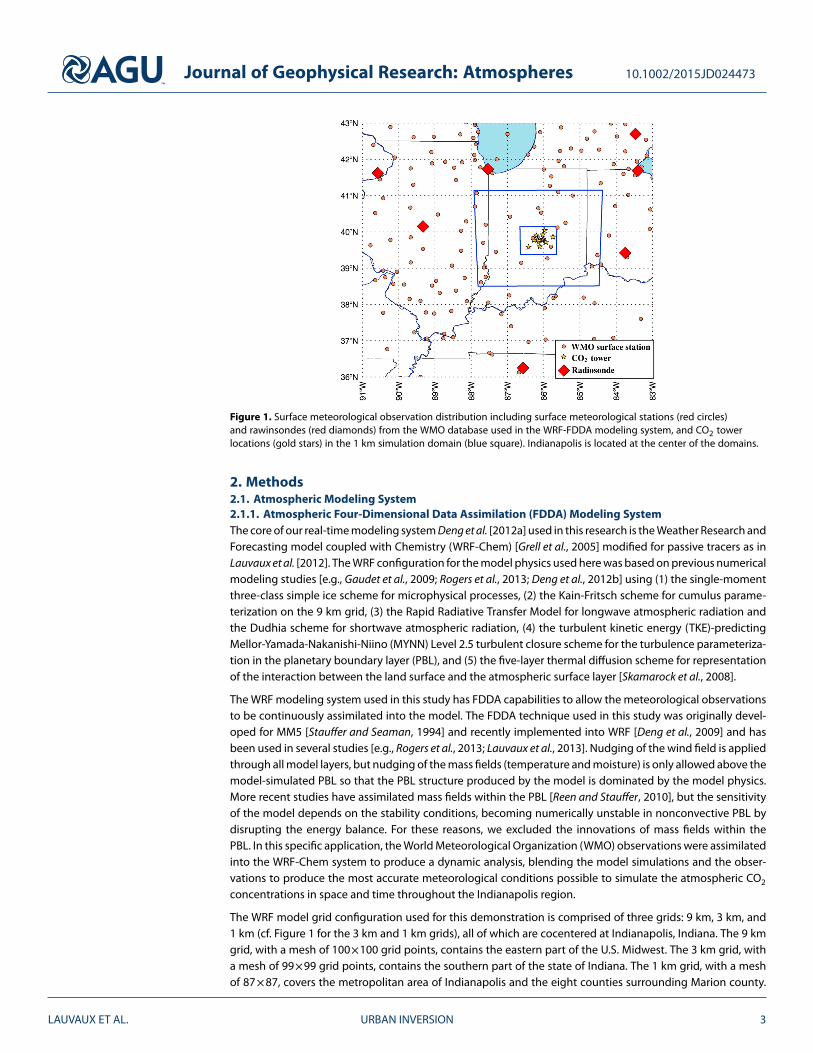
Figure 1. Surface meteorological observation distribution including surface meteorological stations (red circles)and rawinsondes (red diamonds) from the WMO database used in the WRF-FDDA modeling system, and CO2 towerlocations (gold stars) in the 1 km simulation domain (blue square). Indianapolis is located at the center of the domains.

2. Methods2.1. Atmospheric Modeling System2.1.1. Atmospheric Four-Dimensional Data Assimilation (FDDA) Modeling SystemThe core of our real-time modeling system Deng et al. [2012a] used in this research is the Weather Research andForecasting model coupled with Chemistry (WRF-Chem) [Grell et al., 2005] modified for passive tracers as inLauvaux et al. [2012]. The WRF configuration for the model physics used here was based on previous numericalmodeling studies [e.g., Gaudet et al., 2009; Rogers et al., 2013; Deng et al., 2012b] using (1) the single-momentthree-class simple ice scheme for microphysical processes, (2) the Kain-Fritsch scheme for cumulus parame-terization on the 9 km grid, (3) the Rapid Radiative Transfer Model for longwave atmospheric radiation andthe Dudhia scheme for shortwave atmospheric radiation, (4) the turbulent kinetic energy (TKE)-predictingMellor-Yamada-Nakanishi-Niino (MYNN) Level 2.5 turbulent closure scheme for the turbulence parameteriza-tion in the planetary boundary layer (PBL), and (5) the five-layer thermal diffusion scheme for representationof the interaction between the land surface and the atmospheric surface layer [Skamarock et al., 2008].

The WRF modeling system used in this study has FDDA capabilities to allow the meteorological observationsto be continuously assimilated into the model. The FDDA technique used in this study was originally devel-oped for MM5 [Stauffer and Seaman, 1994] and recently implemented into WRF [Deng et al., 2009] and hasbeen used in several studies [e.g., Rogers et al., 2013; Lauvaux et al., 2013]. Nudging of the wind field is appliedthrough all model layers, but nudging of the mass fields (temperature and moisture) is only allowed above themodel-simulated PBL so that the PBL structure produced by the model is dominated by the model physics.More recent studies have assimilated mass fields within the PBL [Reen and Stauffer, 2010], but the sensitivityof the model depends on the stability conditions, becoming numerically unstable in nonconvective PBL bydisrupting the energy balance. For these reasons, we excluded the innovations of mass fields within thePBL. In this specific application, the World Meteorological Organization (WMO) observations were assimilatedinto the WRF-Chem system to produce a dynamic analysis, blending the model simulations and the obser-vations to produce the most accurate meteorological conditions possible to simulate the atmospheric CO2

concentrations in space and time throughout the Indianapolis region.

The WRF model grid configuration used for this demonstration is comprised of three grids: 9 km, 3 km, and1 km (cf. Figure 1 for the 3 km and 1 km grids), all of which are cocentered at Indianapolis, Indiana. The 9 kmgrid, with a mesh of 100×100 grid points, contains the eastern part of the U.S. Midwest. The 3 km grid, witha mesh of 99×99 grid points, contains the southern part of the state of Indiana. The 1 km grid, with a meshof 87×87, covers the metropolitan area of Indianapolis and the eight counties surrounding Marion county.



Fifty-nine vertical terrain-following layers are used, with the center point of the lowest model layer located∼6 m above ground level (AGL). The thickness of the layers increases gradually with height, with 25 layersbelow 850 hPa (∼1550 m AGL).

The FDDA parameters used in this application can be found in Deng et al. [2012a]. For this application, 3-Danalysis nudging and surface analysis nudging were applied on the 9 km grid with reduced nudging strengthcompared to observation nudging, and observation nudging was applied on all grids with the same nudgingstrength. No mass fields (temperature and moisture) observations are assimilated within the WRF-predictedPBL. The meteorological observations assimilated into the WRF system are based on the WMO observationsdistributed by the National Weather Service (NWS) and include both 12-hourly upper air rawinsondes andhourly surface observations. Figure 1 shows the WMO surface observation distributions, indicating a sig-nificant number of observations over the region. The gridded meteorological data used to initialize theWRF-Chem real-time system were the National Centers for Environmental Prediction (NCEP) North AmericanRegional Reanalysis (NARR) available every 3 h.

2.1.2. Lagrangian Particle Dispersion ModelingThe Lagrangian Particle Dispersion Model (LPDM) described by Uliasz [1994] is used as the adjoint modelof the WRF-FDDA modeling system. Particles are released from the receptors in a backward in time modewith the wind fields and the turbulence generated by the Eulerian model WRF-FDDA. In a backward in timemode, particles are released from the measurement locations and travel to the surface and the boundaries.Compared to a forward mode where particles are released from the entire surface of the simulation domain,the particles in backward mode are released only from the observation locations with all of them being usedto estimate fluxes, which reduces the computational cost of the simulation. Every 20 s, 35 particles are releasedat the position of the towers, which corresponds to 6300 particles per hour per measurement site (or receptor).At high spatial resolutions, the particle locations have to be stored at a much higher frequency compared toregional applications. As a first estimation, a particle would fly over a 1 km pixel in about 3 min (assuming ahorizontal mean wind speed of 5 m/s). To avoid any gaps in the particle trajectories, particle positions wererecorded every minute. At the opposite, because the domain is small (87 km wide), the integration time, i.e.,the time window during which the air masses are influenced by the local surface emissions, is limited to fewhours. Here particles were integrated over 12 h to ensure that particles traverse the entire domain in anymeteorological situations.

The dynamical fields in LPDM are forced by mean horizontal winds (u, v, w), potential temperature andturbulent kinetic energy (TKE) from WRF-FDDA. At this resolution (1 km), turbulent motion correspondsto the closure of the energy budget at each time step. This scalar is used to quantify turbulent motion ofparticles as a pseudo random velocity. Based on the TKE, wind, and potential temperature, the Lagrangianmodel diagnoses turbulent vertical velocity and dissipation of turbulent energy. The off-line couplingbetween an Eulerian and a Lagrangian model solves most of the problems of nonlinearity in the advectionterm at the mesoscale. Most of the nonlinear processes resolved by the atmospheric model are attributedto a scalar representing the velocity of the particles. At each time step (here 20 s), particles move with avelocity interpolated from the dynamical fields of the WRF-FDDA simulation stored every 20 min. The timestep depends on the TKE, following the discretization scheme described in Thomson [1987].

The formalism for inferring source-receptor relationships from particle distributions is described by Seibertand Frank [2004]. At each time step, the fraction of particles (released from one receptor at one time) withinsome volume gives the influence of that volume on the receptor. If the volume includes the surface this willyield the influence of surface sources. If the volume includes the boundary (sides or top) it yields the influenceof that part of the boundary.

2.2. The INFLUX CO2 Observation Tower NetworkIndianapolis, Indiana, has a population of about 900,000 and a metropolitan area of about 1.7 million peo-ple, including Marion County and its eight surrounding counties. The city presents a relatively small urbancenter but extends over a wide area of about 40 km by 50 km mostly covered by low density suburbanareas of less than 3000 people per square mile. The flat terrain offers better modeling performances andthe absence of large cities in a radius of 200 km limits the potential variability in GHG boundary inflow. Thefull measurement network of the INFLUX project includes 12 sites fully deployed and operational by July2013. For the time period of this study, only nine of them were measuring CO2 continuously. We used thehourly averaged CO2 mixing ratios during daytime (17–22 UTC) between September 2012 and April 2013.



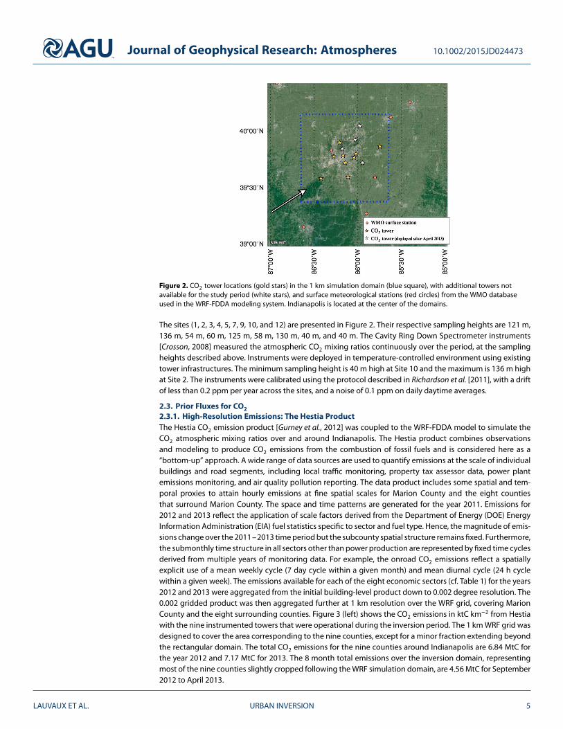
Figure 2. CO2 tower locations (gold stars) in the 1 km simulation domain (blue square), with additional towers notavailable for the study period (white stars), and surface meteorological stations (red circles) from the WMO databaseused in the WRF-FDDA modeling system. Indianapolis is located at the center of the domains.

The sites (1, 2, 3, 4, 5, 7, 9, 10, and 12) are presented in Figure 2. Their respective sampling heights are 121 m,136 m, 54 m, 60 m, 125 m, 58 m, 130 m, 40 m, and 40 m. The Cavity Ring Down Spectrometer instruments[Crosson, 2008] measured the atmospheric CO2 mixing ratios continuously over the period, at the samplingheights described above. Instruments were deployed in temperature-controlled environment using existingtower infrastructures. The minimum sampling height is 40 m high at Site 10 and the maximum is 136 m highat Site 2. The instruments were calibrated using the protocol described in Richardson et al. [2011], with a driftof less than 0.2 ppm per year across the sites, and a noise of 0.1 ppm on daily daytime averages.

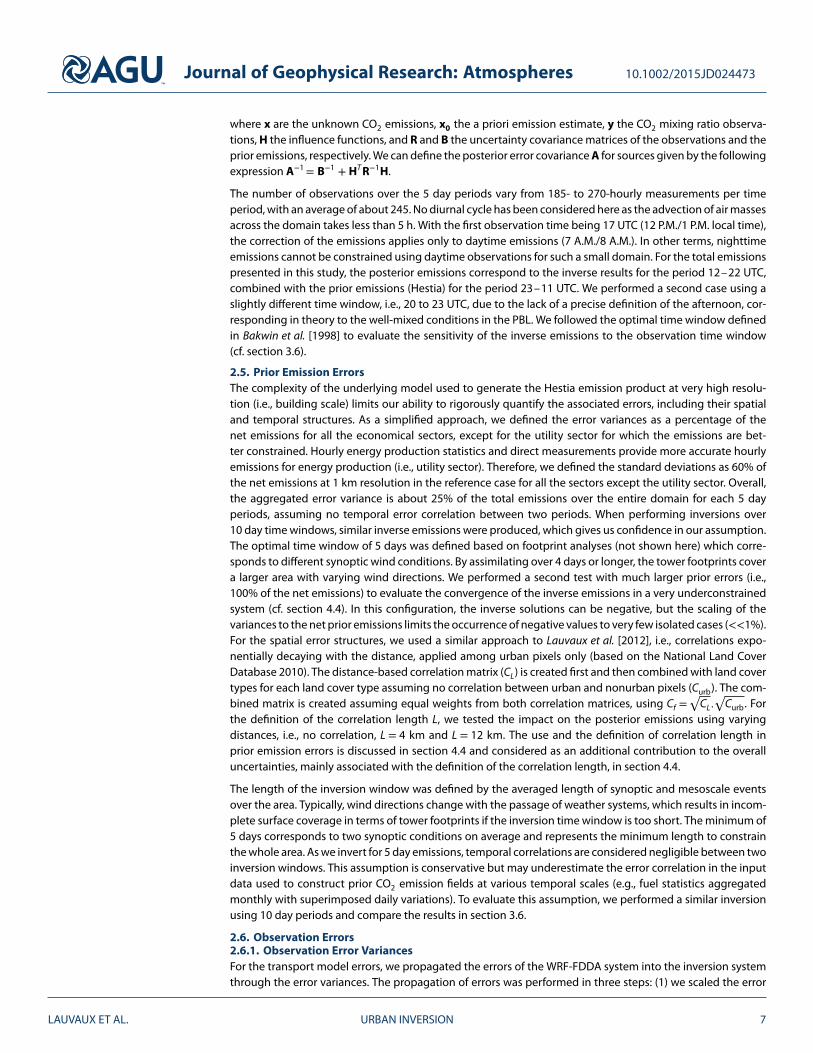
2.3. Prior Fluxes for CO22.3.1. High-Resolution Emissions: The Hestia ProductThe Hestia CO2 emission product [Gurney et al., 2012] was coupled to the WRF-FDDA model to simulate theCO2 atmospheric mixing ratios over and around Indianapolis. The Hestia product combines observationsand modeling to produce CO2 emissions from the combustion of fossil fuels and is considered here as a“bottom-up” approach. A wide range of data sources are used to quantify emissions at the scale of individualbuildings and road segments, including local traffic monitoring, property tax assessor data, power plantemissions monitoring, and air quality pollution reporting. The data product includes some spatial and tem-poral proxies to attain hourly emissions at fine spatial scales for Marion County and the eight countiesthat surround Marion County. The space and time patterns are generated for the year 2011. Emissions for2012 and 2013 reflect the application of scale factors derived from the Department of Energy (DOE) EnergyInformation Administration (EIA) fuel statistics specific to sector and fuel type. Hence, the magnitude of emis-sions change over the 2011–2013 time period but the subcounty spatial structure remains fixed. Furthermore,the submonthly time structure in all sectors other than power production are represented by fixed time cyclesderived from multiple years of monitoring data. For example, the onroad CO2 emissions reflect a spatiallyexplicit use of a mean weekly cycle (7 day cycle within a given month) and mean diurnal cycle (24 h cyclewithin a given week). The emissions available for each of the eight economic sectors (cf. Table 1) for the years2012 and 2013 were aggregated from the initial building-level product down to 0.002 degree resolution. The0.002 gridded product was then aggregated further at 1 km resolution over the WRF grid, covering MarionCounty and the eight surrounding counties. Figure 3 (left) shows the CO2 emissions in ktC km−2 from Hestiawith the nine instrumented towers that were operational during the inversion period. The 1 km WRF grid wasdesigned to cover the area corresponding to the nine counties, except for a minor fraction extending beyondthe rectangular domain. The total CO2 emissions for the nine counties around Indianapolis are 6.84 MtC forthe year 2012 and 7.17 MtC for 2013. The 8 month total emissions over the inversion domain, representingmost of the nine counties slightly cropped following the WRF simulation domain, are 4.56 MtC for September2012 to April 2013.



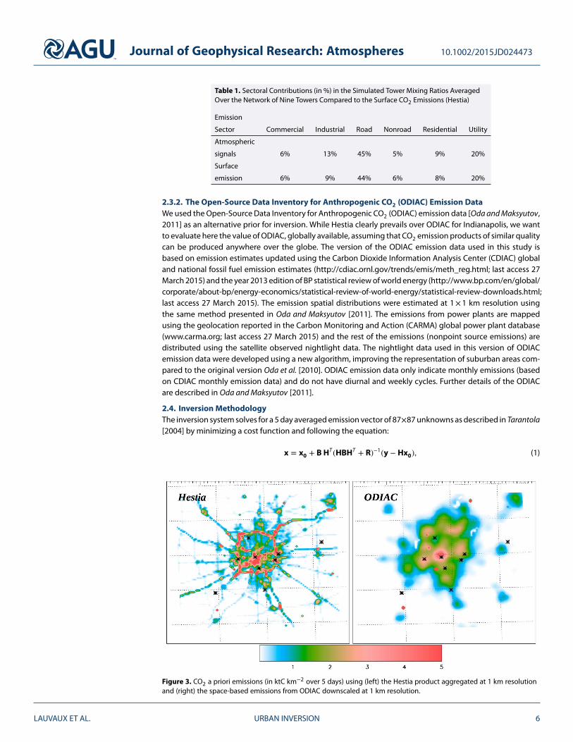
Table 1. Sectoral Contributions (in %) in the Simulated Tower Mixing Ratios AveragedOver the Network of Nine Towers Compared to the Surface CO2 Emissions (Hestia)

Emission

Sector Commercial Industrial Road Nonroad Residential Utility

Atmospheric

signals 6% 13% 45% 5% 9% 20%

Surface

emission 6% 9% 44% 6% 8% 20%

2.3.2. The Open-Source Data Inventory for Anthropogenic CO2 (ODIAC) Emission DataWe used the Open-Source Data Inventory for Anthropogenic CO2 (ODIAC) emission data [Oda and Maksyutov,2011] as an alternative prior for inversion. While Hestia clearly prevails over ODIAC for Indianapolis, we wantto evaluate here the value of ODIAC, globally available, assuming that CO2 emission products of similar qualitycan be produced anywhere over the globe. The version of the ODIAC emission data used in this study isbased on emission estimates updated using the Carbon Dioxide Information Analysis Center (CDIAC) globaland national fossil fuel emission estimates (http://cdiac.ornl.gov/trends/emis/meth_reg.html; last access 27March 2015) and the year 2013 edition of BP statistical review of world energy (http://www.bp.com/en/global/corporate/about-bp/energy-economics/statistical-review-of-world-energy/statistical-review-downloads.html;last access 27 March 2015). The emission spatial distributions were estimated at 1×1 km resolution usingthe same method presented in Oda and Maksyutov [2011]. The emissions from power plants are mappedusing the geolocation reported in the Carbon Monitoring and Action (CARMA) global power plant database(www.carma.org; last access 27 March 2015) and the rest of the emissions (nonpoint source emissions) aredistributed using the satellite observed nightlight data. The nightlight data used in this version of ODIACemission data were developed using a new algorithm, improving the representation of suburban areas com-pared to the original version Oda et al. [2010]. ODIAC emission data only indicate monthly emissions (basedon CDIAC monthly emission data) and do not have diurnal and weekly cycles. Further details of the ODIACare described in Oda and Maksyutov [2011].

2.4. Inversion MethodologyThe inversion system solves for a 5 day averaged emission vector of 87×87 unknowns as described in Tarantola[2004] by minimizing a cost function and following the equation:

x = x0 + B HT (HBHT + R)−1(y − Hx0), (1)

Figure 3. CO2 a priori emissions (in ktC km−2 over 5 days) using (left) the Hestia product aggregated at 1 km resolutionand (right) the space-based emissions from ODIAC downscaled at 1 km resolution.


http://cdiac.ornl.gov/trends/emis/meth_reg.html

http://www.bp.com/en/global/corporate/about-bp/energy-economics/statistical-review-of-world-energy/statistical-review-downloads.html

http://www.bp.com/en/global/corporate/about-bp/energy-economics/statistical-review-of-world-energy/statistical-review-downloads.html

http://www.carma.org


where x are the unknown CO2 emissions, x0 the a priori emission estimate, y the CO2 mixing ratio observa-tions, H the influence functions, and R and B the uncertainty covariance matrices of the observations and theprior emissions, respectively. We can define the posterior error covariance A for sources given by the followingexpression A−1 = B−1 + HT R−1H.

The number of observations over the 5 day periods vary from 185- to 270-hourly measurements per timeperiod, with an average of about 245. No diurnal cycle has been considered here as the advection of air massesacross the domain takes less than 5 h. With the first observation time being 17 UTC (12 P.M./1 P.M. local time),the correction of the emissions applies only to daytime emissions (7 A.M./8 A.M.). In other terms, nighttimeemissions cannot be constrained using daytime observations for such a small domain. For the total emissionspresented in this study, the posterior emissions correspond to the inverse results for the period 12–22 UTC,combined with the prior emissions (Hestia) for the period 23–11 UTC. We performed a second case using aslightly different time window, i.e., 20 to 23 UTC, due to the lack of a precise definition of the afternoon, cor-responding in theory to the well-mixed conditions in the PBL. We followed the optimal time window definedin Bakwin et al. [1998] to evaluate the sensitivity of the inverse emissions to the observation time window(cf. section 3.6).

2.5. Prior Emission ErrorsThe complexity of the underlying model used to generate the Hestia emission product at very high resolu-tion (i.e., building scale) limits our ability to rigorously quantify the associated errors, including their spatialand temporal structures. As a simplified approach, we defined the error variances as a percentage of thenet emissions for all the economical sectors, except for the utility sector for which the emissions are bet-ter constrained. Hourly energy production statistics and direct measurements provide more accurate hourlyemissions for energy production (i.e., utility sector). Therefore, we defined the standard deviations as 60% ofthe net emissions at 1 km resolution in the reference case for all the sectors except the utility sector. Overall,the aggregated error variance is about 25% of the total emissions over the entire domain for each 5 dayperiods, assuming no temporal error correlation between two periods. When performing inversions over10 day time windows, similar inverse emissions were produced, which gives us confidence in our assumption.The optimal time window of 5 days was defined based on footprint analyses (not shown here) which corre-sponds to different synoptic wind conditions. By assimilating over 4 days or longer, the tower footprints covera larger area with varying wind directions. We performed a second test with much larger prior errors (i.e.,100% of the net emissions) to evaluate the convergence of the inverse emissions in a very underconstrainedsystem (cf. section 4.4). In this configuration, the inverse solutions can be negative, but the scaling of thevariances to the net prior emissions limits the occurrence of negative values to very few isolated cases (<<1%).For the spatial error structures, we used a similar approach to Lauvaux et al. [2012], i.e., correlations expo-nentially decaying with the distance, applied among urban pixels only (based on the National Land CoverDatabase 2010). The distance-based correlation matrix (CL) is created first and then combined with land covertypes for each land cover type assuming no correlation between urban and nonurban pixels (Curb). The com-bined matrix is created assuming equal weights from both correlation matrices, using Cf =

√CL.

√Curb. For

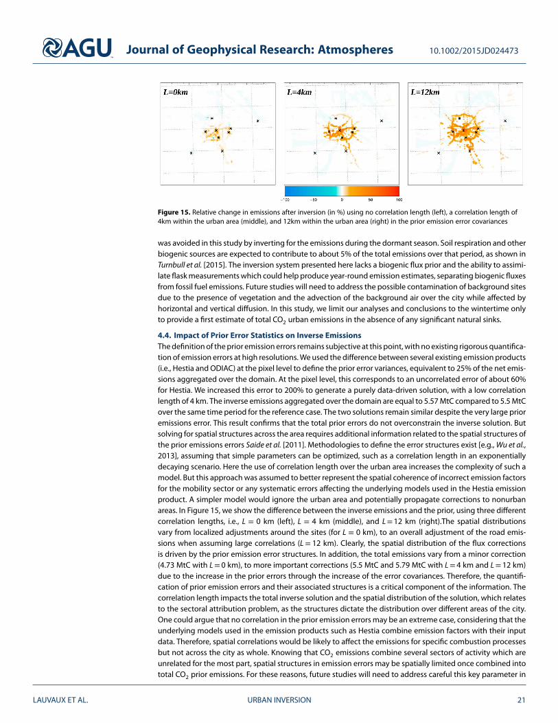
the definition of the correlation length L, we tested the impact on the posterior emissions using varyingdistances, i.e., no correlation, L = 4 km and L = 12 km. The use and the definition of correlation length inprior emission errors is discussed in section 4.4 and considered as an additional contribution to the overalluncertainties, mainly associated with the definition of the correlation length, in section 4.4.

The length of the inversion window was defined by the averaged length of synoptic and mesoscale eventsover the area. Typically, wind directions change with the passage of weather systems, which results in incom-plete surface coverage in terms of tower footprints if the inversion time window is too short. The minimum of5 days corresponds to two synoptic conditions on average and represents the minimum length to constrainthe whole area. As we invert for 5 day emissions, temporal correlations are considered negligible between twoinversion windows. This assumption is conservative but may underestimate the error correlation in the inputdata used to construct prior CO2 emission fields at various temporal scales (e.g., fuel statistics aggregatedmonthly with superimposed daily variations). To evaluate this assumption, we performed a similar inversionusing 10 day periods and compare the results in section 3.6.

2.6. Observation Errors2.6.1. Observation Error VariancesFor the transport model errors, we propagated the errors of the WRF-FDDA system into the inversion systemthrough the error variances. The propagation of errors was performed in three steps: (1) we scaled the error



variances using the normalized distance of a 𝜒2 distribution 𝜆 over each 5 day period. This first step providesan average variance for the period; (2) we adjust the variances for every hour using WRF-FDDA model perfor-mances for wind speed and direction; and (3) we readjust the variances by computing the normalized distanceof a 𝜒2 distribution for the second time 𝜆′. In the second step, we quantified the WRF-FDDA model perfor-mances (mean absolute errors (MAE)) for both wind speed and direction using the available surface WMOstations. This technique removes singular time steps during which the transport model performed poorly.

During the first step, the balance between prior error statistics and observation errors was evaluated usingthe 𝜒2 normalized distance 𝜆, defined by

𝜆 = 1n[(y − Hx0)T (H B HT + R)−1(y − Hx0)] (2)

similar to Kaminski et al. [2001].

For the second step, the hourly daytime MAE averaged over the domain, 𝜀, for the wind speed and direc-tion were used to define the hourly transport errors. Because these measurements were assimilated inthe WRF-FDDA simulation, the true MAE is most likely underestimated. However, we use these model-dataresiduals as a representation of the relative performances of the WRF-FDDA model at the hourly time scale. Inprinciple, meteorological errors cannot directly be diagnosed from modeled CO2 mixing ratios to describe theCO2 variances in the inversion. Indeed, both flux and transport errors affect the simulated CO2 mixing ratios.Instead, we only diagnosed transport errors from meteorological errors, which were then transformed intohourly scaling factors applied to hourly CO2 variances. To quantify these scaling factors, an error model wascreated to generate transport errors for the CO2 mixing ratios depending on both errors, i.e., in wind speedand direction. An adjustment coefficient defined as the ratio between the hourly MAE and the median of theMAE over the 5 day period was computed for both variables. The maximum of the two ratios define the hourlyadjustment coefficient. To avoid using the time steps during which the model is inaccurate, the hourly errorswere used to scale the variances 𝜀2

i,j for an observation (i) (i.e., the diagonal terms in R) using the followingrelationship:

𝜀2i = max

(𝜀spd

𝜇spd,𝜀dir

𝜇dir

)⋅ 𝜀2

init (3)

with 𝜀spd and 𝜀dir the hourly mean errors, 𝜇 the median of the 5 day errors, and 𝜀2init the initial variance from

step 1. We propagated the hourly transport model errors by using a multiplicative factor scaled with the per-formances of the modeled wind speed and direction. Over the inversion period (September 2012 to April2013), the median of the wind speed MAE is about 0.8 m s−1 and 12∘ for the wind direction. These two terms𝜇dir and 𝜇spd were used to provide a ratio between the averaged MAE and the hourly errors. A similar analysiswas performed on the wind direction. On an hourly basis, the ratio between the median and the hourly MAEwould define the adjustment of the initial error, e.g., multiplied by 2 for a wind speed MAE between 0.8 and1.6 m s−1, or by 3 between 1.6 to 2.4 m s−1, with no limit applied to the ratio. As described in equation (3), themaximum of the two variables (wind speed and direction) was used to define the final multiplicative factorapplied to the initial CO2 variance to adjust for incorrect wind direction or speed at any given time step, asdescribed in equation (3). In section 3.6, we compared this method to using a constant 𝜀i,j over time with nohourly adjustment based on the MAE.

The adjustment of the variances is computed from a 𝜒2 test (cf. section 2.4) using the normalized dis-tance 𝜆 over each 5 day periods [Tarantola, 2004]. For nondiagonal matrices, as described in the nextsection, the normalized distance 𝜆 correction cannot be applied directly to the variances and covariances;otherwise, the correction would be applied multiple times through the covariances and therefore overesti-mate the total errors. To compensate for the overestimation by the error covariances, we applied the squareroot of the scaling factor (

√𝜆.𝜀2

i,j) which assumes a linear relationship between variances and covariances(covx,y = corrx,y.𝜎x .𝜎y). This technique was tested over multiple 5 day segments and produced a systematicallybetter normalized distance 𝜆 (i.e., closer to one).2.6.2. Observation Error CorrelationsAt high resolutions, spatial and temporal correlations in transport model errors become increasinglyimportant. Past studies have approached the problem at coarser resolutions [e.g., Gerbig et al., 2003; Lauvauxet al., 2009a] and found that error covariances are significant when the distance between observation loca-tions is low. Using a diffusion equation model with an ensemble of transport simulations at 8 km resolution,



Lauvaux et al. [2009a] estimated the average correlation length in transport model errors at about 30–40 km.Between the INFLUX towers, the average distance is about 40 km, which suggests that spatial error correla-tions may be significant. However, the correlation length may vary in space and time and is likely to dependon model resolution and physics. To evaluate the sensitivity of the inverse emissions to spatial error correla-tions, we assumed a relatively small correlation length and an exponentially decaying model for the distance,with Lobs =10 km, following the equation:

Ci,jobs = exp

−d2

i,j

L2obs (4)

with Ci,jobs the correlation coefficient between two tower locations i and j and di,j the distance between the

towers i and j. The observation error correlation matrix Cobs has to be symetric, positive semidefinite, with thediagonal terms equal to one. Further investigations of Cobs showed that a small number of eigenvalues werenegative and required some modifications of the initial matrix before inversion. Following Brissette et al. [2007],we used an iterative process to filter negative eigenvalues. The negative values were replaced by slightly pos-itive eigenvalues, and the correlation matrix was regenerated using the original eigenvectors. The matrix wasslightly modified to be symmetric and with positive correlations only. The iterative process converged for allthe inversion periods, modifying the correlation by less than 10%.

Temporal error correlations at high frequency (i.e., hourly) can also affect the simulated atmospheric mixingratios [Lauvaux et al., 2009a]. However, the batch inversion system as defined here is less affected by the impactof hourly error correlations, as the atmospheric data are assimilated in a single block. Spatially, emission cor-rections may still vary, but the overall city-wide emissions are unlikely to be affected. Further investigationsof temporal error correlations in the observations are needed to better quantify their impact on the inversesolution. Here no temporal correlation was introduced in the errors. We quantified the impact of spatial errorcorrelations by performing a sensitivity study, comparing the impact of error correlation, i.e., nondiagonalterms in R to the reference configuration in section 2.6.2. Further investigation is required to define morecompletely the spatial and temporal error correlations in high-resolution transport simulations and theirimpact on the inverse emissions, similar to Lauvaux et al. [2009a] at coarser resolution.

2.7. Boundary Inflow: Data SelectionThe constant flow of air through the boundaries of a limited-domain atmospheric simulation represents asignificant amount of carbon compared to the local emissions and therefore is a critical quantity that has tobe characterized in the inversion system [Göckede et al., 2010; Lauvaux et al., 2012]. Several studies have sug-gested to simply measure this quantity upwind of the metropolitan area [Kort et al., 2012; McKain et al., 2012]similar to aircraft mass balance techniques [Cambaliza et al., 2014; Karion et al., 2015]. However, backgroundmeasurements can be affected by local fluxes and/or the local atmospheric dynamics which would impair itsspatial representativity as a background measurement. The inflow of air follows primarily the wind directionand its variability in time and space, directly affecting our ability to measure the upwind conditions in anymeteorological situations. Therefore, no measured background concentration would remain constant as theair moves across the domain. Advection-diffusion and vertical mixing modify the mixing ratios as air massesmove over the city, increasing the representation errors associated with upwind measurements.

To measure the background air, the initial design of the Influx network included two sites covering the twomajor wind directions in the area, i.e., Site 1 for the northwesterly through westerly flows and Site 9 fornortherly through easterly winds. We compared several sites of the network (i.e., Sites 1, 4, 5, and 9) bycomputing the fraction of days corresponding to low atmospheric concentrations for each site. This analysisassumes that cleaner air should be measured at the background sites. The results indicate that Site 1 shows thelowest concentrations on average over time, whereas Site 9 is systematically higher by a couple tenths of appm. Sites 4 and 5 are clearly influenced by local emissions and should not be used as background sites.

We selected Sites 1 and 9 as our least biased background sites for our analysis and defined the backgroundconcentration for each hourly measurement over Indianapolis following different scenarios. These scenarioscorrespond to the definition of the upwind concentrations at a given time, or under specific conditions. Toevaluate the impact of the definition of the boundary conditions on the inverse emissions, we producedseveral inverse emissions using different selection methods. First, we used a fixed site for the entire inver-sion period, using the hourly concentrations at the exact hour. This scenario is the simplest option for limitednetworks of towers. Second, we used an upwind model, selecting the sites based on the hourly surface wind



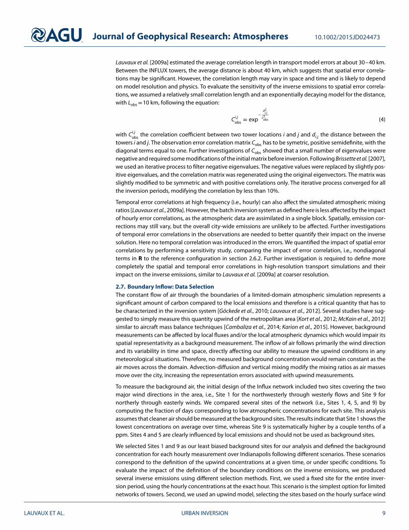
Figure 4. Selection of the background site to determine the upwind concentrations of CO2 over Indianapolis, usingtwo semicircles (135∘ and 315∘) and hourly modeled wind directions from the WRF-FDDA system at three locationsacross the city. The emitting area defined by Hestia is represented in gray. The distance between Site 1 and Site 9(about 35 km) corresponds to an advection time of about 2 h. The wind climatology for the month of December atthe Indianapolis airport (IND station) is shown under the legend (in red).

direction in the center of Indianapolis. The upwind model selected Site 1 when the wind was between 135∘

and 315∘ and Site 9 for 315∘ to 135∘ (cf. Figure 4). Third, we used a daily minimum measured across thenetwork to evaluate the importance of hourly changes. The results are presented in section 3.5. Additionalerrors could still affect the background sites such as local biogenic signals from soil respiration which arenonnegligible even in wintertime in midlatitudes [cf. Pataki et al., 2007]. A third background tower is beingdeployed in a different area to address more carefully the possible local biogenic fluxes mixed with large-scalegradients in atmospheric mixing ratios advected over the city.

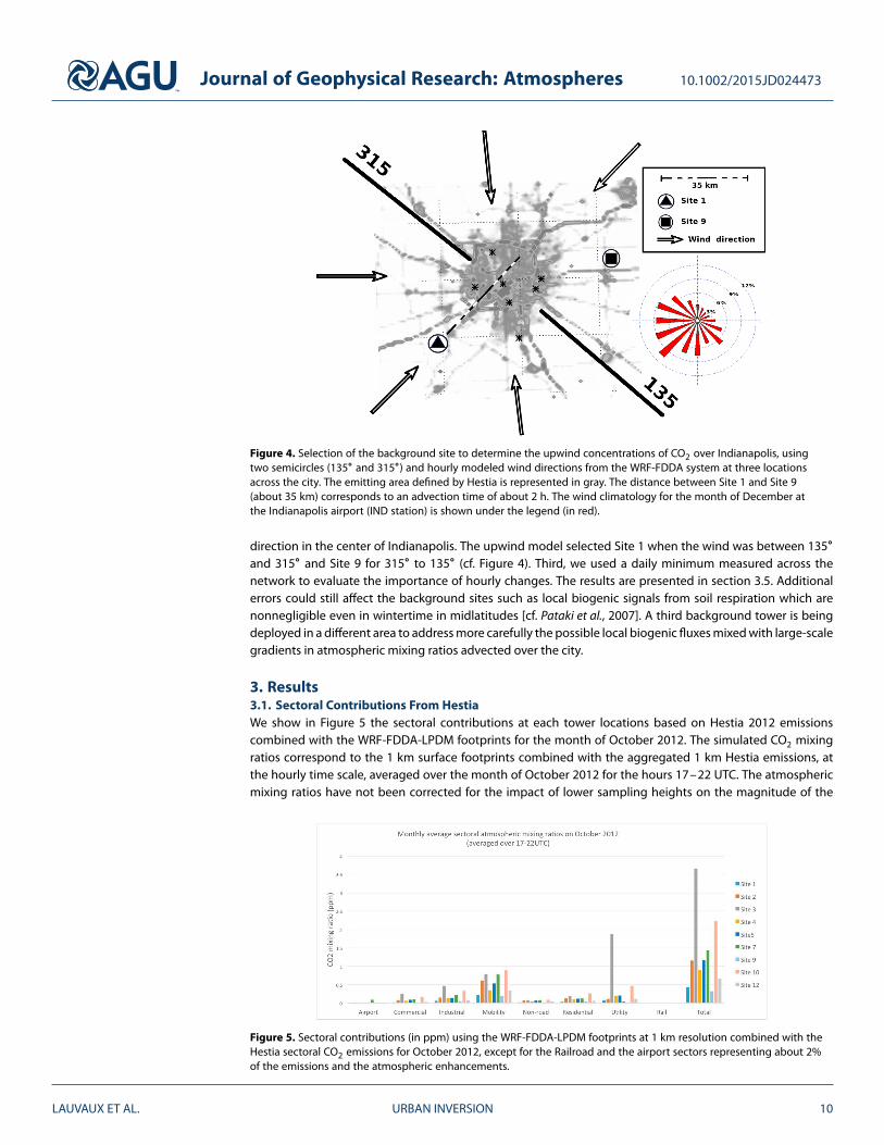
3. Results3.1. Sectoral Contributions From HestiaWe show in Figure 5 the sectoral contributions at each tower locations based on Hestia 2012 emissionscombined with the WRF-FDDA-LPDM footprints for the month of October 2012. The simulated CO2 mixingratios correspond to the 1 km surface footprints combined with the aggregated 1 km Hestia emissions, atthe hourly time scale, averaged over the month of October 2012 for the hours 17–22 UTC. The atmosphericmixing ratios have not been corrected for the impact of lower sampling heights on the magnitude of the

Figure 5. Sectoral contributions (in ppm) using the WRF-FDDA-LPDM footprints at 1 km resolution combined with theHestia sectoral CO2 emissions for October 2012, except for the Railroad and the airport sectors representing about 2%of the emissions and the atmospheric enhancements.



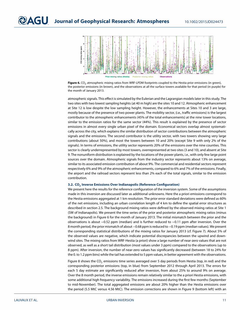
Figure 6. CO2 atmospheric mixing ratios from WRF-LPDM footprints coupled to the Hestia prior emissions (in green),the posterior emissions (in brown), and the observations at all the surface towers available for that period (in purple) forthe month of January 2013.

atmospheric signals. This effect is simulated by the Eulerian and the Lagrangian models later in this study. Thetwo sites with two lowest sampling heights (at 40 m high) are the sites 10 and 12. Atmospheric enhancementat Site 12 is low despite the low sampling height. However, the enhancements at Sites 10 and 3 are large,mostly because of the presence of two power plants. The mobility sector, (i.e., traffic emissions) is the largestcontributor to the atmospheric enhancements (45% of the total enhancements) at the nine tower locations,similar to the emission ratios for the same sector (44%). This result is explained by the presence of sectoremissions in almost every single urban pixel of the domain. Economical sectors overlap almost systemati-cally across the city, which explains the similar distribution of sector contributions between the atmosphericsignals and the emissions. The second contributor is the utility sector, with two towers showing very largecontributions (about 50%), and most the towers between 10 and 20% (except Site 9 with only 2% of thesignals). In terms of emissions, the utility sector represents 20% of the emissions over the nine counties. Thissector is clearly underrepresented by most towers, overrepresented at two sites (3 and 10), and absent at Site9. The nonuniform distribution is explained by the locations of the power plants, i.e., with only few large pointsources over the domain. Atmospheric signals from the industry sector represents about 13% on average,similar to its associated emission contribution of about 9%. The commercial and residential sectors representrespectively 6% and 9% of the atmospheric enhancements, compared to 6% and 7% of the emissions. Finally,the airport and the railroad sectors represent less than 2% each of the total signals, similar to the emissioncontribution.

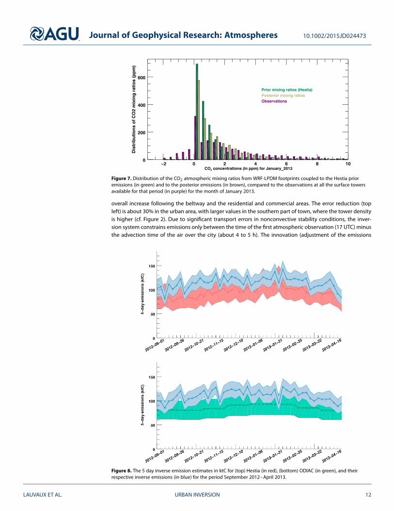
3.2. CO2 Inverse Emissions Over Indianapolis (Reference Configuration)We present here the results for the reference configuration of the inversion system. Some of the assumptionsmade in this inversion are discussed later as additional unknowns. Here the a priori emissions correspond tothe Hestia emissions aggregated at 1 km resolution. The prior error standard deviations were defined as 60%of the net emissions, including an urban correlation length of 4 km to define the spatial error structures asdescribed in section 2.5. The background mixing ratios were defined by the observed mixing ratios at Site 1(SW of Indianapolis). We present the time series of the prior and posterior atmospheric mixing ratios (minusthe background) in Figure 6 for the month of January 2013. The initial mismatch between the prior and theobservations is about −0.52 ppm (median) and is further reduced to −0.11 ppm after inversion. Over the8 month period, the prior mismatch of about−0.68 ppm is reduced to−0.19 ppm (median values). We presentthe corresponding statistical distributions of the mixing ratios for January 2013 (cf. Figure 7). About 5% ofthe observed values are negative, which indicate potential discrepancies between the upwind and down-wind sites. The mixing ratios from WRF-Hestia (a priori) show a large number of near-zero values that are notobserved, as well as a short tail distribution (most values under 3 ppm) compared to the observations (up to8 ppm). After inversion, the number of near-zero values has significantly decreased (between 18 to 24% forthe 0. to 1.2 ppm bins) while the tail has extended to 5 ppm values, in better agreement with the observations.

Figure 8 shows the CO2 emissions time series averaged over 5 day periods from Hestia (top, in red) and thecorresponding posterior emissions (top, in blue) from September 2012 through April 2013. The errors foreach 5 day estimate are significantly reduced after inversion, from about 25% to around 9% on average.Over the 8 month period, the inverse emissions remain relatively similar to the a priori Hestia emissions, withsome additional high frequency variability. The emissions increased during the first few months (Septemberto mid-November). The total aggregated emissions are about 20% higher than the Hestia emissions overthe period (5.5 MtC versus 4.56 MtC). The emission corrections are shown in Figure 9 (bottom left) with an



Figure 7. Distribution of the CO2 atmospheric mixing ratios from WRF-LPDM footprints coupled to the Hestia prioremissions (in green) and to the posterior emissions (in brown), compared to the observations at all the surface towersavailable for that period (in purple) for the month of January 2013.

overall increase following the beltway and the residential and commercial areas. The error reduction (topleft) is about 30% in the urban area, with larger values in the southern part of town, where the tower densityis higher (cf. Figure 2). Due to significant transport errors in nonconvective stability conditions, the inver-sion system constrains emissions only between the time of the first atmospheric observation (17 UTC) minusthe advection time of the air over the city (about 4 to 5 h). The innovation (adjustment of the emissions

Figure 8. The 5 day inverse emission estimates in ktC for (top) Hestia (in red), (bottom) ODIAC (in green), and theirrespective inverse emissions (in blue) for the period September 2012–April 2013.



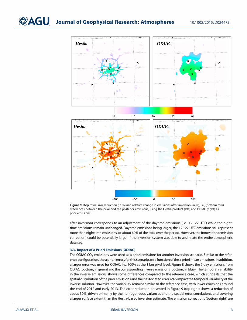
Figure 9. (top row) Error reduction (in %) and relative change in emissions after inversion (in %), i.e., (bottom row)differences between the prior and the posterior emissions, using the Hestia product (left) and ODIAC (right) asprior emissions.

after inversion) corresponds to an adjustment of the daytime emissions (i.e., 12–22 UTC) while the night-time emissions remain unchanged. Daytime emissions being larger, the 12–22 UTC emissions still representmore than nighttime emissions, or about 60% of the total over the period. However, the innovation (emissioncorrection) could be potentially larger if the inversion system was able to assimilate the entire atmosphericdata set.

3.3. Impact of a Priori Emissions (ODIAC)The ODIAC CO2 emissions were used as a priori emissions for another inversion scenario. Similar to the refer-ence configuration, the a priori errors for this scenario are a function of the a priori mean emissions. In addition,a larger error was used for ODIAC, i.e., 100% at the 1 km pixel level. Figure 8 shows the 5 day emissions fromODIAC (bottom, in green) and the corresponding inverse emissions (bottom, in blue). The temporal variabilityin the inverse emissions shows some differences compared to the reference case, which suggests that thespatial distribution of the prior emissions and their associated errors can impact the temporal variability of theinverse solution. However, the variability remains similar to the reference case, with lower emissions aroundthe end of 2012 and early 2013. The error reduction presented in Figure 9 (top right) shows a reduction ofabout 30%, driven primarily by the homogeneous variances and the spatial error correlations, and coveringa larger surface extent than the Hestia-based inversion estimate. The emission corrections (bottom right) are



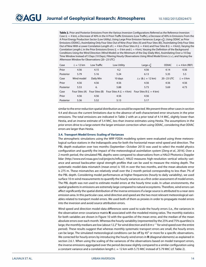
Table 2. Prior and Posterior Emissions From the Various Inversion Configurations Referred as the Reference InversionCase (L = 4 km), a Decrease of 40% in the A Priori Traffic Emissions (Low Traffic), a Decrease of 40% in Emissions From theA Priori Energy Production Sector (Low Utility), Using Large Prior Emission Variances (Large 𝜎2

B ), Using ODIAC as PriorEmissions (ODIAC), Assimilating Only Four Sites Out of Nine (Four Sites (A) and Four Sites (B)), Assimilating Only Four SitesOut of Nine With a Lower Correlation Length of L = 4 km (Four Sites A (L = 4 km) and Four Sites B (L = 4 km)), Varying theCorrelation Length L in the Prior Emissions Errors (L = 0 km and L = 4 km), Varying the Definition of the BackgroundConditions Using the Wind Direction (Wind Model) or the Minimum of the Day (Daily Min), Assimilating Over a 10 DayTime Window Instead of 5 Days (10 Days), Filtering Hourly Observations Using Wind Model Errors (𝜆.𝜀), and Varying theAfternoon Window for Observations (20–23 UTC)

Case L = 12 km Low Traffic Low Utility Large 𝜎2B ODIAC L = 4 km (REF)

Prior 4.56 4.15 4.2 4.56 4.14 4.56

Posterior 5.79 5.16 5.24 6.13 5.35 5.5

Case Wind model Daily Min 10 days 𝜆.𝜀 (& L = 12 km) 20–23 UTC L = 0 km

Prior 4.56 4.56 4.56 4.56 4.56 4.56

Posterior 5.53 6. 5.88 5.73 5.69 4.73

Case Four Sites (A) Four Sites (B) Four Sites A (L = 4 km) Four Sites B (L = 4 km)

Prior 4.56 4.56 4.56 4.56

Posterior 5.36 5.52 5.13 5.17

similar to the error reduction spatial distribution as would be expected. We present three other cases in section4.4 and discuss the current limitations due to the absence of well-characterized error structures in the prioremissions. The total emissions are indicated in Table 2 with an a prior total of 4.14 MtC, slightly lower thanHestia, and an inverse estimate of 5.4 MtC, less than inverse estimates using Hestia. The assumptions in theprior errors drive to a large extent the larger emission correction when using ODIAC, considering that ODIACerrors are larger than Hestia.

3.4. Transport Model Errors: Scaling of VariancesThe atmospheric simulations using the WRF-FDDA modeling system were evaluated using three meteoro-logical surface stations in the Indianapolis area for both the horizontal mean wind speed and direction. ThePBL depth evaluation over two months (September–October 2013) was used to select the model physicsconfiguration and quantify the impact of the meteorological assimilation system [Deng et al., 2016]. Over a2 month period, the simulated PBL depths were compared to observations from a HALO Photonics Dopplerlidar (http://www.esrl.noaa.gov/csd/projects/influx/). HALO measures high-resolution vertical velocity vari-ance and aerosol backscatter signal strength profiles that can be used to measure the mixing depth. Thesystematic model-data mismatch (mean error) is 105 m over the two months, and the mean absolute erroris 275 m. These mismatches are relatively small over the 2 month period corresponding to less than 7% ofthe PBL depth. Considering model performances at higher frequencies (hourly to daily variability), we usedsurface 10 m wind measurements to quantify the hourly variances as a first-order assessment of model errors.The PBL depth was not used to estimate model errors at the hourly time scale. In urban environments, thespatial gradients in emissions are extremely large compared to natural ecosystems. Therefore, wind errors canaffect significantly the spatial distribution of the inverse emissions if a large source is attributed to a near-zeroemission area. In this particular case, wind direction and speed are the two most relevant meteorological vari-ables related to transport model errors. We used both of them as proxies in order to propagate model errorsinto the inversion and avoid source attribution errors.

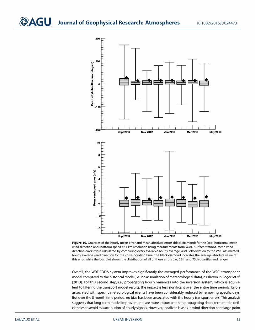
Wind speed and direction model-data differences were used to scale the hourly errors (i.e., the variances inthe observation error covariance matrix R) associated with the modeled mixing ratios. The monthly statisticsfor both variables are shown in Figure 10 with the quartiles of the mean error, and the median of the meanabsolute errors over each month. Whereas the hourly variability (represented by the 25% and 75% quartiles) islarge, the monthly medians are low (about 12.2∘ for wind direction and 0.8 m s−1 for wind speed over the entireperiod). These results suggest that whereas monthly systematic transport errors are small, the hourly errorscan be large. The simulated meteorological conditions can be off by 45∘ or more for a specific observations.We corrected for hourly errors by introducing the hourly wind errors in R (diagonal elements) as explained insection 2.6.1. When using the scaling of the variances of the observations based on model transport errors,the inverse emissions aggregated over the period decrease slightly compared to a similar configuration usinga constant variance and a correlation length L = 12 km with 5.73 MtC instead of 5.79 MtC (cf. Table 2).


http://www.esrl.noaa.gov/csd/projects/influx/


Figure 10. Quartiles of the hourly mean error and mean absolute errors (black diamond) for the (top) horizontal meanwind direction and (bottom) speed at 1 km resolution using measurements from WMO surface stations. Mean winddirection errors were calculated by comparing every available hourly average WMO observation to the WRF-assimilatedhourly average wind direction for the corresponding time. The black diamond indicates the average absolute value ofthis error while the box plot shows the distribution of all of these errors (i.e., 25th and 75th quartiles and range).

Overall, the WRF-FDDA system improves significantly the averaged performance of the WRF atmosphericmodel compared to the historical mode (i.e., no assimilation of meteorological data), as shown in Rogers et al.[2013]. For this second step, i.e., propagating hourly variances into the inversion system, which is equiva-lent to filtering the transport model results, the impact is less significant over the entire time periods. Errorsassociated with specific meteorological events have been considerably reduced by removing specific days.But over the 8 month time period, no bias has been associated with the hourly transport errors. This analysissuggests that long-term model improvements are more important than propagating short-term model defi-ciencies to avoid misattribution of hourly signals. However, localized biases in wind direction near large point



sources could have a significant impact on the modeled mixing ratios for specific towers. We only consideredthe long-term average over the city and ignored local effects which would require high-resolution modelingof local plumes.

3.5. Sensitivity to the Background ConcentrationsWe present here the results of the different strategies used to define the background concentrations.Compared to previous regional inversion studies [e.g., Göckede et al., 2010; Lauvaux et al., 2012], the boundaryconditions were directly sampled upwind of the tower network, which provides accurate measurements butis potentially less representative than spatially resolved modeled concentrations. However, considering themagnitude of the city enhancement (i.e., about 3 ppm at the downtown site), current regional models wouldfail to provide sufficient accuracy over the city, as shown by Bréon et al. [2015]. At larger scales (i.e., 10 km),Lauvaux et al. [2012] estimated that the long-term bias from the model atmospheric mole fractions of Carbon-Tracker [Peters et al., 2007] was around 0.5 ppm, with daily errors from 1 to 7 ppm depending on the season.Here the first strategy defines the background concentrations by using the concentrations at Site 1 at the exacttime of the observations. Site 1 is the climatological background site located upwind about 60% of the time(cf. Figure 4). The second strategy uses the optimal site location based on the wind direction (upwind model),as described earlier. Sites 1 and 9 are the two options depending on the wind direction. When one site is notoperational, the other is used even if the wind direction is not optimal. Over the 8 month period, Site 1 wasoperational about 65% of the time, while Site 9 was measuring more than 90% of the time. The last strategyuses the daily minimum at the upwind site, similar to the second strategy. This last option offset potentialtemporal variations observed in the early afternoon. The risk of sampling low concentrations at later times isnot negligible. This strategy is the least likely option for realistically sampling the background. Table 2 showsthat the two first strategies produce very similar inverse total emissions with 5.53 MtC (wind model) and5.5 MtC (L = 4 km), whereas the third strategy increases the total emissions significantly (6 MtC). The dailyminimums are selected over the time window 17–22 UTC, with the lowest values being usually observedbetween 20 and 22 UTC. This technique introduces a positive bias in the inverse solution by selecting lateafternoon mixing ratios at the upwind site (i.e., lower concentrations), artificially increasing the emissionsover the city. This last method is the least realistic because the lowest concentrations are often observed atthe end of the day, which is inconsistent with the advection time of air masses across the city. The first twostrategies represent the difference between Site 1 and a combination of Sites 1 and 9 depending on the winddirection. If Site 1 is contaminated by any local signals, the current analysis would not diagnose its impact.An additional site measuring background concentrations will be deployed to test the potential impact ofupwind sources.

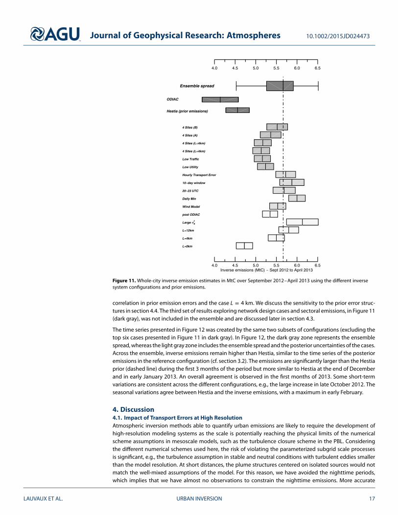
3.6. Uncertainty Assessment: Ensemble Approach of Inverse EstimatesAn ensemble approach of inversion configurations was designed to quantify systematic errors due to thevarious assumptions made in the urban inversion system. The ensemble consists of two sets of results, thefirst representing prior-related cases, such as varying the spatial error structures in prior emission errors, andthe second set of results related to the observations and their associated uncertainties. The first set of results,presented in Figure 11 (light gray), shows three different correlation lengths L (as described in section 2.5)and a different prior (ODIAC). The impact of various L is clearly the main contributor to the changes in totalemissions, even if the fully uncorrelated prior emission scenario seems very unlikely considering the use ofdata and model parameters in the Hestia and ODIAC products. We discuss the impact of L on the spatial distri-bution and the total emissions in section 4.4. The use of ODIAC is also important with noticeable differencesin the spatial distribution. The second set of results, in gray, includes different assumptions related to the timewindow for the observations (20–23 UTC instead of 17–22 UTC). We defined the well-mixed conditionsbased on the temporal variability in the CO2 mixing ratios and found that the period 20–23 UTC would bemore appropriate to avoid a late morning transition in the PBL depth. The results are presented in Table 2.The difference with the reference case remains small which may suggest that the WRF-FDDA model is ableto simulate the late PBL growth in the early afternoon. The ensemble includes several other configura-tions including the use of hourly transport errors based on hourly wind error statistics, and the definitionof the background concentrations. The two sets were used to define the quartiles of the ensemble, notedensemble spread in Figure 11. The ensemble mean is about 5.66 MtC, the second and third quartiles at 0.23 MtCfrom the mean, the first and fourth quartiles at 0.85 MtC from the mean. The inverse emission using Hes-tia and ODIAC are statistically different from the 50–75% of the ensemble mean. However, the definitionof the correlation length seems to encompass both prior and posterior solutions, especially between no



Figure 11. Whole-city inverse emission estimates in MtC over September 2012–April 2013 using the different inversesystem configurations and prior emissions.

correlation in prior emission errors and the case L = 4 km. We discuss the sensitivity to the prior error struc-tures in section 4.4. The third set of results exploring network design cases and sectoral emissions, in Figure 11(dark gray), was not included in the ensemble and are discussed later in section 4.3.

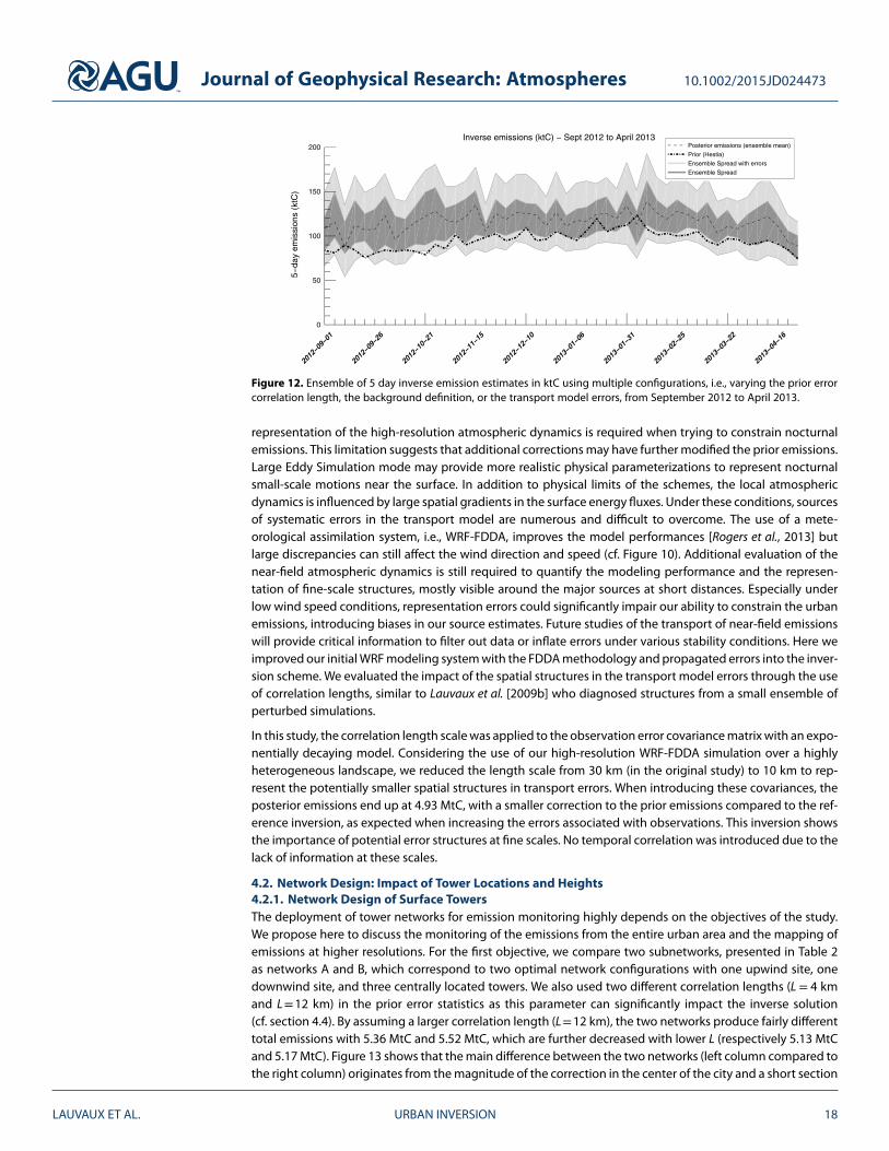
The time series presented in Figure 12 was created by the same two subsets of configurations (excluding thetop six cases presented in Figure 11 in dark gray). In Figure 12, the dark gray zone represents the ensemblespread, whereas the light gray zone includes the ensemble spread and the posterior uncertainties of the cases.Across the ensemble, inverse emissions remain higher than Hestia, similar to the time series of the posterioremissions in the reference configuration (cf. section 3.2). The emissions are significantly larger than the Hestiaprior (dashed line) during the first 3 months of the period but more similar to Hestia at the end of Decemberand in early January 2013. An overall agreement is observed in the first months of 2013. Some short-termvariations are consistent across the different configurations, e.g., the large increase in late October 2012. Theseasonal variations agree between Hestia and the inverse emissions, with a maximum in early February.

4. Discussion4.1. Impact of Transport Errors at High ResolutionAtmospheric inversion methods able to quantify urban emissions are likely to require the development ofhigh-resolution modeling systems as the scale is potentially reaching the physical limits of the numericalscheme assumptions in mesoscale models, such as the turbulence closure scheme in the PBL. Consideringthe different numerical schemes used here, the risk of violating the parameterized subgrid scale processesis significant, e.g., the turbulence assumption in stable and neutral conditions with turbulent eddies smallerthan the model resolution. At short distances, the plume structures centered on isolated sources would notmatch the well-mixed assumptions of the model. For this reason, we have avoided the nighttime periods,which implies that we have almost no observations to constrain the nighttime emissions. More accurate



Figure 12. Ensemble of 5 day inverse emission estimates in ktC using multiple configurations, i.e., varying the prior errorcorrelation length, the background definition, or the transport model errors, from September 2012 to April 2013.

representation of the high-resolution atmospheric dynamics is required when trying to constrain nocturnalemissions. This limitation suggests that additional corrections may have further modified the prior emissions.Large Eddy Simulation mode may provide more realistic physical parameterizations to represent nocturnalsmall-scale motions near the surface. In addition to physical limits of the schemes, the local atmosphericdynamics is influenced by large spatial gradients in the surface energy fluxes. Under these conditions, sourcesof systematic errors in the transport model are numerous and difficult to overcome. The use of a mete-orological assimilation system, i.e., WRF-FDDA, improves the model performances [Rogers et al., 2013] butlarge discrepancies can still affect the wind direction and speed (cf. Figure 10). Additional evaluation of thenear-field atmospheric dynamics is still required to quantify the modeling performance and the represen-tation of fine-scale structures, mostly visible around the major sources at short distances. Especially underlow wind speed conditions, representation errors could significantly impair our ability to constrain the urbanemissions, introducing biases in our source estimates. Future studies of the transport of near-field emissionswill provide critical information to filter out data or inflate errors under various stability conditions. Here weimproved our initial WRF modeling system with the FDDA methodology and propagated errors into the inver-sion scheme. We evaluated the impact of the spatial structures in the transport model errors through the useof correlation lengths, similar to Lauvaux et al. [2009b] who diagnosed structures from a small ensemble ofperturbed simulations.

In this study, the correlation length scale was applied to the observation error covariance matrix with an expo-nentially decaying model. Considering the use of our high-resolution WRF-FDDA simulation over a highlyheterogeneous landscape, we reduced the length scale from 30 km (in the original study) to 10 km to rep-resent the potentially smaller spatial structures in transport errors. When introducing these covariances, theposterior emissions end up at 4.93 MtC, with a smaller correction to the prior emissions compared to the ref-erence inversion, as expected when increasing the errors associated with observations. This inversion showsthe importance of potential error structures at fine scales. No temporal correlation was introduced due to thelack of information at these scales.

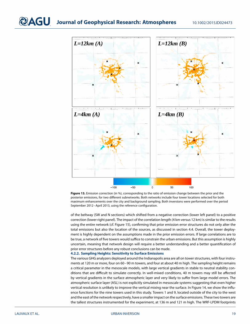
4.2. Network Design: Impact of Tower Locations and Heights4.2.1. Network Design of Surface TowersThe deployment of tower networks for emission monitoring highly depends on the objectives of the study.We propose here to discuss the monitoring of the emissions from the entire urban area and the mapping ofemissions at higher resolutions. For the first objective, we compare two subnetworks, presented in Table 2as networks A and B, which correspond to two optimal network configurations with one upwind site, onedownwind site, and three centrally located towers. We also used two different correlation lengths (L = 4 kmand L=12 km) in the prior error statistics as this parameter can significantly impact the inverse solution(cf. section 4.4). By assuming a larger correlation length (L=12 km), the two networks produce fairly differenttotal emissions with 5.36 MtC and 5.52 MtC, which are further decreased with lower L (respectively 5.13 MtCand 5.17 MtC). Figure 13 shows that the main difference between the two networks (left column compared tothe right column) originates from the magnitude of the correction in the center of the city and a short section



Figure 13. Emission correction (in %), corresponding to the ratio of emission change between the prior and theposterior emissions, for two different subnetworks. Both networks include four tower locations selected for bothmaximum enhancements over the city and background sampling. Both inversions were performed over the periodSeptember 2012–April 2013, using the reference configuration.

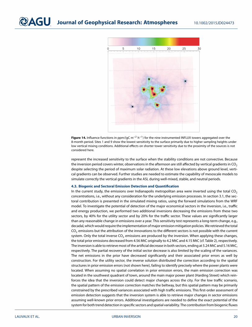
of the beltway (SW and N sections) which shifted from a negative correction (lower left panel) to a positivecorrection (lower right panel). The impact of the correlation length (4 km versus 12 km) is similar to the resultsusing the entire network (cf. Figure 15), confirming that prior emission error structures do not only alter thetotal emissions but also the location of the sources, as discussed in section 4.4. Overall, the tower deploy-ment is highly dependent on the assumptions made in the prior emission errors. If large correlations are tobe true, a network of five towers would suffice to constrain the urban emissions. But this assumption is highlyuncertain, meaning that network design will require a better understanding and a better quantification ofprior error structures before any robust conclusions can be made.4.2.2. Sampling Heights: Sensitivity to Surface EmissionsThe various GHG analyzers deployed around the Indianapolis area are all on tower structures, with four instru-ments at 120 m or more, four on 60–90 m towers, and four at about 40 m high. The sampling height remainsa critical parameter in the mesoscale models, with large vertical gradients in stable to neutral stability con-ditions that are difficult to simulate correctly. In well-mixed conditions, 40 m towers may still be affectedby vertical gradients in the surface atmospheric layer and very likely to suffer from large model errors. Theatmospheric surface layer (ASL) is not explicitly simulated in mesoscale systems suggesting that even highervertical resolution is unlikely to improve the vertical mixing near the surface. In Figure 14, we show the influ-ence functions for the nine towers used in this study. Towers 1 and 9, located outside of the city to the westand the east of the network respectively, have a smaller impact on the surface emissions. These two towers arethe tallest structures instrumented for the experiment, at 136 m and 121 m high. The WRF-LPDM footprints



Figure 14. Influence functions in ppm/(gC m−2 h−1) for the nine instrumented INFLUX towers aggregated over the8-month period. Sites 1 and 9 show the lowest sensitivity to the surface primarily due to higher sampling heights underlow vertical mixing conditions. Additional effects on shorter tower sensitivity due to the proximity of the sources is notconsidered here.

represent the increased sensitivity to the surface when the stability conditions are not convective. Becausethe inversion period covers winter, observations in the afternoon are still affected by vertical gradients in CO2

despite selecting the period of maximum solar radiation. At these low elevations above ground level, verti-cal gradients can be observed. Further studies are needed to estimate the capability of mesoscale models tosimulate correctly the vertical gradients in the ASL during well-mixed, stable, and neutral periods.

4.3. Biogenic and Sectoral Emission Detection and QuantificationIn the current study, the emissions over Indianapolis metropolitan area were inverted using the total CO2

concentrations, i.e., without any consideration for the underlying emission processes. In section 3.1, the sec-toral contribution is presented in the simulated mixing ratios, using the forward simulations from the WRFmodel. To investigate the potential of detection of the major economical sectors in the inversion, i.e., trafficand energy production, we performed two additional inversions decreasing the emissions from these twosectors, by 40% for the utility sector and by 20% for the traffic sector. These values are significantly largerthan any reasonable change in emissions over a year. This sensitivity test represents a long-term change, e.g.,decadal, which would require the implementation of major emission mitigation policies. We retrieved the totalCO2 emissions but the attribution of the innovations to the different sectors is not possible with the currentsystem. Only the total inverse CO2 emissions are produced by the inversion. When applying these changes,the total prior emissions decreased from 4.56 MtC originally to 4.2 MtC and 4.15 MtC (cf. Table 2), respectively.The inversion is able to retrieve most of the artificial decrease in both sectors, ending at 5.24 MtC and 5.16 MtC,respectively. The partial recovery of the initial sector decrease is also limited by the scaling of the variances.The net emissions in the prior have decreased significantly and their associated prior errors as well byconstruction. For the utility sector, the inverse solution distributed the correction according to the spatialstructures in prior emission errors (not shown here), failing to identify precisely where the power plants werelocated. When assuming no spatial correlation in prior emission errors, the main emission correction waslocated in the southwest quadrant of town, around the main major power plant (Harding Street) which rein-forces the idea that the inversion could detect major changes across the city. For the low traffic scenario,the spatial pattern of the emission correction matches the beltway, but this spatial pattern may be primarilyconstrained by the prescribed variances associated with high traffic emissions. This first-order assessment ofemission detection suggests that the inversion system is able to retrieve major changes in sector emissionsassuming well-known prior errors. Additional investigations are needed to define the exact potential of thesystem for both trend detection in specific sectors and spatial variability. The contribution from biogenic fluxes



Figure 15. Relative change in emissions after inversion (in %) using no correlation length (left), a correlation length of4km within the urban area (middle), and 12km within the urban area (right) in the prior emission error covariances

was avoided in this study by inverting for the emissions during the dormant season. Soil respiration and otherbiogenic sources are expected to contribute to about 5% of the total emissions over that period, as shown inTurnbull et al. [2015]. The inversion system presented here lacks a biogenic flux prior and the ability to assimi-late flask measurements which could help produce year-round emission estimates, separating biogenic fluxesfrom fossil fuel emissions. Future studies will need to address the possible contamination of background sitesdue to the presence of vegetation and the advection of the background air over the city while affected byhorizontal and vertical diffusion. In this study, we limit our analyses and conclusions to the wintertime onlyto provide a first estimate of total CO2 urban emissions in the absence of any significant natural sinks.

4.4. Impact of Prior Error Statistics on Inverse EmissionsThe definition of the prior emission errors remains subjective at this point, with no existing rigorous quantifica-tion of emission errors at high resolutions. We used the difference between several existing emission products(i.e., Hestia and ODIAC) at the pixel level to define the prior error variances, equivalent to 25% of the net emis-sions aggregated over the domain. At the pixel level, this corresponds to an uncorrelated error of about 60%for Hestia. We increased this error to 200% to generate a purely data-driven solution, with a low correlationlength of 4 km. The inverse emissions aggregated over the domain are equal to 5.57 MtC compared to 5.5 MtCover the same time period for the reference case. The two solutions remain similar despite the very large prioremissions error. This result confirms that the total prior errors do not overconstrain the inverse solution. Butsolving for spatial structures across the area requires additional information related to the spatial structures ofthe prior emissions errors Saide et al. [2011]. Methodologies to define the error structures exist [e.g., Wu et al.,2013], assuming that simple parameters can be optimized, such as a correlation length in an exponentiallydecaying scenario. Here the use of correlation length over the urban area increases the complexity of such amodel. But this approach was assumed to better represent the spatial coherence of incorrect emission factorsfor the mobility sector or any systematic errors affecting the underlying models used in the Hestia emissionproduct. A simpler model would ignore the urban area and potentially propagate corrections to nonurbanareas. In Figure 15, we show the difference between the inverse emissions and the prior, using three differentcorrelation lengths, i.e., L = 0 km (left), L = 4 km (middle), and L=12 km (right).The spatial distributionsvary from localized adjustments around the sites (for L = 0 km), to an overall adjustment of the road emis-sions when assuming large correlations (L = 12 km). Clearly, the spatial distribution of the flux correctionsis driven by the prior emission error structures. In addition, the total emissions vary from a minor correction(4.73 MtC with L= 0 km), to more important corrections (5.5 MtC and 5.79 MtC with L= 4 km and L= 12 km)due to the increase in the prior errors through the increase of the error covariances. Therefore, the quantifi-cation of prior emission errors and their associated structures is a critical component of the information. Thecorrelation length impacts the total inverse solution and the spatial distribution of the solution, which relatesto the sectoral attribution problem, as the structures dictate the distribution over different areas of the city.One could argue that no correlation in the prior emission errors may be an extreme case, considering that theunderlying models used in the emission products such as Hestia combine emission factors with their inputdata. Therefore, spatial correlations would be likely to affect the emissions for specific combustion processesbut not across the city as whole. Knowing that CO2 emissions combine several sectors of activity which areunrelated for the most part, spatial structures in emission errors may be spatially limited once combined intototal CO2 prior emissions. For these reasons, future studies will need to address careful this key parameter in



the inversion system. Similar work has been accomplished at the regional scales, using optimization methodssuch as Wu et al. [2013].

5. Conclusions

This study presents a high-resolution inversion system based on a Four-Dimensional Data Assimilation mete-orological system to simulate the atmospheric dynamics at 1 km resolution over the city of Indianapolis. Theinverse emissions were evaluated over 8 months (i.e., September 2012 to April 2013) using two different apriori emissions, Hestia, a state-of-the-art building-level emission product and ODIAC, a space-based emis-sion product. The reference inversion produced whole city inverse emissions of 5.5 MtC, about 20% higherthan the prior emissions from Hestia (4.6 MtC). Total CO2 emissions for the Indianapolis urban area based onthe ensemble mean and quartiles are 5.26–5.91 MtC, i.e., a statistically significant difference compared to thetwo prior total emissions of 4.1 to 4.5 MtC. Biogenic fluxes due to soil respiration which are not accounted forin the prior CO2 emissions could represent about 5% of the total city signals based on Δ14CO2 measurements,or about a quarter of the corrections by the inversion. Single configurations of the inversion system producedlower posterior uncertainties than the ensemble spread, reflecting the uncertainties associated with thevarious assumptions. Transport model errors were estimated from the WRF-FDDA system and introduced inthe inversion system through the use of hourly variances adjusted according to the hourly model perfor-mances. The upwind conditions were prescribed by using two towers located at about 20 to 30 km fromthe city, with an hourly site selection based on wind observations. However, several parameters of the inversesystem remain underconstrained, at the origin of the ensemble variability. In particular, spatial structures inprior emission errors, mostly undetermined, affect significantly the spatial pattern in the inverse solution,as well as the carbon budget over the urban area. We therefore conclude that atmospheric inversions areable to constrain the carbon budget of the whole city to an absolute uncertainty of about 25%, but addi-tional information on prior emissions and more specifically about their associated error structures are requiredif atmospheric inversion systems are built to determine the spatial structures of urban greenhouse gasemissions at high resolutions.

ReferencesAndres, R., T. Boden, and D. Higdon (2014), A new evaluation of the uncertainty associated with CDIAC estimates of fossil fuel carbon

dioxide emission, Tellus B, 66, 23616, doi:10.3402/tellusb.v66.23616.Andres, R. J., G. Marland, I. Fung, and E. Matthews (1996), A 1∘×1∘distribution of carbon dioxide emissions from fossil fuel consumption and

cement manufacture, 1950–1990, Global Biogeochem. Cycles, 10, 419–429.Andres, R. J., et al. (2012), A synthesis of carbon dioxide emissions from fossil-fuel combustion, Biogeosciences, 9(5), 1845–1871,

doi:10.5194/bg-9-1845-2012.Asefi-Najafabady, S., P. J. Rayner, K. R. Gurney, A. McRobert, Y. Song, K. Coltin, J. Huang, C. Elvidge, and K. Baugh (2014), A multiyear, global

gridded fossil fuel CO2 emission data product: Evaluation and analysis of results, J. Geophys. Res. Atmos., 119(17), 10,213–10,231,doi:10.1002/2013JD021296.

Bakwin, P. S., P. P. Tans, D. F. Hurst, and C. Zhao (1998), Measurements of carbon dioxide on very tall towers: Results of the NOAA/CMDLprogram, Tellus, Ser. B, 50, 401–415, doi:10.1034/j.1600-0889.1998.t01-4-00001.x.

Bréon, F. M., et al. (2015), An attempt at estimating Paris area CO2 emissions from atmospheric concentration measurements, Atmos. Chem.Phys., 15(4), 1707–1724, doi:10.5194/acp-15-1707-2015.

Brissette, F., M. Khalili, and R. Leconte (2007), Efficient stochastic generation of multi-site synthetic precipitation data, J. Hydrol., 345(3–4),121–133, doi:10.1016/j.jhydrol.2007.06.035.

Cambaliza, M. O. L., et al. (2014), Assessment of uncertainties of an aircraft-based mass balance approach for quantifying urban greenhousegas emissions, Atmos. Chem. Phys., 14(17), 9029–9050, doi:10.5194/acp-14-9029-2014.

Crosson, E. R. (2008), A cavity ring-down analyzer for measuring atmospheric levels of methane, carbon dioxide, and water vapor,Appl. Phys. B, 92(3), 403–408.

Deng, A., D. Stauffer, B. Gaudet, J. Dudhia, J. Hacker, C. Bruyere, W. Wu, F. Vandenberghe, Y. Liu, and A. Bourgeois (2009), Update on WRF-ARWEnd-to-End Multi-Scale FDDA System, WRF Users’ Workshop 2009, Boulder, Colo.

Deng, A., T. Lauvaux, K. Davis, N. Miles, S. Richardson, and D. Stauffer (2012a), A WRF-Chem Realtime Modeling System for Monitoring CO2Emissions, WRF Users Workshop, 6 p., Boulder, Colo.

Deng, A., D. Stauffer, B. Gaudet, and G. Hunter (2012b), A Rapidly Relocatable High-Resolution WRF System for Military-Defense, Aviation andWind Energy, WRF Users Workshop, 11 pp., Boulder, Colo.

Deng, A., T. Lauvaux, B. Gaudet, D. Sarmiento, and K. Davis (2016), Toward reduced transport errors in a high resolution urban CO2 inversionsystem, paper presented at the 96th Annual AMS Meeting, Am. Meteorol. Soc., New Orleans, La, 11 Jan.

Diaz-Isaac, L. I., T. Lauvaux, K. J. Davis, N. L. Miles, S. J. Richardson, A. R. Jacobson, and A. E. Andrews (2014), Model-data comparison of MCIfield campaign atmospheric CO2 mole fractions, J. Geophys. Res. Atmos., 119, 10,536–10,551, doi:10.1002/2014JD021593.

Djuricin, S., D. E. Pataki, and X. Xu (2010), A comparison of tracer methods for quantifying CO2 sources in an urban region, J. Geophys. Res.,115, D11303, doi:10.1029/2009JD012236.

Djuricin, S., X. Xu, and D. E. Pataki (2012), The radiocarbon composition of tree rings as a tracer of local fossil fuel emissions in the LosAngeles basin: 1980–2008, J. Geophys. Res., 117, D12302, doi:10.1029/2011JD017284.

AcknowledgmentsThis work has been funded by theNational Institute for Standards andTechnology (project 70NANB10H245)and the National Oceanic andAtmospheric Administration (grantNA13OAR4310076). The dataused in this study are available athttp://sites.psu.edu/influx/data/. Wealso want to acknowledge the NOAAEarth System Research LaboratoryChemical Sciences Division forproviding HALO lidar data. T. Lauvauxperformed the inversions; A. Dengperformed the WRF-FDDA modelsimulations; B. Gaudet providedsupport for the WRF model evaluation;N. Miles and S. Richardson providedthe calibrated tower greenhouse gasmeasurements; C. Sweeney, J. Turnbull,and A. Karion provided flask data forcalibration and provided commentsabout the study; M. Cambalizaprovided comments about the study;K. Gurney, J. Huang, I. Razlivanov,R. Patarasuk developed and preparedthe Hestia emission product;D. Sarmiento contributed to modeldevelopments and improvement ofthe WRF model simulations; K. Wucontributed to the development of theinversion system; T. Oda provided theODIAC emission product; and K. Davisand P. Shepson provided commentsand discussed the results of the study.


http://dx.doi.org/10.3402/tellusb.v66.23616

http://dx.doi.org/10.5194/bg-9-1845-2012

http://dx.doi.org/10.1002/2013JD021296

http://dx.doi.org/10.1034/j.1600-0889.1998.t01-4-00001.x

http://dx.doi.org/10.5194/acp-15-1707-2015

http://dx.doi.org/10.1016/j.jhydrol.2007.06.035


http://dx.doi.org/10.1002/2014JD021593

http://dx.doi.org/10.1029/2009JD012236

http://dx.doi.org/10.1029/2011JD017284

http://sites.psu.edu/influx/data/


Gaudet, B., D. Stauffer, N. Seaman, A. Deng, J. Pleim, R. Gilliam, K. Schere, and R. Elleman (2009), Modeling extremely cold stable boundarylayers over interior Alaska using a WRF FDDA system, paper presented at 13th Conference on Mesoscale Processes, 9 pp., Am. Meteorol.Soc., Salt Lake City, Utah, 17–20 Aug.

Gerbig, C., J. C. Lin, S. C. Wofsy, B. C. Daube, A. E. Andrews, B. B. Stephens, P. S. Bakwin, and C. A. Grainger (2003), Toward constrainingregional-scale fluxes of CO2 with atmospheric observations over a continent: 1. Observed spatial variability from airborne platforms,J. Geophys. Res., 108(D24), 4756, doi:10.1029/2002JD003018.

Göckede, M., D. P. Turner, A. M. Michalak, D. Vickers, and B. E. Law (2010), Sensitivity of a subregional scale atmospheric inverse CO2modeling framework to boundary conditions, J. Geophys. Res., 115, D24112, doi:10.1029/2010JD014443.

Grell, G., S. E. Peckham, R. Schmitz, S. A. McKeen, G. Frost, W. C. Skamarock, and B. Eder (2005), Fully coupled online chemistry within theWRF model, Atmos. Environ., 39, 6957–6975.

Gurney, K. R. (2014), Recent research quantifying anthropogenic CO2 emissions at the street scale within the urban domain,Carbon Manage., 5(3), 309–320, doi:10.1080/17583004.2014.986849.

Gurney, K. R., D. Mendoza, Y. Zhou, M. Fischer, C. Miller, S. Geethakumar, and S. de le Rue du Can (2009), High resolution fossil fuelcombustion CO2 emission fluxes for the United States, Environ. Sci. Technol., 43(14), 5535–5541.

Gurney, K. R., I. Razlivanov, Y. Song, Y. Zhou, B. Benes, and M. Abdul-Massih (2012), Quantification of fossil fuel CO2 emissions on thebuilding/street scale for a large U.S. city, Environ. Sci. Technol., 46(21), 12,194–12,202, doi:10.1021/es3011282.

Hutyra, L. R., R. Duren, K. R. Gurney, N. Grimm, E. A. Kort, E. Larson, and G. Shrestha (2014), Urbanization and the carbon cycle: Currentcapabilities and research outlook from the natural sciences perspective, Earth’s Future, 2(10), 473–495, doi:10.1002/2014EF000255.

Intergovernmental Panel on Climate Change (2014), Contribution of Working Groups I, II and III to the Fifth Assessment Report of theIntergovernmental Panel on Climate Change, in Climate Change 2014: Synthesis Report, edited by R. Pachauri and L. Meyer, p. 151, IPCC,Geneva, Switz.

Kaminski, T., P. J. Rayner, M. Heimann, and I. G. Enting (2001), On aggregation errors in atmospheric transport inversions, J. Geophys. Res.,106, 4703–4715.

Karion, A., et al. (2015), Aircraft-based estimate of total methane emissions from the Barnett Shale region, Environ. Sci. Technol., 49(13),8124–8131, doi:10.1021/acs.est.5b00217.

Koohkan, M. R., and M. Bocquet (2012), Accounting for representativeness errors in the inversion of atmospheric constituent emissions:Application to the retrieval of regional carbon monoxide fluxes, Tellus B, 64(0).

Kort, E. A., C. Frankenberg, C. E. Miller, and T. Oda (2012), Space-based observations of megacity carbon dioxide, Geophys. Res. Lett., 39,L17806, doi:10.1029/2012GL052738.

Kuc, T. (1986), Carbon isotopes in atmospheric CO2 of the Krakow region: A two-year record, Radiocarbon, 28, 649–654,doi:10.1017/S0074180900007841.

Lauvaux, T., O. Pannekoucke, C. Sarrat, F. Chevallier, P. Ciais, J. Noilhan, and P. J. Rayner (2009a), Structure of the transport uncertaintyin mesoscale inversions of CO2 sources and sinks using ensemble model simulations, Biogeosciences, 6(6), 1089–1102,doi:10.5194/bg-6-1089-2009.

Lauvaux, T., et al. (2009b), Bridging the gap between atmospheric concentrations and local ecosystem measurements, Geophys. Res. Lett.,36, L19809, doi:10.1029/2009GL039574.

Lauvaux, T., et al. (2012), Constraining the CO2 budget of the corn belt: Exploring uncertainties from the assumptions in a mesoscale inversesystem, Atmos. Chem. Phys., 12(1), 337–354, doi:10.5194/acp-12-337-2012.

Lauvaux, T., N. L. Miles, S. J. Richardson, A. Deng, D. R. Stauffer, K. J. Davis, G. Jacobson, C. Rella, G.-P. Calonder, and P. L. DeCola (2013),Urban emissions of CO2 from Davos, Switzerland: The first real-time monitoring system using an atmospheric inversion technique,J. Appl. Meteorol. Climatol., 52, 2654–2668, doi:10.1175/JAMC-D-13-038.1.

Marland, G., R. M. Rotty, and N. L. Treat (1985), CO2 from fossil fuel burning: Global distribution of emissions, Tellus, 37B, 243–258.McKain, K., S. C. Wofsy, T. Nehrkorn, J. Eluszkiewicz, J. R. Ehleringer, and B. B. Stephens (2012), Assessment of ground-based atmospheric

observations for verification of greenhouse gas emissions from an urban region, Proc. Natl. Acad. Sci., 109(22), 8423–8428,doi:10.1073/pnas.1116645109.

Newman, S., X. Xu, H. P. Affek, E. Stolper, and S. Epstein (2008), Changes in mixing ratio and isotopic composition of CO2 in urban air fromthe Los Angeles Basin, California, between 1972 and 2003, J. Geophys. Res., 113, D23304, doi:10.1029/2008JD009999.

Nisbet, E., and R. Weiss (2010), Top-down versus bottom-up, Science, 328(5983), 1241–1243, doi:10.1126/science.1189936.NRC (2010), Verifying Greenhouse Gas Emissions: Methods to Support International Climate Agreements, The National Academies Press,

Washington, D. C.Oda, T., and S. Maksyutov (2011), A very high-resolution (1km×1 km) global fossil fuel CO2 emission inventory derived using a point source

database and satellite observations of nighttime lights, Atmos. Chem. Phys., 11(2), 543–556, doi:10.5194/acp-11-543-2011.Oda, T., S. Maksyutov, and C. Elvidge (2010), Disaggregation of national fossil fuel CO2 emissions using a global power plant database and

DMSP nightlight data, Proc. Asia-Pacific Adv. Network, 30, 219–228, doi:10.7125/APAN.30.24.Ogle, S. M., et al. (2015), An approach for verifying biogenic greenhouse gas emissions inventories with atmospheric CO2 concentration

data, Environ. Res. Lett., 10(3), 34012.Pataki, D. E., T. Xu, Y. Q. Luo, and J. R. Ehleringer (2007), Inferring biogenic and anthropogenic carbon dioxide sources across an urban to

rural gradient, Oecologia, 152(2), 307–322, doi:10.1007/s00442-006-0656-0.Peters, W., et al. (2007), An atmospheric perspective on North American carbon dioxide exchange: CarbonTracker, Proc. Natl. Acad. Sci.,

104(48), 18,925–18,930, doi:10.1073/pnas.0708986104.Reen, B. P., and D. R. Stauffer (2010), Data assimilation strategies in the planetary boundary layer, Boundary Layer Meteorol., 137(2), 237–269,

doi:10.1007/s10546-010-9528-6.Richardson, S. J., N. L. Miles, K. J. Davis, E. R. Crosson, C. W. Rella, and A. E. Andrews (2011), Field testing of cavity ring-down spectroscopy

analyzers measuring carbon dioxide and water vapor, J. Atmos. Oceanic Technol., 29(3), 397–406, doi:10.1175/JTECH-D-11-00063.1.Rogers, R. E., A. Deng, D. R. Stauffer, B. J. Gaudet, Y. Jia, S.-T. Soong, and S. Tanrikulu (2013), Application of the Weather Research

and Forecasting model for air quality modeling in the San Francisco Bay area, J. Appl. Meteor. Climatol., 52(9), 1953–1973,doi:10.1175/JAMC-D-12-0280.1.

Saide, P., M. Bocquet, A. Osses, and L. Gallardo (2011), Constraining surface emissions of air pollutants using inverse modelling: Methodintercomparison and a new two-step two-scale regularization approach, Tellus B, 63, 360–370, doi:10.1111/j.1600-0889.2011.00529.x.

Schuh, A. E., et al. (2013), Evaluating atmospheric CO2 inversions at multiple scales over a highly inventoried agricultural landscape,Global Change Biol., 19(5), 1424–1439, doi:10.1111/gcb.12141.

Seibert, P., and A. Frank (2004), Source-receptor matrix calculation with a Lagrangian particle dispersion model in backward mode,Atmos. Chem. Phys., 4(1), 51–63, doi:10.5194/acp-4-51-2004.


http://dx.doi.org/10.1029/2002JD003018

http://dx.doi.org/10.1029/2010JD014443

http://dx.doi.org/10.1080/17583004.2014.986849

http://dx.doi.org/10.1021/es3011282

http://dx.doi.org/10.1002/2014EF000255

http://dx.doi.org/10.1021/acs.est.5b00217

http://dx.doi.org/10.1029/2012GL052738

http://dx.doi.org/10.1017/S0074180900007841

http://dx.doi.org/10.5194/bg-6-1089-2009

http://dx.doi.org/10.1029/2009GL039574


http://dx.doi.org/10.1175/JAMC-D-13-038.1

http://dx.doi.org/10.1073/pnas.1116645109

http://dx.doi.org/10.1029/2008JD009999

http://dx.doi.org/10.1126/science.1189936


http://dx.doi.org/10.7125/APAN.30.24

http://dx.doi.org/10.1007/s00442-006-0656-0

http://dx.doi.org/10.1073/pnas.0708986104

http://dx.doi.org/10.1007/s10546-010-9528-6

http://dx.doi.org/10.1175/JTECH-D-11-00063.1

http://dx.doi.org/10.1175/JAMC-D-12-0280.1

http://dx.doi.org/10.1111/j.1600-0889.2011.00529.x

http://dx.doi.org/10.1111/gcb.12141



Skamarock, W. C., J. B. Klemp, J. Dudhia, D. O. Gill, D. M. Barker, M. Duda, X.-Y. Huang, W. Wang, and J. G. Powers (2008), A description of theadvanced research WRF version 3, NCAR Tech. Note NCAR/TN-475+STR, 113 p., Natl. Cent. for Atmos. Res., Boulder, Colo.

Stauffer, D., and N. Seaman (1994), Multiscale four-dimensional data assimilation, J. Appl. Meteorol., 33, 416–434.Tarantola, A. (2004), Inverse Problem Theory and Methods for Model Parameter Estimation, Society for Industrial and Applied Mathematics,

Philadelphia, Pa.Thomson, D. J. (1987), Criteria for the selection of stochastic models of particle trajectories in turbulent flow, J. Fluid Mech., 180, 529–556.Turnbull, J. C., et al. (2011), Assessment of fossil fuel carbon dioxide and other anthropogenic trace gas emissions from airborne

measurements over Sacramento, California in spring 2009, Atmos. Chem. Phys., 11(2), 705–721, doi:10.5194/acp-11-705-2011.Turnbull, J. C., et al. (2015), Toward quantification and source sector identification of fossil fuel CO2 emissions from an urban area: Results

from the influx experiment, J. Geophys. Res. Atmos., 120, 292–312, doi:10.1002/2014JD022555.Uliasz, M. (1994), Lagrangian particle modeling in mesoscale applications, in Environmental Modelling II, edited by P. Zanetti, pp. 71–102,

Computational Mechanics Publications, Chicago, Ill.United Nations Department of Economic and Social Affairs Population Division (2014), World Urbanization Prospects: The 2014 Revision,

Highlights, United Nations (ST/ESA/SER.A/352), New York.Vardag, S. N., C. Gerbig, G. Janssens-Maenhout, and I. Levin (2015), Estimation of continuous anthropogenic CO2: Model-based evaluation

of CO2, CO, 𝛿13C(CO2) and 𝛿14C(CO2) tracer methods, Atmos. Chem. Phys., 15(22), 12,705–12,729, doi:10.5194/acp-15-12705-2015.Wu, L., M. Bocquet, F. Chevallier, T. Lauvaux, and K. Davis (2013), Hyperparameter estimation for uncertainty quantification in mesoscale

carbon dioxide inversions, Tellus B, 65(0).



http://dx.doi.org/10.1002/2014JD022555


Download - High-resolution atmospheric inversion of urban CO2 ... · Gurney 5,Jianhua Huang ,Darragh O’Keefe5, Yang Song5,Anna Karion6,Tomohiro Oda7,8,Risa Patarasuk5 ... tions,Htheinﬂuencefunctions,andRandB

Top Related