
1
High Resolution Site Characterization Tools and Approaches
December 2, 2015 Seth PitkinSeth Pitkin Federal Remedial Technologies Roundtable: Site Characterization for Effective Remediation

The Problem
One cannot effectively solve a problem which one has not adequately and accurately describedaccurately described
Many Remedial Investigations continue for years or even decades
Many remedies underperform or fail due to a lack of understanding of site conditions and processes
The cost of these failed/underperforming remedies is large
The costs of excessive long term monitoring programs related to investigating sites with monitoring wells is large
The costs of adequate site characterization (currently referred to as High Resolution Site Characterization) which allows one to avoid failed remedies is small in comparison but requires an up front investment to result in lower life small in comparison, but requires an up front investment to result in lower life cycle costs.
2
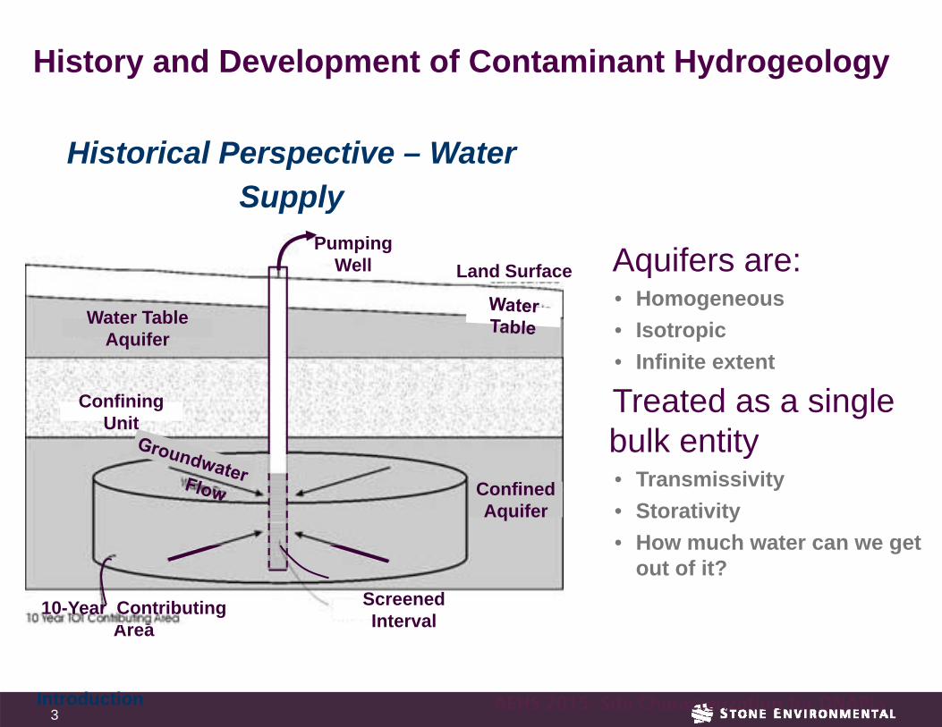
History and Development of Contaminant Hydrogeology
Historical Perspective – Water Supply
Aqquifers are: • Homogeneous • Isotropic •• Infinite extent Infinite extent
Treated as a single bulk entityy • Transmissivity • Storativity • How much water can we get How much water can we get
out of it?
Area
Pumping Well Land Surface Land Surface
Water Table Aquifer
Confining Unit
Confined Aquifer
10-Year Contributing Screened Interval
3 Introduction AEHS 2015: Site Characterization for DNAPLs

p p y pp p y y
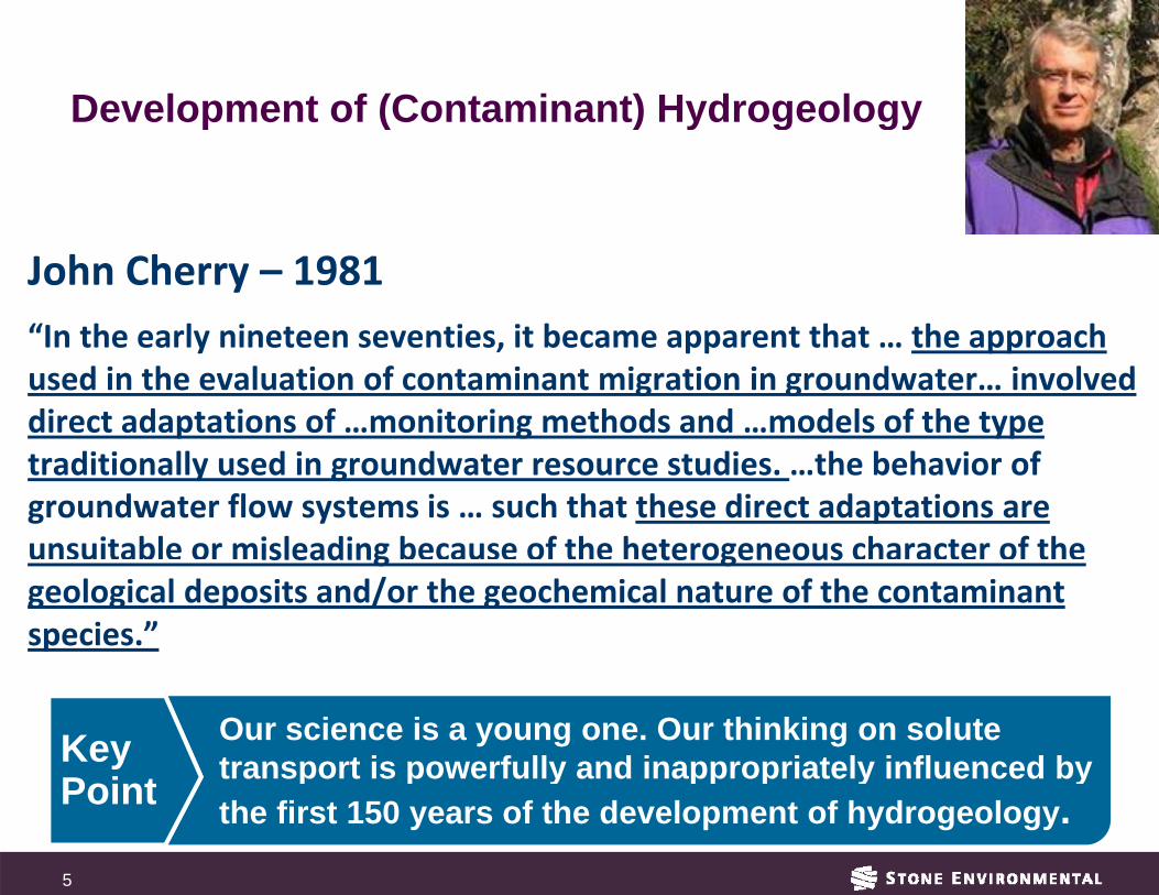
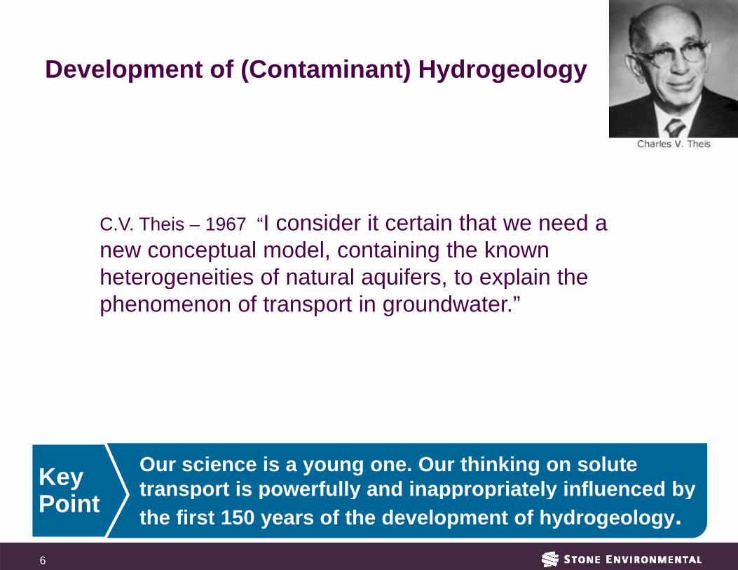
Development of (Contaminant) Hydrogeology Development of (Contaminant) Hydrogeology
~130-Year Era of Homogeneity and Isotropy
1970’s 1856 1870 1980 1986 2004
1863 1935 1979 1981 1994
Our science is a young one. Our thinking on solute transport is powerfully and inappropriately influenced byKey
Point the first 150 years of the development of hydrogeology. Point
4Introduction
unsuitable or m because of the h character of the
p p y pp p y y
Development of (Contaminant) HydrogeologyDevelopment of (Contaminant) Hydrogeology
John Cherry – 1981 “In the early nineteen seventies it became apparent that the approach In the early nineteen seventies, it became apparent that … the approach used in the evaluation of contaminant migration in groundwater… involved direct adaptations of …monitoring methods and …models of the type traditionally used in groundwater resource studies. …the behavior of groundwater flow systems is … such that these direct adaptations are unsuitable or misleading because of the heterogeneous character of theisleading eterogeneous geological deposits and/or the geochemical nature of the contaminant species.”
Our science is a young one. Our thinking on solute transport is powerfully and inappropriately influenced byKey
Point the first 150 years of the development of hydrogeology. Point
5
p p y pp p y y
Development of (Contaminant) HydrogeologyDevelopment of (Contaminant) Hydrogeology
C.V. Theis – 1967 “I consider it certain that we need a new conceptual model, containing the known heteroggeneities of natural aqquifers,, to expplain the phenomenon of transport in groundwater.”
Our science is a young one. Our thinking on solute transport is powerfully and inappropriately influenced byKey
Point the first 150 years of the development of hydrogeology. Point
6
-
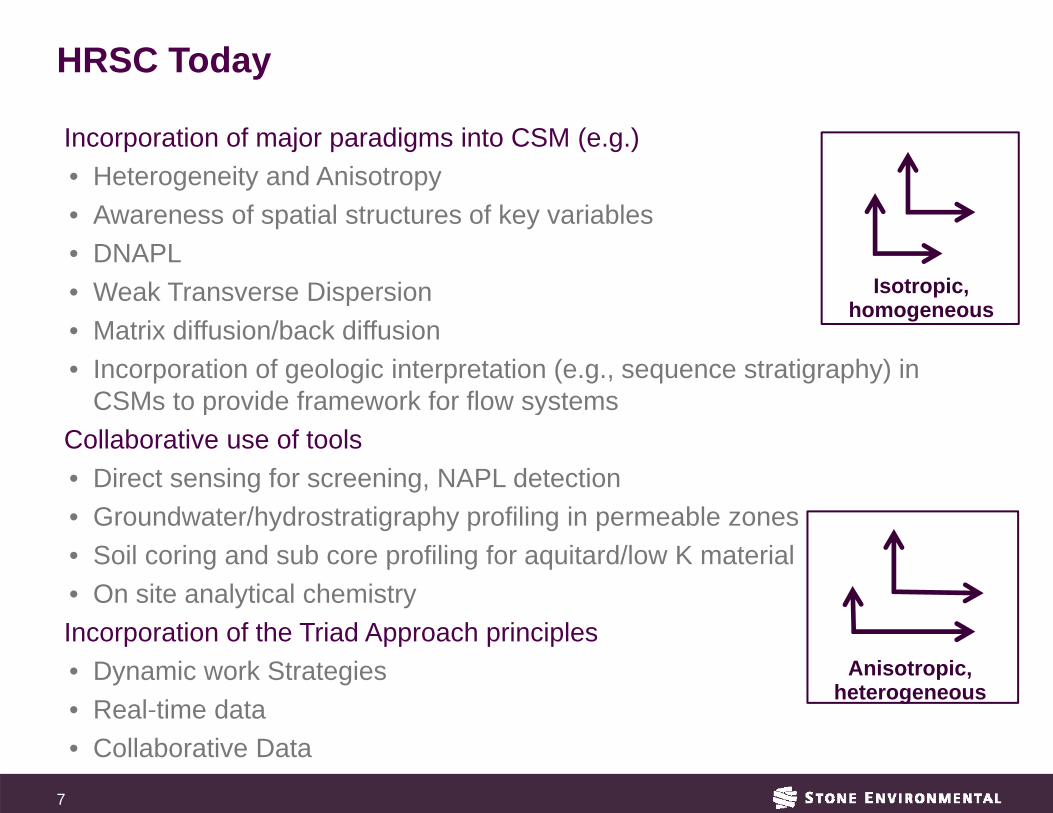
HRSC Today
Isotropic,h
Incorporation of major paradigms into CSM (e.g.) • Heterogeneity and Anisotropy • Awareness of spatial structures of key variables • DNAPL • Weak Transverse Disppersion • Matrix diffusion/back diffusion
homogeneous
• Incorporation of geologic interpretation (e.g., sequence stratigraphy) in CSMs to provide framework for flow systems CSMs to provide framework for flow systems
Collaborative use of tools • Direct sensing for screening, NAPL detection
G d t /h d t ti h fili i bl • Groundwater/hydrostratigraphy profiling in permeable zones • Soil coring and sub core profiling for aquitard/low K material • On site analytical chemistry Incorporation of the Triad Approach principles • Dynamic work Strategies •• Real-time data
Anisotropic,heterogeneous
Real time data • Collaborative Data
7

S li
HRSC Addresses Two Critical Issues
Sampling Scale and Data Averaging • Measurements must be made at a scale that is meaningful with respect to
the variability of the quantity being measured Coverage • Profiles and Transects • Horizontal spacing • Vertical spacing
SamplingScale and
Data Averaging
Coverage HRSC Data
8

Depth-Integrated, Flow Weighted Averaging El
evat
ionn
(m)
186 186
184 184
182182
180 180
178178 178178
176 176
1 10 100 1,000 10,000 100,000
10-3 10-2 10-1PCE (ug/L)
Hydraulic Conductivity(cm/sec) HydraulicConductivity(cm/sec)
9

High Resolution (more pixels): Sampling Scale and AveragingSampling Scale and Averaging
10
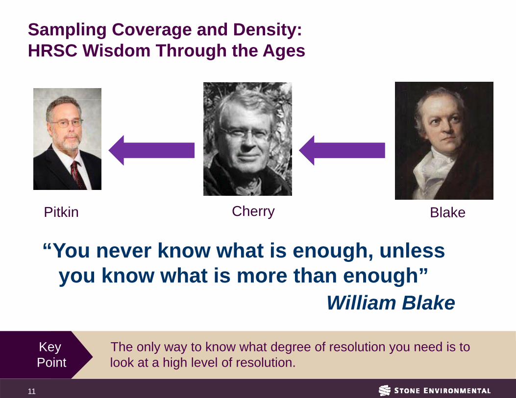
Sampling Coverage and Density: HRSC Wisdom Through the AgesHRSC Wisdom Through the Ages
Pitkin Cherry Blake
“You never know what is enough unlessYou never know what is enough, unless you know what is more than enough”
Willi BlWilliam Blakke
Key The only way to know what degree of resolution you need is to Key Point
The only way to know what degree of resolution you need is to look at a high level of resolution.
11
)D
epth
(
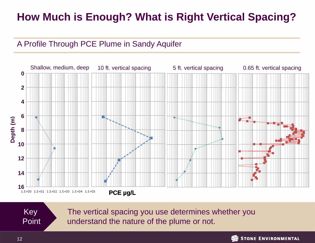
How Much is Enough? What is Right Vertical Spacing?
A Profile Through PCE Plume in Sandy Aquifer
5 ft. vertical spacingShallow, medium, deep
2
0
m
6
4
m
10
8
14
12
Key The vertical spacing you use determines whether you
16
Key Point
The vertical spacing you use determines whether you understand the nature of the plume or not.
10 ft. vertical spacing 0.65 ft. vertical spacing
PCE µg/LPCE µg/L
12

Multi-Level Sampling Transect PCE i PCE in a SSanddy AAquif ifer
Shallow, medium,
deepp
10 ft10-ft vertical spacing
0.8-ft vertical spacing
13What is HRSC? AEHS 2015 : Site Characterization for DNAPLs

mm-Scale Textural Changes Control DNAPL Migration
Poulsen & Kueper, 1992c
mc
m
~2
5~2
5
Key DNAPL distribution is controlled by capillary pressures that varyKey Point
DNAPL distribution is controlled by capillary pressures that vary at the mm scale. Distribution is very complex.
14

TCETCE DNAPLDNAPL
PlumePlume
Will the aquitardWill the aquitard DNAPLDNAPL the matrix pore waterthe matrix pore water
DNAPLs Commonly Encounter Aquitards
DissolvedDissolved massmass ininDissolvedDissolved massmass inin
stop the DNAPL?stop the DNAPL?( Mackay and Cherry, 1989 )
15

Double Wall, Sealable Joint Sheet Piling Cell Keyed into Aquitard
CFB Borden 9x9 m Cell CFB Borden 9x9 m Cell
Courtesy of Beth Parker
16

9 x 9 Meter Cell Experiment CFB Borden
770 Liters DNAPL PCE770 Liters DNAPL PCE Injected July 1991 DNAPL Distribution after 573 Hours
17

Borden 9x9 m Cell Experiment
DNAPL Injjection 1991
0Aquifer
3.3
6.0 Aquitard
9.0
Auger Holes 1991-94 9x9m Cell
0
DNAPL
Sand microbed zone
DNAPL
Sand microbed zone 11.5 Aquifer 13.5
HSA B HSA Boriing Outtside CCellllO id
Uh Oh!
Courtesy of Beth Parker
18

Areal Distribution of DNAPL within Aquitard
Section 3
DNAPL cell ZONE
DNAPL ONDNAPL ON TOP OF
AQUITARD
Section 2
Section 1
DNAPL
NO DNAPL
Section 2
0 10 m
Courtesy of Beth Parker
19

Structure and Pore Fluids Intact
Small Scale Features are of Great Import
DNAPL (red) migration Sand microbed in sand microbed
Courtesy of Beth Parker
20

Essential Information from Cores
Geologic/hydrogeologic features
Physical, chemical & microbial properties
Contaminant mass distributions (high- & low-K zones)
Contaminant phase distributions (detection of DNAPL)
Concentration gradients/diffusive fluxes
Effectiveness of remedial technologies
21

Soil Core Sampling - NAPL Detection
DNAPLStainless massSteel
Sampler Sorbed mass
Plunger
DissolvedDissolved mass
Sudan IV/OilSudan IV/Oil Red ORed OSample DDyyeeyyvollume
00 4 in4 inSoil coreSoil core Courtesy of Beth Parker
22

Methanol
Example of NAPL Detection
Sudan IV Screening Quantitative TCE Analyses
5 ft 10 ft TCE (ug/g wet soil) 0 100 200 300 400 500 600 700
00 Sudan IV positive
6’0”SudanIV test
) Methanol /L)
20
pth
(ft b
gs)
Extraction
y (1
200
mg/
30D
ep
E So
lubi
lity
Soil Core (SC5) TCE
positivep negative
10 6’1” 6’2”6 2
Sand Sand/siltSand
40
50
0 500 1000 1500 2000
Estimated Porewater TCE Estimated Porewater TCE Courtesy of Beth Parker (mg/L)
23

Groundwater Profiling - WaterlooAPS™ Integrated Data AcquisitionIntegrated Data Acquisition
• Physical Chemical Data
• Physical Chemical DataData
• Concentration Data• Hydraulic Head Data• Index of Hydraulic
Data • Concentration Data • Hydraulic Head Data • Index of Hydraulicy
Conductivity Datay
Conductivity Data
24

WaterlooAPS™ Configurations
Gas-Drive Pump Peristaltic Pump
Sample Line
Nitrogen Line
KPRO Line
KPRO + Sample Line
KPRO Line
1 ¾" Rod
1¾" Rod
Reed Valve
O-rings
¼" Stainless Steel Tubing
FEP Tubing
APS APS APS 225 175 150
25

WaterlooAPS™ Data Acquisition Configuration and ProcessConfiguration and Process
Notebook Data acquisition
electronics String potentiometer on drill computer
electronics rig/ Geoprobe® measures depth
Real-time Ik and Pressure
Reversible variable-speed peristaltic pump
or gas drive pump Water
Flow meter Real time Ik and
water quality data vacuum gauge or gas-drive pump quality sensor
Valve
Measures: Specificconductance pH
Pressure transducer
pH Dissolved O2 Oxidationreduction potential (ORP)
Compressed nitrogen
Stainless steel pressure vessel with analyte-free
water
1/8” stainless steel tubing
Sample bottles with stainless steel holders
Waterloo profiler tip with stainless steel screened inlet ports
26
Onsite lab

=
-50
Two Uses of IK Data
Sample Depth Selection Chlorobenzene (µg/L) Stratigraphic Interpretation
Upper
0
10ce)
Chlorobenzene (µg/L) 1 10 100 1000 10,000 100,000
Upper ClayUnit
-10
-20
ound
sur
fac
-30
, bel
ow g
ro
Elev
atio
n (f
e
-40
Dep
th (f
eet,
Stratigraphic Interpretation A A’
60
70
60
70
DPTSE27 DPTSE28
DPTSE30 DPTSE26
DPTSE23 DPTSE37 DPTSE21 DPTSE15
10
100 1,000 1,000
100
10,000 20
30
40
50
7J
2J
4J
730
5600
7J
200J
1050
2990
73200 77000
11770
9460
12360
650
<2<2ee
t)20
30
40
50
100 10
ND 100
-10
0
10
20
2J 2J
2J
<2
<2
2J
2J
<2 6J
5J
6J
8J
<2 4J
16
2J
14
200J
42 66
54
42
89
33 41 54 39
103 91 82
51
28
91
38 6260
41 54 56
79 131
12510 12360
48 34 <2
<2
<2
<2
<2
<2
-10
0
10
20
Aquitard
100
-40
-30
-20 2J 7J <2
120
33
<2 27
19
-40
-30
-20
Low Permeability Stratum
Isoconcentration (ug/L)
4900 Profiler Sample Location and Chemical Concentration (ug/L)
LEGEND
Note: MDL = 2 ug/L
100
-50-50 Note: MDL 2 ug/LD
IK Lower Aquitard Chlorobenzene-1-10000 00 100100 200200 300300 400400 500500 606000 770000 800800 900900 11000000 11001100 11200200 13001300 14014000
-60 0 2 4 6 8
IK – Index of Hydraulic Conductivity (unitless) K y y ( ) Horizontal Distance (feet)( )
27

Post-Remedy Investigation Northern England
Key Use of low resolution (conventional) techniques resulted in Key Point
Use of low resolution (conventional) techniques resulted in remedy failure and need for second remedy.
28
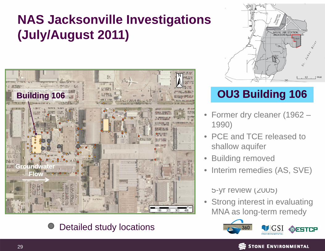
OU3 Building 106OU3 Building 106OU3 Building 106OU3 Building 106
have been discontinued after 5 review (2005)
NAS Jacksonville Investigations (J l /A t 2011)(July/August 2011)
OU3 Building 106OU3 Building 106Building 106Building 106 OU3 Building 106OU3 Building 106
• Former dry cleaner (1962 – 1990)
Building 106Building 106
1990) • PCE and TCE released to
shallow aquifer Building removed• Building removed
• Interim remedies (AS, SVE)
yr
GroundwaterGroundwater FlowFlow
5-yr review (2005) • Strong interest in evaluating
MNA as long-term remedy
Detailed study locations
29

NAS Jacksonville: Characterization Methods
Membrane Interface Probe (MIP) screening • Rappid lithology (EC) and contaminant ((ECD, PID)) delineation – qqualitativegy ( )
WaterlooAPS™ (Advanced Profiler System) •• Real time hydrostratigraphyReal-time hydrostratigraphy • Targeted groundwater sampling of higher K zones/interfaces
Geoprobe® HPT (Hydraulic Profiling Tool) • Real time hydrostratigraphy
Continuous cores (Geoprobe® DT System) • Detailed lithology delineation
Subsampling for mass distribution (targeted to lower K zones) • Subsampling for mass distribution (targeted to lower K zones)
Onsite Laboratory
30

- STONE ENVIRONMENTAL
Layout of Points at Each Investigation Location
31

NAS Jacksonville Composite Dataset (OU3(OU3-3 Near Source)3, Near Source)
gs)
?Dep
th (f
t bg
Mass in clay MIP Carry-Down in clayMIP Carry Down
Geoprobe®MIP WaterlooAPS™ Cores HPT
32

OU3-3: Soil and Groundwater Concentrations
543210
Index of Hydraulic Conductivity (Ik)
0 5 10 15 20 25 30
Soil CVOC Concentration (µg/kg)
0 5 10 15 20 25 30
Soil CVOC Concentration (µg/kg)
Soil Lithology
543210
2
0 0 5 10 15 20 25 30 0 5 10 15 20 25 30
NC
bgs)
2
4
SP
SP/CL
Dep
th (m
6 PCE Soil CL
SP/CL
8 Total CVOC Soil
Total CVOC GW (WP) PCE GW (WP)
cDCE GW (WP) TCE GW (WP)
cDCE Soil TCE Soil
SP
Groundwater CVOC
10 Total CVOC GW (Piezo/SP16)
0 30000 60000 90000 120000
cDCE GW (WP)
0 30000 60000 90000 120000
VC GW (WP)
Groundwater CVOCCVOC
Concentration CVOC
Concentration (µg/L) (µg/L)
33
-
Approximate boundaries of low K zone based on soil lithology
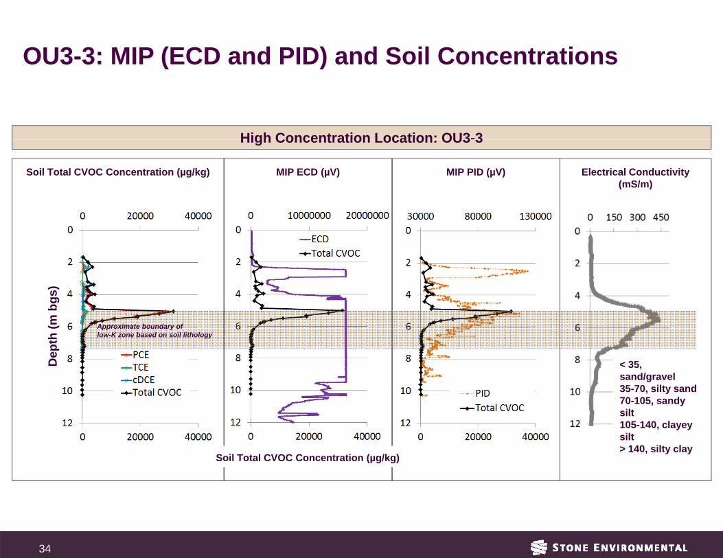
OU3-3: MIP (ECD and PID) and Soil Concentrations
High Concentration Location: OU3-3
Electrical Conductivity (mS/m)
High Concentration Location: OU3 3
MIP PID (µV) Soil Total CVOC Concentration (µg/kg) MIP ECD (µV)
Approximate boundary of low-K zone based on soil lithology
pth
(m b
gs)
< 35, sand/gravel 35-70, silty sand 70-105, sandy silt
Dep
105-140, clayey silt > 140, silty clay
Soil Total CVOC Concentration (µg/kg)
34

Collocated Soil Cores Demonstrate Good Correlation
Total Soil [VOC] (µg/g soil)
OC
sog
Tot
al C
VO
(µg/
g)
OU
3-5D
L
pth
(ft b
gs)
OU3-5 Log Total CVOCs (µg/g)
OC
s
Dep
og T
otal
CVO
(µ
g/g)
O
U3-
5D L
o
OU3-5 Log Total CVOCs (µg/g)
35

Dep
th (m
Sign
al (µ
V)
MIP Provides Mass Location But Not Concentration CorrelationConcentration Correlation
MIP: SOIL AT LOCATION OU3-3 MIP: SOIL AT LOCATION OU3-6 (HIGH CONCENTRATION)(HIGH CONCENTRATION) (LOW CONCENTRA(LOW CONCENTRATION) TION) USING OPTIMIZED SOP USING OPTIMIZED SOP
MIP ECD Signal (µV) MIP PID Signal (µV)
REGRESSIONREGRESSION
bgs)
Sign
al (µ
V)
Dep
th (m
bgs)
Log
PID
S
Log
ECD
S
Soil Total CVOC Concentration
Log PCE+TCE+DCE Soil Concentration (µg/kg)
Soil Total CVOC Concentration
Log PCE+TCE Soil Concentration
(µg/kg) (µg/kg) (µg/kg)
36

ee o eso ut o to u de sta d t e ob e t s s S te
Conclusion The purpose of Site Characterization is to understand the pertinent conditions adequately enough to devise an effective remedy. • aka CSM “Standard” approaches such as monitoring wells are not well suited to the development of such an adequate understanding • DepthDepth-integrated, flow weighted averagingintegrated, flow weighted averaging • Large life-cycle expense
S lScale off sampling and d d data coverage (d (densitit y)) must b t be appropriiatte tto theli t th spatial structure of the variable under consideration • Hydraulic conductivity, capillary pressure etc.
Leverage existing data and use screening technologies used to reduce costs associated with definitive sampling/analysis programs
Perhaps it is time to stop calling it “High Resolution” since it is really an adequate degree of resolution to understand the pproblem. It is simp y ply Siteadequate deg Characterization.
37

38
Acknowledgements
Beth Parker – University of Guelph Dave Adamson – GSIDave Adamson GSI Steven Chapman – University of Guelph Mike Singletary – NAVFAC


